Geosci. Model Dev., 5, 499–521, 2012 www.geosci-model-dev.net/5/499/2012/ doi:10.5194/gmd-5-499-2012 © Author(s) 2012. CC Attribution 3.0 License.
Geoscientific Model Development
A subgrid parameterization scheme for precipitation S. Turner, J.-L. Brenguier, and C. Lac Groupe d’Etude de l’Atmosph`ere M´et´eorologique/CNRM-GAME M´et´eo-France, URA1357, 42 Av Gaspard Coriolis, 31057 Toulouse Cedex 1, France Correspondence to: S. Turner (
[email protected]) Received: 19 April 2011 – Published in Geosci. Model Dev. Discuss.: 26 July 2011 Revised: 8 March 2012 – Accepted: 17 March 2012 – Published: 23 April 2012
Abstract. With increasing computing power, the horizontal resolution of numerical weather prediction (NWP) models is improving and today reaches 1 to 5 km. Nevertheless, clouds and precipitation formation are still subgrid scale processes for most cloud types, such as cumulus and stratocumulus. Subgrid scale parameterizations for water vapor condensation have been in use for many years and are based on a prescribed probability density function (PDF) of relative humidity spatial variability within the model grid box, thus providing a diagnosis of the cloud fraction. A similar scheme is developed and tested here. It is based on a prescribed PDF of cloud water variability and a threshold value of liquid water content for droplet collection to derive a rain fraction within the model grid. Precipitation of rainwater raises additional concerns relative to the overlap of cloud and rain fractions, however. The scheme is developed following an analysis of data collected during field campaigns in stratocumulus (DYCOMS-II) and fair weather cumulus (RICO) and tested in a 1-D framework against large eddy simulations of these observed cases. The new parameterization is then implemented in a 3-D NWP model with a horizontal resolution of 2.5 km to simulate real cases of precipitating cloud systems over France.
1
Introduction
In warm clouds, droplets form on activated cloud condensation nuclei (CCN) and grow by condensation of water vapor. Precipitation occurs when a few droplets grow large enough, typically within the range of 20 to 30 µm radius, for their sedimentation velocity to enhance the probability of collision and coalescence with smaller droplets. Observations have shown that such precipitation embryos are formed when the mean volume droplet radius of the droplet size distribu-
tion reaches a threshold of 10–12 µm (Gerber, 1996; Boers et al., 1998; Pawlowska and Brenguier, 2003). These embryos then become more efficient as they grow by collection, and precipitation develops until most of the cloud droplets have been collected (Pruppacher and Klett, 1997). The onset of precipitation is thus particularly sensitive to the likelihood of a few droplets (a few per liter) reaching this threshold radius. This depends on the local values of the liquid water content (qc ) and droplet number concentration (N ), as qc r = ( 4π 3ρ )1/3 . The key issue here is that the onset of pre/ wN cipitation is a small-scale process, typically on the scale of a convective cell core, i.e. a few tens of meters. This process is well reproduced with Large Eddy Simulations (LES) and bulk microphysics schemes (Khairoutdinov and Kogan, 2000; Stevens et al., 1996; Morrison and Grabowski, 2008), but coarser resolution Numerical Weather Prediction models (NWP) and climate models have difficulties simulating precipitation formation because clouds occupy only a fraction of the grid and the grid mean values of the bulk microphysical parameters are not representative of the peak values occurring at a few local spots. Long-term observations of clouds and precipitation made within the framework of the Cloudnet project show that the UK Unified model captures the frequency of occurrence of clouds and precipitation, and the diurnal cycle in cloud height reasonably well, on average (Illingworth et al., 2007; Barrett et al., 2009), but two major shortcomings of the model have also been identified. First, the model underestimates the frequency of occurrence of overcast grid boxes by a factor of two; second, values of drizzle rate greater than 0.1 mm h−1 are ten times more frequent in the model than in the observations. Such biases are also observed with the ECMWF and ALADIN models, which show a clear overestimation in light precipitation. The impact is not as strong for surface precipitation since most drizzle evaporates before reaching the ground, but rather for the overall dynamics of the boundary
Published by Copernicus Publications on behalf of the European Geosciences Union.
500
S. Turner et al.: A subgrid parameterization scheme for precipitation
layer because of the resulting enhanced cooling of the subcloud layer, which leads to clouds dissipating too rapidly. When cloud properties are statistically homogeneous within a model grid (≥50 km), empirical relationships can be derived between precipitation rate at cloud base, cloud liquid water path (LWP) and the mean value of the concentration of activated nuclei (Nact ). Such relationships were initially derived from field experiments such as ACE-2 (Pawlowska and Brenguier, 2003), EPIC (Comstock et al., 2004) and DYCOMS-II (van Zanten et al., 2005), and they have been further corroborated by LES simulations of stratocumulus (Geoffroy et al., 2008) and cumulus fields (Jiang et al., 2010). At higher horizontal resolutions, however, only few clouds occupy the model grid, and such a statistical approach is no longer valid. The issue is analogous to the simulation of water vapor condensation, which called for the implementation of subgrid cloud schemes (Sommeria and Deardorf, 1977): the relative humidity fluctuations in a model grid are represented by a Probability Density Function (PDF) specified a priori and the fraction of the PDF with humidity values greater than 100 % determines the cloud fraction (CF). With such an artifice, the transition from clear to fully cloudy grids is smoothed out and the non-linear interactions (radiation for instance) are better represented. For radiative transfer calculations, however, additional hypotheses are necessary to vertically overlap the cloud fractions diagnosed independently at each model level. Similarly, subgrid rain schemes aim at simulating the gradual transition from non-precipitating to fully precipitating model grids. Because of the non-linearity of the onset of precipitation, such a scheme is expected to significantly impact simulations of shallow convective clouds in which the grid mean values of the droplet mean volume diameter hardly reach the collection threshold while local values might. Subgrid schemes thus attempt to calculate the grid mean impact of non-linear physical processes when the grid mean values of the state parameters are specified. In a statistical approach, the key issue is therefore to select universal distributions to represent the subgrid variability of the atmospheric state parameters. The challenge is that such distributions are not statistically independent since many cloud processes depend on their joint variability. For instance, depends jointly on temperature and humidity through relative humidity, but more precisely on their joint variability, which determines the probability of the relative humidity reaching 100 % in a model grid. Parameterization of precipitation introduces an additional level of complexity since the rate of droplet accretion by drops depends on the product of the cloud and precipitating water mixing ratios. A few alternative approaches have therefore been explored to get around this problem, in which the equations are allowed to build the convective structures but in a simplified two-dimensional framework. These approaches are referred to as superparameterization (Grabowski, 1999), quasiGeosci. Model Dev., 5, 499–521, 2012
3-D Multi-scale Modeling Framework (Arakawa, 2004), or Macro-Micro-Interlocked algorithm (Kusano et al., 2007). Within the framework of the statistical approach, new techniques have also been developed to stochastically sample the possible states of the system with the purpose of decreasing the cost of the parameterization without reducing its level of complexity. They include the Joint PDF approach of Golaz et al. (2002), the generation of a cloudy sub-column with Full Generator (FGen) by R¨ais¨anen et al. (2004), precipitation formation using the Latin Hypercube Sampling by Larson et al. (2005), the cellular automatons of Berner (2005), and the stochastic activation of convection by Tompkins (2005). The scheme tested here is based on the PDF approach introduced by Sommeria and Deardorff (1977), which has been extensively used for subgrid condensation (Bougeault, 1981; Tompkins, 2002; Bony and Emanuel, 2001). The onset of precipitation still relies on the mean cloud fraction value of the cloud water content while, locally, peak values can reach the collection threshold and initiate precipitation before the mean value is reached. Following Bechtold et al. (1993), the variability of the cloud water content in the cloud fraction of a model grid is represented by a PDF and precipitation is initiated in the subcloud fraction where the values of the cloud water content are greater than the collection threshold. This cloud water splitting for rain formation is similar to the Tripleclouds scheme developed for radiation purposes by Shonk and Hogan (2008), although the splitting is not arbitrarily specified here but depends rather on the comparison with the threshold radius for collection. The modeling context is described in the following section with more details on the bulk microphysics scheme. After a presentation of the subgrid parameterization of precipitation in Sect. 3, two boundary layer cases of stratocumulus and cumulus clouds will be used to compare observations with LES and SCM (single column model) simulations in Sects. 4 and 5, respectively. The results obtained with the research model for a real (3-D) case of precipitating boundary layer clouds are presented in Sect. 6, followed by our conclusions.
2
Modeling context and methodology
The horizontal resolution of most of current state-of-the-art operational mesoscale forecast models now reaches 1–5 km, which allows to explicitly resolve cloud structures. In NWP mesoscale models, single moment bulk microphysics parameterizations are currently used for precipitation processes, with mixing ratios of the different species as prognostic variables. If the impacts of aerosols on clouds (aerosol indirect effects) are to be accounted for, double moment schemes have to be used, with additional variables for the number concentrations of cloud and precipitation particles. This study was done to improve small-scale precipitations for M´et´eo-France NWP model AROME (2.5 km, Seity et al., 2011). The parameterizations of the physical processes are www.geosci-model-dev.net/5/499/2012/
S. Turner et al.: A subgrid parameterization scheme for precipitation derived from those developed for the non-hydrostatic anelastic research model Meso-NH (Lafore et al., 1998), while the dynamical core comes from the regional ALADIN nonhydrostatic operational model (Bubnova et al., 1995). The AROME and Meso-NH models use a statistical subgrid condensation scheme to diagnose the cloud fraction using subgrid scale cloud variability from the turbulence (Bougeault, 1982; Bechtold et al., 1995) and the shallow convection scheme (Pergaud et al., 2009). Both models use the ICE3 single moment microphysical scheme (Pinty and Jabouille, 1998). The subgrid precipitation scheme is tested in this framework, but limited to warm precipitation, although it can be extended to mixed microphysics and adapted to double moment schemes. The development of a PDF-type subgrid scheme raises two issues: first the selection of a universal function for the PDF that realistically reflects statistical distribution of the small scale microphysical parameter values and, second, the definition of rules for the vertical overlap of the subgrid fractions, cloudy and clear air fractions and, inside the cloudy fraction, the precipitating and non-precipitating fractions. The first issue is addressed by analyzing airborne data collected in shallow convective clouds, stratocumulus (DYCOMS-II) and cumulus (RICO). Airborne data, however, covers a very limited fraction of the domain. To extend the 3-dimensional characterization of the microphysical fields, LES are performed with the Meso-NH model. After validation of the simulations against the observations, the simulated fields are used to complement the statistics. 2.1
The Meso-NH LES simulations
The DYCOMS-II and RICO cases were run using the LES version of Meso-NH with a timestep of 1 s and fine horizontal and vertical resolutions (see Table 1). The turbulent scheme was a 3-D turbulent kinetic energy (TKE) scheme (Cuxart et al., 2000) with a Deardorff mixing length. PBL clouds were assumed to be resolved at the LES resolution with “all or nothing” condensation. Microphysical schemes were either the one-moment scheme of Pinty and Jabouille (1998), also referred to as the ICE3 or SM (Single Moment) scheme, or the two-moment scheme of Cohard and Pinty (2000), referred to as the C2R2 scheme, or the scheme by Geoffroy et al. (2008), also referred to as the KHKO scheme (both twomoment schemes will be further referenced as DM, Double Moment). The DM scheme rely on four prognostic variables: the cloud droplet and drizzle/rain drop concentration, and the cloud droplet and drizzle/rain drop mixing ratios. A fifth prognostic variable is used to account for already activated CCN, following the activation scheme of Cohard et al. (1998), which is an extension of the Twomey (1959) parameterization for more realistic activation spectra. The number of CCN, activated at any time step, is equal to the difference between the number of CCN which would activate at the diagnosed pseudo-equilibrium peak supersaturation in www.geosci-model-dev.net/5/499/2012/
501
the grid (depending on updraft velocity and temperature) and the concentration of already activated aerosols. DM simulations were performed here with activation spectra producing concentrations of activated nuclei at 1 % supersaturation of 50, 70, and 100 cm−3 , called DM-50, DM-70 and DM-100, respectively. 2.2
The Meso-NH SCM simulations
In order to test the new parameterization for operational mesoscale models (1–5 km), the Meso-NH model was also used in a single column (SCM) mode initialized with the same forcing fields as for the DYCOMS-II and RICO LES. Table 1 shows some differences between LES and SCM simulations. The SM scheme was used in all SCM simulations, without (SM-CTRL) or with (SM-NEW) the new subgrid rain parameterization. 3
Subgrid rain parameterization scheme
The Meso-NH model already uses a subgrid scheme for cloud fraction (CF). Note, however, that the new scheme will also work without a cloud fraction scheme (CF = 1), although the potential benefits would probably be limited in such cases. 3.1
Splitting of the cloud water PDF
We defined the local value of the cloud water content (CWC) in the cloudy fraction as q˜c = q¯c /CF, where q¯c is the grid mean value in the model. In the cloud fraction, the CWC PDF was represented by an analytical function (f(q˜c )) with one parameter that was constrained by its first moment, q˜c . The cloudy fraction was then divided into two parts, in which the local values of the cloud water mixing ratio were respectively lower (CFL ) and higher (CFH ) than the autoconversion threshold of the microphysical scheme (see Appendix A for the values of the autoconversion scheme used in this study). The CWC mean values in the CFL and CFH subcloud fractions are defined as for the first moment of the PDF, were q˜cL is integrated from 0 to the collection threshold qcR , which can be of Kessler type or any other one, and q˜cH is the integration of all values higher than qcR . The grid mean values were similarly split in two parts: CF = CFH + CFL
(1)
q¯c = q¯cH + q¯cL
(2)
By definition, there is no production of precipitating particles in CFL and the autoconversion scheme (Kessler, 1969) was only applied in CFH with a CWC value equal to q˜cH . 3.2
The cloud water PDF
Statistics of cumulus CWC derived from past observations and LES cases suggest that linear or quadratic decreasing Geosci. Model Dev., 5, 499–521, 2012
502
S. Turner et al.: A subgrid parameterization scheme for precipitation
Table 1. Set-up for LES and SCM simulations of DYCOMS-II and RICO.
Horizontal resolution Number of grid points Horizontal domain Vertical resolution Number of levels Domain height Timestep Total duration
DYCOMS-II Simulations LES (3-D) SCM (1-D)
RICO Simulations LES (3-D) SCM (1-D)
50 m 128 × 128 6.4 km
2.5 km 1×1 –
100 m 128 × 128 12.8 km
2.5 km 1×1 –
10 m 150 1.5 km
10 m 150 1.5 km
40 m 100 4 km
40 m 100 4 km
1s 6h
10 s 6h
1s 24 h
10 s 24 h
Table 2. Maximum values of CWC (qcM ) and local mean values of CWC in low (e qcL ) and high (e qcH ) CWC regions for four different CWC PDF forms. The threshold value allowing precipitation formation is identified with qcR . Distribution forms
qcM
e qcL
e qcH
rectangular
2e qc
rectangular triangular
3e qc
quadratic
4e qc
qcR 2 2 3qcM qcR − 2qcR 6qcM − 3qcR 3 − 8q 2 q 2 3qcR cR cM + 6qcR qcM
qcM + qcR 2 qcM + 2qcR 3 qcM + 3qcR
2e qc
2 − 12q q 2 4qcR cR cM + 12qcM 3 3 2 qcM − 12qcM qcR + 8qcR
4 qcM + 2qcR
2e qc
2 − 24q q + 12q 2 6qcM cM cR cR 2qcR
3 3 − 8q 3 3qcM cR
3
2 − 12q 2 6qcM cR
isosceles triangular (e qc ≤ qcR ) isosceles triangular (e qc > qcR )
functions could be suitable for describing its PDF (as it will be shown later in Fig. 12). To evaluate the sensitivity of the scheme to the PDF choice, tests were extended to rectangular and two triangular PDF, as shown by Fig. 1. A variable named qcM was added as the limit for the integration of the CWC and it is derived from the conservation of the CWC in the grid box. Figure 1 shows all four PDF with the low (light grey) and high (dark grey) CWC regions for q˜c < qcR (left column) and q˜c > qcR (right column). Table 2 shows how parameters of the distribution were derived from the mean CWC value in the cloud fraction. Figure 2 shows how qcM , q˜cL and q˜cH increased with increasing values of q˜c . In fact, the different PDF shapes did not significantly affect the relationship between the mean CWC value in the cloud fraction and the mean of the values higher than the collection threshold that drove the autoconversion rate. As soon as the CWC is split into a high and a low part, q˜cH > q˜c , but there is little difference between the q˜cH values derived using the four different PDF forms.
Geosci. Model Dev., 5, 499–521, 2012
3.3
Rain fraction
The local value of rain water content (RWC) was defined, like the local value of cloud water, as q˜r = q¯r /RF, where RF is the rain fraction in the model grid. The rain fraction, however, could not be diagnosed like the cloud fraction because rain drops fall to the ground. The challenge was to address this probabilistic issue without adding more prognostic variables into the model. When precipitation forms in a model grid void of precipitating drops, the solution is straightforward since it is confined to the grid fraction where q˜cH becomes greater than the collection threshold and RF is initially set to CFH . A realistic approach would be to advect the rain fraction like any conservative variable, considering that the fraction is uniformly distributed over each model grid. This is feasible if one more prognostic variable is added, namely the subgrid value of the RWC. After advection, the rain fraction can thus be calculated as q˜r /q¯r . At this stage, however, a simpler, economical solution was tested that did not require an additional variable. The RWC is advected like all other model variables and the rain fraction is following the rain in the column: once precipitation had formed in a model column, www.geosci-model-dev.net/5/499/2012/
S. Turner et al.: A subgrid parameterization scheme for precipitation
503
q�c < qcR a1
Rectangular PDF
q�c > qcR a2
b1
Rectangular triangular PDF
b2
c1
d1
Quadratic PDF
Isosceles triangular PDF
c2
d2
Figure 1: four Graphs theused fourtoPDF forms represent the CWC. Light represents of Fig. 1. Graphs of the PDF of forms represent theused CWC.toLight grey represents regions of grey low CWC and darkregions grey represents high e CWC. Thelow localCWC meanand CWC, thegrey localrepresents low CWC and highThe CWC are, mean respectively, qthe qcL andlow qcH .CWC The autoconversion dark highlocal CWC. local CWC,e local and local highthreshold is c, e qcR , and the maximum value of the CWC CWC are, respectively, q�c , q�iscLqand �cH . The autoconversion threshold is qcR , and the maximum value of cM . q the CWC is qcM .
the rain fraction was translated to the whole column below, the rain fraction to zero in grids where the RWC was less down to the ground. In other words, the rain fraction in a than a small threshold value. model column was equal to the maximum of the rain frac3.4 Vertical overlap tions at the levels where rain is formed. Note that there is Vertical overlap of clouds and rain fractional areas is also a no horizontal advection of the rain fraction. Because RWC probabilistic issue. In order to maximize precipitation forcan be advected but its fractional part cannot, possible inconsistencies between this simple probabilistic approach and the 25 mation for cumulus and stratocumulus clouds, the maximum cloud overlap assumption was used for CF and RF in the new 3-D advection of RWC were further accounted for by setting parameterization (see Fig. 3). www.geosci-model-dev.net/5/499/2012/
Geosci. Model Dev., 5, 499–521, 2012
504
S. Turner et al.: A subgrid parameterization scheme for precipitation
a) qcM
b) q�cL (solid) and q�cH (dotted)
c) CFL /CF (solid) and CFH /CF (dotted)
Fig. 2. Variations of (a) the CWC (qcM ), (b) the (q mean local qcL , solidlocal lines) low and high , dotted lines)and CWC and Figure 2: Variations ofmaximum (a) the maximum CWC (b)low the(e mean (� qcL(e ,qcH solid lines) high cM ), (c) the relative cloud fractions in low CWC region (solid lines) and high regions (dotted lines) as a function of e qc . The four PDF forms are (� qcH , dotted lines) CWC and (c) the relative cloud fractions in low CWC region (solid lines) and high rectangular (blue), rectangular triangular (red), quadratic (green) and isosceles triangular (pink). A vertical dashed grey line is added at the regions (dotted lines) asthat a function of q�c . lines Thearefour rectangular (blue), rectangular autoconversion threshold. Note two grey reference addedPDF in (b)forms and (c), are and the blue line is overlapping the pink one intrian(a) . gular (red), quadratic (green) and isosceles triangular (pink). A vertical dashed grey line is added at the autoconversion threshold. Note that two grey reference lines are added in Fig. b and c, and the blue line Following the same concept, it was assumed that the rain fell through clear air. Such an assumption mimics the LES is overlapping thepreferentially pink one ininFig. fraction sedimented the a. cloud core (CFH ). when clouds are growing vertically, but it obviously fails for
If RF> CFH , the remainder rainwater fell from the diluted cloud fraction CFL and if RF>CF, the remaining rainwater
Geosci. Model Dev., 5, 499–521, 2012
multi-layered clouds or when clouds are tilted because of wind shear.
www.geosci-model-dev.net/5/499/2012/
S. Turner et al.: A subgrid parameterization scheme for precipitation
505
Table 3. List of C-130 flights for DYCOMS-II used in this study. Drizzle rates are from van Zanten et al. (2005). Flight number
Date
RF01 RF02 RF03 RF04 RF05 RF07 RF08
20010710 20010711 20010713 20010717 20010718 20010724 20010725
Flight condition
Drizzle rate (mm day−1 )
night night night night night night day
none 0.35 ± 0.11 0.05 ± 0.03 0.08 ± 0.06 none 0.60 ± 0.18 0.12 ± 0.03
Fig. 3. The three columns are the successive steps of the numerical ure 3: The three columns are cloud the successive steps ofoverlap the numerical treatment treatment of the and rain vertical in a model columnof the cloud and rain ical overlap in a model column. (a) The maximum cloud overlap is applied with 5 levels: k1, k2, k3, k4, and k5. (a) The maximum cloud over- for adjacent or nona. RF = CFH : accretion is calculated using q˜cH and there acent layers. lap (b) is The same for maximum overlap of (A) is applied for same the new parameterization applied adjacentcloud or non-adjacent layers. (b) The is no evaporation (see Fig. 4a). ng the splittingmaximum of the CWC in two regions, and maximally overlapping the high CWC regions. (c) The cloud overlap of (a) is applied for the new parameterizais falling vertically with a maximum vertical overlap. tion using the splitting of the CWC in two regions, and maximally overlapping the high CWC regions. (c) The rain is falling vertically with a maximum vertical overlap.
b. CFH