ing hypergraph matching problem is formulated as the max- imization of a
multilinear ..... This method does not reach a global optimum. However, it
converges to ...
A Tensor-Based Algorithm for High-Order Graph Matching Olivier Duchenne1,4 1
Francis Bach1,2,4
´ Willow / Ecole Normale Sup´erieure de Paris1
Inso Kweon3 2
{duchenne,bach,ponce}@ens.fr
Abstract This paper addresses the problem of establishing correspondences between two sets of visual features using higher-order constraints instead of the unary or pairwise ones used in classical methods. Concretely, the corresponding hypergraph matching problem is formulated as the maximization of a multilinear objective function over all permutations of the features. This function is defined by a tensor representing the affinity between feature tuples. It is maximized using a generalization of spectral techniques where a relaxed problem is first solved by a multi-dimensional power method, and the solution is then projected onto the closest assignment matrix. The proposed approach has been implemented, and it is compared to state-of-the-art algorithms on both synthetic and real data.
1. Introduction Establishing correspondences between two sets of visual features is a key problem in computer vision tasks as diverse as feature tracking [5], image classification [15] or retrieval [23], object detection [4], shape matching [28, 16], or wide-baseline stereo fusion [21]. Different image cues may lead to very different matching strategies. At one end of the spectrum, geometric matching techniques such as RANSAC [8], interpretation trees [11], or alignment [12] can be used to efficiently explore consistent correspondence hypotheses when the mapping between image features is assumed to have some parametric form (e.g., a planar affine transformation), or obey some parametric constraints (e.g., epipolar ones). At the other end of the spectrum, visual appearance alone can be used to find matching features when such an assumption does not hold: For example, bagsof-features methods that discard all spatial information to build some invariance to intra-class variations and viewpoint changes have been applied quite successfully in image classification tasks [26, 27]. Modern methods for image 4 WILLOW project-team, Laboratoire d’Informatique de l’Ecole Normale Sup´erieure, ENS/INRIA/CNRS UMR 8548.
INRIA
Jean Ponce1,4 3
KAIST
[email protected]
matching now tend to mix both geometric and appearance cues to guide the search for correspondences (see, for example, [15, 18]). Many matching algorithms proposed in the 80s and 90s have an iterative form but are not explicitly aimed as optimizing a well-defined objective function (this is the case for RANSAC and alignment methods for example). The situation has changed in the past few years, with the advent of combinatorial or mixed continuous/combinatorial optimization approaches to feature matching (see, for example [4, 19, 20, 28, 16]).1 This paper builds on this work in a framework that can accommodate both (mostly local) geometric invariants and image descriptors. Concretely, the search for correspondences is cast as a hypergraph matching problem using higher-order constraints instead of the unary or pairwise ones used by previous methods: Firstorder methods based (for example) on local image descriptions are susceptible to image ambiguities due to repeated patterns, textures or non-discriminative local appearance for example. Geometric consistency is normally enforced using pairwise relationships between image features. In contrast, we propose in this paper to use higher-order (mostly thirdorder) constraints to enforce feature matching consistency (see Figure 1) This work generalizes the spectral matching method of [16] to higher-order potentials: The corresponding hypergraph matching problem is formulated as the maximization of a multilinear objective function over all permutations of the features. This function is defined by a tensor representing the affinity between feature tuples. It is maximized by first using a multi-dimensional power method to solve a relaxed version of the problem, whose solution is then projected onto the closest assignment matrix. The three main contributions are (1) the application of the tensor power iteration for the high-order matching task, used with a tighter relaxation based on constraints on the column norms of assignment matrices, (2) the design of appropriate similarity measures which can be chosen ei1 To
be fair, it should be noted that optimization-based approaches to graph matching were considered a key component of object recognition and scene analysis strategies in the 70s, see for example the classical text by Ballard and Brown [3, Ch. 11].
Figure 1. Left: second-order potentials can be rotation-invariant by comparing distances between matched points. Right: Thirdorder potentials can be similarity-invariant by comparing angles of triangles.
ther to improve invariance of the matching, or to improve the expressivity of the model (see Section 5), and (3) an `1 -norm relaxation instead of the classical `2 -norm relaxation, that allows solutions which are more discriminative but still allows efficient power iteration solutions (see Section 4). The proposed approach has been implemented, and it is compared to state-of-the-art algorithms on both synthetic and real data. As shown by our experiments (Section 7), our implementation is, overall, as fast as these methods in spite of the higher complexity of the underlying model, with better accuracy on standard databases. The source code of our software is available online at http: //www.di.ens.fr/˜duchenne.
2. Graph matching for computer vision 2.1. Previous work As noted earlier, finding correspondences between visual features (such as interest points, edges, or even raw pixels) is a key problem in many computer vision tasks. The simplest approach to this problem is to define some measure of similarity between two features (e.g., the Euclidean distance between Sift descriptors of small image patches [18]), and match each feature in the first image to its nearest neighbor in the second one. This naive approach will fail in the presence of ambiguities such as repeated patterns, textures or non-discriminative local appearance. To handle this difficulty, some papers try to enforce some geometric consistency between pairs of feature correspondences. The basic idea is that if the points p1 and p01 of image 1 are matched to points p2 and p02 of image 2, then the geometric relation between p1 and p01 , and the ones between p2 and p02 should be similar. Several pairwise geometric relations have been used. Leordanu and Hebert [16] use only the distance between two points, leading to a potential which is invariant to rotation. Berg et al. [4] use a combination of potential based on distance and based on angle (scale invariant), to find a trade-off between rotation and scale invariance. Some other methods (e.g., [23, 28]) use neighborhoods, by only assuming that neighbor points should be matched to neigh-
bor points. One difficulty here is to define an appropriate notion of neighborhood. Recently, the computer vision community has put much effort in increasing the order of complexity of the models used: For example, Kohli et al. [13] introduce a highorder clique potential for segmentation, but the type of energy is limited to specific types of functions, and the alpha-expansion framework used there leads to a local optimum. Moreover, Zass and Sashua [25] formulate the search for higher-order feature correspondences as a hypergraph matching problem. We will use the same formulation but a different optimization setup. In addition, unlike these authors, we will refrain from using independence assumptions (that may or may not be justified depending on the situation) to factor our model into first-order interactions. As will be shown in the comparative experiments of Section 7, explicitly maintaining higher-order interactions in the optimization process will lead to superior performance.
2.2. Mathematical Formulation We consider two images, and assume that we have extracted N1 features from image 1, and N2 features from image 2. We do not assume that N1 = N2 , i.e., there may be different numbers of points in the two images to be matched. Throughout this paper, for s = 1, 2, all indices is , js , ks will be assumed to vary from 1 to Ns . We will also note i = (i1 , i2 ), j = (j1 , j2 ), k = (k1 , k2 ) pairs of potentially matched points. Let Pis be the ith point of image s. The problem of matching points from image 1 to points from image 2 is equivalent to looking for an N1 × N2 assignment matrix X such that Xi1 ,i2 is equal to 1 when Pi11 is matched to Pi22 , and to 0 otherwise. In this paper, we assume that a point in the first image is matched to exactly one point in the second image, but that two points in the second image may be matched to an arbitrary number of points in the first image, i.e., we assume that the sums of each column is equal to one, but put no with constraints on the row sums. (this framework can easily be extended to allow matching points from the first image to no points in the second image using dummy nodes such as in[4]). Thus, we consider the set A of assignment matrices: A = {X ∈ {0, 1}N1 ×N2 ,
P
i1
Xi1 ,i2 = 1}.
Note that our definition is not symmetric (i.e., if we switch the two images, we obtain different matchings). It can simply be made symmetric by considering the two possible matchings and combining them in a (mostly applicationdependent way), e.g., by taking the union or intersection of matchings. In [4, 7, 16], the matching problem is formulated as the
maximization of the following score on A:
score(X) =
X
needed for matching.
Hi1 ,i2 ,j1 ,j2 Xi1 ,i2 Xj1 ,j2 ,
i1 ,i2 ,j1 ,j2
where Hi1 ,i2 ,j1 ,j2 (which is equal to Hi,j with our notations for pairs) is a binary potential corresponding to the pairs of points (Pi1 , Pj1 ) of image 1, and (Pi2 , Pj2 ) of image 2. High values of H correspond to similar pairs. This graph matching problem is actually an integer quadratic programming problem, with no known polynomial-time algorithm. Approximate methods may be divided into two groups of algorithms. The first group is composed of methods which use spectral representations of adjacency matrices (see, e.g., [24, 16]). The second group is composed of algorithms which work directly with graph adjacency matrices, and typically involve a relaxation of the complex discrete optimization problem (see, e.g., [2]). In this paper, we focus on improvements on spectral methods. In [7, 16], the set of matrices over which the optimization is performed is thus relaxed to the set of matrices with 1/2 Frobenius norm kXkF equal to N2 , leading to the simpler problem:
max
X
1/2 kXkF =N2 i ,i ,j ,j 1 2 1 2
Hi1 ,i2 ,j1 ,j2 Xi1 ,i2 Xj1 ,j2 .
(1)
In turn, this can be rewritten as maxkXkF =N 1/2 X T HX 2 where, abusing the notation, X is this time considered as a N1 N2 vector, and H as an N1 N2 by N1 N2 symmetric matrix. This is a classical Rayleigh quotient problem, whose 1/2 solution is N2 times the eigenvector X ∗ associated with the largest eigenvalue (which we refer to as the main eigenvalue) of the matrix X [9], and can be computed efficiently by the power iteration method described in the next section. An important constraint that is put on H is that it is pointwise non-negative. In this situation, the Perron-Frobenius theorem [9] ensures that X ∗ only has non-negative coefficients, which simplifies the interpretation of the result: In order to obtain an assignment matrix in A, i.e., a matrix with elements in {0, 1} and proper column sums, the matching is discretized using a greedy algorithm.
2.3. Power iteration for eigenvalue problem The power iteration method is a very simple algorithm for computing the main eigenvector of a matrix, which is
Input: matrix H Output: V main eigenvector of H 1 initialize V randomly ; 2 repeat 3 V ← HV ; 4 V ← V /kV k2 ; 5 until convergence ; Algorithm 1: Power iteration for eigenvalue problem. This algorithm converges geometrically to the largest eigenvalue of the input matrix [9]. In our situation, H is very sparse and we want to take advantage of it. Each step of the power iteration algorithm requires only O(m) operations, where m is the number of non-zero elements of H. Typically, in our situations, the algorithm converges in around 20 steps.
3. Tensor formulation We propose to use tensors to solve the high-order feature matching problem. Indeed, using tensors is quite natural to generalize the idea of spectral matching [16] which deals with a matrix. Previous works only use point-to-point and pair-to-pair comparisons for their matching. In this paper, we want to compare tuples of points. So, we now want to add higher-order terms to the score function defined in Eq. (1). For simplicity, we will focus from now on thirdorder interactions. Generalizations to higher-order potentials is (in theory at least) straightforward. We define a new high-order score: X score(X) = Hi1 ,i2 ,j1 ,j2 ,k1 ,k2 Xi1 ,i2 Xj1 ,j2 Xk1 ,k2 , (2) i1 ,i2 ,j1 ,j2 ,k1 ,k2
where we assume that we have a super-symmetric tensor, i.e., invariant by permutation of indices in {i1 , j1 , k1 } or {i2 , j2 , k2 }. Here, the product Xi1 ,i2 Xj1 ,j2 Xk1 ,k2 will be equal to 1 if the points {i1 , j1 , k1 } are all matched to the points {i2 , j2 , k2 }, and 0 otherwise. In the first case, it will add Hi1 ,i2 ,j1 ,j2 ,k1 ,k2 to the total score function. This is a similarity measure, which will be high if the sets of features {i1 , j1 , k1 } is similar to the set {i2 , j2 , k2 }. Note that we can rewrite the score compactly using tensor notation as (see [22] for more details): score(X) = H ⊗1 X ⊗2 X ⊗3 X. In section 5, we will explain how the higher-orders potentials can be used to have more invariant or more expressive features.
3.1. Tensor power iteration To find the optimum of the new high-order score of Eq. (2), we want to use a generalization of the previously mentioned power iteration, as proposed in [14], for the
equivalent problem of computing the rank-1 approximations of the tensor H. Their algorithm presented below extends Algorithm 1. This method does not reach a global optimum. However, it converges to a local maximum for tensors which leads to convex functions of X [22] In our experiments, it converges almost always to a very satisfactory solution. Also, the authors of [22] propose a smart way to initialize it, to lead to a quantifiable proximity to the optimal solution. Input: supersymmetric tensor H Output: V main eigenvector of H 1 initialize V randomly ; 2 repeat 3 V ← H ⊗1 V ⊗ P2 V ; ( i.e. ∀i, v ← 4 i i,j,k hi,j,k vj vk ) 5 V ← V /kV k2 ; 6 until convergence ; Algorithm 2: Supersymmetric tensor power iteration (third order).
We can also see that as in the matrix case, the resulting vector will have only positive values. That is required to have a meaningful result. Indeed, negative values of X in the score in Eq. (2) would prevent us from interpreting Hi1 ,i2 ,j1 ,j2 ,k1 ,k2 as a similarity potential activated only when all corresponding pairs are matched.
3.2. Tensor power iteration for unit norm columns In our context of only constraining the sums of the columns, we can design a tighter relaxation of A than matrices of fixed Frobenius norm, namely as the set C2 of matrices whose Euclidean norms of each of the N2 columns are equal to one. We can extend the previous algorithm to the following: Input: supersymmetric tensor H Output: V = [v1 , . . . , vN2 ] stationary point 1 initialize V randomly ; 2 repeat 3 V ← H ⊗1 V ⊗ P2 V ; ( i.e. ∀i, vi ← i,j,k hi,j,k vj vk ) 4 5 ∀i2 , V (:, i2 ) ← V (:, i2 )/kV (:, i2 )k2 ; 6 until convergence ; Algorithm 3: Supersymmetric tensor power iteration (third order) with unit norm constraints.
We extended the proof of [22], to our new constraints. We can thus prove that this algorithm has the same nice properties of the previous one: if the score is a convex function of X, then Algorithm 3 converges to a stationary point (see proof in Appendix). Note that we can always make the score convex by adding a multiple of the function X > X, which does not change the value on our set of constant unit
column matrices and thus does not change the optima of the score on C2 . Finally, we have a natural projection step here to the set A by considering, for each column, the index that is maximum in the solution obtained from the previous algorithm.
3.3. Merging potentials of different orders It could be interesting to include in the matching process, in the same time, information about different orders (e.g. considering in the same time pair similarities, and triplet similarities). To do this a first solution is to include the loworder information into the tensor of the highest-order potential. Cour and Shi [7] presented a method to do this in the second order case. The generalization is straightforward for our setting. However, in our power iteration framework, it is equivalent to use the simple following algorithm (which could also be extended to constrain columns to have unit norms): Input: several supersymmetric tensors H t of order t Output: V main eigenvector of H 1 initialize V randomly ; 2 repeat 3 V ← H 4 ⊗1 V ⊗2 V ⊗3 V + 4 H 3 ⊗1 V ⊗2 VP+ H 2 ⊗1 V + H 1 ; ( i.e. ∀i, vi ← i,j,k,l h4i,j,k,l vj vk vl + 5 P P 3 2 1 i,j,k hi,j,k vj vk + i,j,k hi,j vj + hi ) 6 V ← V /kV k2 ; 7 until convergence ; Algorithm 4: Multiple Order Supersymmetric tensor power iteration (fourth order).
4. `1 -norms vs. `2 -norms of columns One of the main problems of spectral relaxations is that the solution is often uniform, which means that it is hard to extract from it an assignment matrix with values in {0, 1}. We claim that this is due to the relaxation of the set A of assignment matrices to matrices in C2 with all columns with unit `2 -norm. In fact, we can also relax the set A to the matrices in C1 with all columns with unit `1 -norm (i.e., sum of absolute values), and as we show in Figure 2, it leads to results that are more easily interpretable. In the context of second-order interactions, solving the `1 -norm problem cannot be done by power iterations. However, in our higher-order context, this can seamlessly be done. Indeed, solving P max i,j Hi,j Xi Xj X∈C1 ,X>0
is equivalent to solving max
Y ∈C2
P
i,j
Hi,j Yi2 Yj2
0.5 0.4 0.3 0.2 0.1
40
0 30
30 25
Figure 3. Left: Diagram illustrating the features used in the proposed projective-invariant potential. Right: the three sets of four aligned points used to compute the cross ratio.
20
20 15
10
10 5
0
1
0.8
0.6
0.4 0 0.2
In [16] rotation and translation-invariant potentials based on edge lengths and angles are used since it is impossible to build invariants to larger classes of transformations from feature pairs alone. Here, we propose using potentials based on triplets of points, which can be made invariant to richer classes of transformations, including (planar) similarities, affine transformations, and projective ones.
10 20
0 5
10
30 15
20
25
30
40
Figure 2. Top: Values of the assignment matrix, when the `2 -norm is used. (hard to project). Bottom: When using the `1 -norm, we obtain directly a very clear assignment matrix with minor adjustments.
with the change of variable, ∀i, Yi2 = Xi . The order of this new problem is 4, but using the tensor power iteration algorithm, the complexity is still as low as the first problem. Using this algorithm we obtain in practice an almost completely binary solution, as shown in Figure 2. This method is easily extended to solve any high-order matching problem.
5. Building tensors for computer vision We can use higher-order potentials to increase either the geometric invariance of image features, or the expressivity of the models. We describe here a few possible potentials. They are all based on computing a Gaussian kernel between appropriate invariant features. Clearly, many other potentials are possible. In this section we will only consider third-order potentials. As shown in Figure 1, classical methods try to remove ambiguities by looking for matches that preserve some properties of point pairs. Here, we will try to conserve properties of point triplets. In particular, in most of the cases, we will use the properties of the triangle formed by three points. Basically, if the points (P11 , P21 , P31 ) are matched to the points (P12 , P22 , P32 ), the corresponding triangles should be similar.
Similarity-invariant potentials The basic idea is that under a similarity transformation the angles of a triangle are unchanged. In practice, we describe each triangle by the sines of its three angles (see figure 1). Affine-invariant potentials As the weighted mean is conserved by affine transforms, we can design a descriptor of the image inside a triangle. We normalize the triangle as an equilateral one, and then compare the intensity patterns of normalized triangles by normalized cross correlation. Projective-invariant potentials Inspired by [17], we can also develop higher-order potentials invariant to projective transforms. If we sample only feature points on lines, we can use the edge direction as an additional feature, and focus on properties of three points and three directions that are conserved under projective transforms. The main property conserved by a projective transform is the cross ratio. So if we suppose that the triangle we are looking at is flat, we can geometrically build three lines with four points on each (see figure 3). We will use the three cross-ratios defined by those points to make a perspective-invariant potential.
6. Implementation In the case of d-th order potentials, the brute force algorithm has a complexity O(n2d ), where n = max{N1 , N2 }. Previous algorithms use 50 - 100 points and require approximately O(n3 ) operations, for second order potentials. We developed an efficient algorithm which has in the general case a complexity of approximately O(n3 + nd log(n)) For clarity reasons, we will explain the algorithm in the case d = 3, but it is straightforward to generalize
Smart selections of triangles There exist several strategies to select triangles depending of your final goal. If one wants to match and allow deformations, the triangle should be selected at small scales. On the other hand, if one wants to capture the global property of a shape, he should select big triangles.
7. Experiments 7.1. Artificial data Following [25, 16], we first used artificial data in order to easily compare quantitatively our algorithm to the stateof-the-art. We sampled randomly and uniformly points on the 2D plane. We created a second set of points by perturbing the first one. Then, we compared different algorithms trying to match those two sets. The accuracy of the algorithm is computed as the proportion of good matches. In all the experiments presented here, we only use the simple similarity-invariant potential presented in section 5. In order to have a fair comparison between our method and the probabilistic hypergraph matching [25], we first compute the tensor as described earlier. Then, we marginalize it as explained in [25]. Then we use the resulting vector with the algorithm provided online. We also compare to spectral matching [16] to show the improvement of using higher-order potentials. First, we added a Gaussian noise to the position of the second set, rotate them, and add outliers. The results are shown in Figure 4 (top). We can see that our method outperforms the others. Our interpretation is that when many outliers are added, the ambiguities of pairwise methods [16] increase, because many pairs become similar, while triplets are less likely to become similar. Moreover, probabilistic hypergraph matching [25] reduces the high-order problem
100
Tensor Matching (our work) Spectral Method Hypergraph Matching
90
Accuracy (in %)
80
70
60
50
40
30
20
10
0
0
30
60
90
100
Number of outliers 100
90
80
Tensor Matching (this work) Spectral Method
Accuracy (in %)
it. First, it is very time consuming and not very meaningful to use all the triangles, so as in [25] we only sample t triangles per points in image 1. We take t = 20 in our experiments. We believe that this number of triangles is more than enough to obtain a robust matching. Then, we sample all the possible triangles of image 2, and compute their descriptors. We use a kd-tree to store them efficiently. For each of the selected triangles of image 1, we find the k (500 in our implementation) nearest neighbors of image 2. Then we start the power iteration with hi1 ,j1 ,k1 ,i2 ,j2 ,k2 = exp(−γktriangle(i1 , j1 , k1 ) − triangle(i2 , j2 , k2 )k2 ) if triangle(i1 , j1 , k1 ) is the set of features computed from Section 5 from image 1 and triangle(i2 , j2 , k2 ) for one of its nearest neighbors in image 2. We take γ = 2 in our experiments. The total complexity of the algorithm is O(nd log(n) + ntk log(n)). The final algorithm typically last one second for 80 points.
70
Hypergraph Matching
60
50
40
30
20
10
0 −5
−4
−3
−2
−1
0
1
2
3
4
Scale effect 1.1x
Figure 4. Top: Accuracy as a function of the number of added outliers. Bottom: Accuracy, as a function of the rescaling. (e.g. x = 2, correspond to a scaling of 1.12 ).
to a first-order one, so that it is likely to match points which have the same neighborhoods. Such a method thus become ambiguous when there are many outliers. Second, we added Gaussian noise, rotation, and rescaling. Indeed, the low-order matching methods, such as the spectral method, cannot handle those transformations. In Figure 4 (bottom), we can see that our method and the one of [25] are indifferent to those transformations, but performance of [16] drops to 50% after a scaling of only 1.1 or 0.9, and quickly reach the chance level at 1.2 or 0.8.
7.2. House Dataset The House dataset is a commonly used dataset to test performance of matching algorithm. Some objects are taken from different viewpoints and some keypoints which are present on every frame are labeled. The scale is always roughly the same, but the transformation is now projective. As the ground truth is provided, it is also easy to compute the accuracy of the algorithm. In Figure 5, we can see that the low-order algorithm cannot handle the fact that in perspective transforms, some points move more than some others.
35
Tensor Matching (this work)
30
Error rate (in %)
HyperGraph Matching Spectral Method
25
20
15
10
5
0
0
10
20
30
40
50
60
70
80
90
base line
Figure 5. House data.
7.2.1
Natural images
We took images from the Caltech-256 image database [10] which are objects on a clear background. We extracted from those the silhouettes and subsample them. We can then match images from the same class using our algorithm; results are presented in Figure 6. Our tensor-based algorithm is able to match objects with slightly different visual appearances and in the presence of strong deformations.
8. Conclusion In this paper, we have proposed a tensor-based algorithm for high-order graph matching. We have reached state-ofthe-art performance by using simple potentials which are invariant to rigid, affine or projective transformations. This work can extended in a number of ways, by considering more complex features, either on triplets, or potentially quadruplet or more to be fully invariant to richer classes of transforms. Moreover, it is natural to follow the approach of [6] to learn potentials automatically from labelled or partially labelled data.
A. Power iterations for unit norm columns In this appendix, we consider the problem of maximizing a convex function on V on a product of spheres in dimension N1 , i.e., on the set C2 . The following proposition extends the result of [22] from spheres to products of spheres. We consider the general algorithm: Input: Convex function f Output: V = [v1 , . . . , vN2 ] stationary point of f in C2 . 1 initialize V randomly ; 2 repeat 3 V ← ∇f (V ) ; 4 V ← [v1 /kv1 k2 , . . . , vN2 /kvN2 k2 ] ; 5 until convergence ; Algorithm 5: Power iteration for maximizing a convex function f in X ∈ C2 .
Figure 6. Matching silhouettes from the Caltech-256 database.
Proposition A.1 If the function f is differentiable on RN1 ×N2 and strictly convex, Algorithm 5 is an ascent method and converges to a stationary point of f on C2 . Proof In this proof, we refer to the i2 -th column of any matrix v as vi2 . Given v 0 in C2 , one iteration of Algorithm 5 applied to v 0 leads to the matrix v 1 with i2 -th column equal to vi12 = ∇f (v 0 )i2 /k∇f (v 0 )i2 k2 . Since f is strictly convex, for all w in RN1 ×N2 , f (w) > f (v 0 ) + P 0 > 0 i2 ∇f (v )i2 (wi2 − vi2 ), with equality if and only if w = 0 v . We thus have: P 1 0 f (v 1 ) > f (v 0 ) + i2 ∇f (v 0 )> i2 (vi2 − vi2 ) P 0 0 0 > f (v 0 ) + i2 ∇f (v 0 )> i2 (vi2 − vi2 ) = f (v ), 1 0 because for each i1 , ∇f (v 0 )> i2 vi2 = k∇f (v )i2 k2 > 0 > 0 ∇f (v )i2 vi2 . We have equalities above if and only if v 1 = v 0 and, for each i2 , ∇f (v 0 )i2 is equal to a positive constant times vi02 . This shows that each iteration is increasing the cost function. Since f is continuous and C2
is compact, if we denote by v t the sequence of iterates, the sequence f (v t ) is non-decreasing and bounded, hence convergent. Since having f (v 0 ) = f (v 1 ) implies v 1 = v 0 , the sequence v t is also converging, and its limit v ∞ is such that for each i2 , ∇f (v ∞ )i2 is equal to a positive constant , i.e., v ∞ is a stationary point of f on the product times vi∞ 2 of spheres C2 [1].
B. Acknowledgments This paper was supported in part by a grant from the Agence Nationale de la Recherche (MGA Project), by the Defense Acquisition Program Administration and Agency for Defense Development, Korea, through the Image Information Research Center at KAIST under the contract UD070007AD and by the IT R&D program of MCST.
References [1] P.-A. Absil, R. Mahony, and R. Sepulchre. Optimization Algorithms on Matrix Manifolds. Princeton Univ. Press, 2008. 8 [2] H. A. Almohamad and S. O. Duffuaa. A linear programming approach for the weighted graph matching problem. IEEE PAMI, 15, 1993. 3 [3] D.H. Ballard and C.M. Brown. Computer Vision. PrenticeHall, Englewood Cliffs, NJ, 1982. 1 [4] A. C. Berg, T. L. Berg, and J. Malik. In Shape Matching and Object Recognition Using Low Distortion Correspondences, 2005. 1, 2
[14] L. De Lathauwer, B. De Moor, and J. Vandewalle. On the best rank-1 and rank-(r1,r2,. . .,rn) approximation of higherorder tensors. SIAM J. Matrix Anal. Appl., 21(4):1324–1342, 2000. 3 [15] S. Lazebnik, C. Schmid, and J. Ponce. Beyond bags of features: Spatial pyramid matching for recognizing natural scene categories. In CVPR, 2006. 1 [16] M. Leordeanu and M. Hebert. A spectral technique for correspondence problems using pairwise constraints. In ICCV, 2005. 1, 2, 3, 5, 6 [17] M. Leordeanu, M. Hebert, and R. Sukthankar. Beyond local appearance: Category recognition from pairwise interactions of simple features. In CVPR, 2007. 5 [18] D. Lowe. Distinctive image features from scale-invariant keypoints. IJCV, 60(4):91–110, 2004. 1, 2 [19] J. Maciel and J. Costeira. A global solution to sparse correspondence problems. PAMI, 25(2), 2003. 1 [20] R. Oliveira, R. Ferreira, and J. Costeira. Optimal multi-frame correspondence with assignment tensors. In Proc. European Conf. Comp. Vision, 2006. 1 [21] P. Pritchett and A. Zisserman. Wide baseline stereo matching. In ICCV, 1998. 1 [22] P. A. Regalia and E. Kofidis. The higher-order power method revisited: convergence proofs and effective initialization. ICASSP, 2000. 3, 4, 7 [23] C. Schmid and R. Mohr. Local grayvalue invariants for image retrieval. PAMI, 19(5):530–535, 1997. 1, 2 [24] S. Umeyama. An eigendecomposition approach to weighted graph matching problems. PAMI, 10(5):695–703, 1988. 3
[5] S. Birchfield. KLT: An implementation of the KanadeLucas-Tomasi feature tracker, 1998. 1
[25] Ron Zass and Amnon Shashua. Probabilistic graph and hypergraph matching. CVPR, 2008. 2, 6
[6] T. Caetano, L. Cheng, Q. V. Le, and A. J. Smola. Learning graph matching. In ICCV, 2007. 7
[26] H. Zhang, A.C. Berg, M. Maire, and J. Malik. SVM-KNN: Discriminative nearest neighbor classification for visual category recognition. In CVPR, 2006. 1
[7] T. Cour, P. Srinivasan, and J. Shi. Balanced graph matching. In NIPS 19. 2007. 2, 3, 4 [8] M. Fischler and R. Bolles. Random sample consensus: A paradigm for model fitting with applications to image analysis and automated cartography. Comm. of the ACM, 24(6):381–395, 1981. 1 [9] G. H. Golub and C. F. Van Loan. Matrix computations (3rd ed.). Johns Hopkins University Press, 1996. 3 [10] G. Griffin, A. Holub, and P. Perona. Caltech-256 object category dataset. Technical Report 7694, California Institute of Technology, 2007. 7 [11] W.E.L. Grimson and T. Lozano-P´erez. Localizing overlapping parts by searching the interpretation tree. PAMI, 9(4):469–482, 1987. 1 [12] D.P. Huttenlocher and S. Ullman. Object recognition using alignment. In ICCV, 1987. 1 [13] P. Kohli, P. Mudigonda, and P. Torr. p3 and beyond: Solving energies with higher order cliques. CVPR, 2007. 2
[27] J. Zhang, M. Marszalek, S. Lazebnik, and C. Schmid. Local features and kernels for classifcation of texture and object categories: An in-depth study. Int. J. of Comp. Vision, 73(2):213–238, 2007. 1 [28] Y. Zheng and D. Doermann. Robust point matching for nonrigid shapes by preserving local neighborhood structures. PAMI, 28(4):643, 2006. 1, 2