Hindawi Publishing Corporation Discrete Dynamics in Nature and Society Volume 2013, Article ID 280560, 15 pages http://dx.doi.org/10.1155/2013/280560
Research Article A Three-Stage Optimization Algorithm for the Stochastic Parallel Machine Scheduling Problem with Adjustable Production Rates Rui Zhang School of Economics and Management, Nanchang University, Nanchang 330031, China Correspondence should be addressed to Rui Zhang;
[email protected] Received 17 October 2012; Accepted 15 January 2013 Academic Editor: Xiang Li Copyright © 2013 Rui Zhang. This is an open access article distributed under the Creative Commons Attribution License, which permits unrestricted use, distribution, and reproduction in any medium, provided the original work is properly cited. We consider a parallel machine scheduling problem with random processing/setup times and adjustable production rates. The objective functions to be minimized consist of two parts; the first part is related with the due date performance (i.e., the tardiness of the jobs), while the second part is related with the setting of machine speeds. Therefore, the decision variables include both the production schedule (sequences of jobs) and the production rate of each machine. The optimization process, however, is significantly complicated by the stochastic factors in the manufacturing system. To address the difficulty, a simulation-based threestage optimization framework is presented in this paper for high-quality robust solutions to the integrated scheduling problem. The first stage (crude optimization) is featured by the ordinal optimization theory, the second stage (finer optimization) is implemented with a metaheuristic called differential evolution, and the third stage (fine-tuning) is characterized by a perturbation-based local search. Finally, computational experiments are conducted to verify the effectiveness of the proposed approach. Sensitivity analysis and practical implications are also discussed.
1. Introduction The parallel machine scheduling problem has long been an important model for operations research because of its strong relevance with various industries, such as semiconductor manufacturing [1], automobile gear manufacturing [2], and train dispatching [3]. In the theoretical research, makespan (i.e., the completion time of the last job) is the most frequently adopted objective function [4]. However, this criterion alone does not provide a comprehensive characterization for the manufacturing costs in real-world situations. In this paper, we will focus on the minimization of operational cost and tardiness cost in a stochastic parallel machine production system. The former is mainly the running cost of the machines for daily operations, and the latter is brought about by the jobs that are finished later than the previously set due dates. The operational cost, which is further categorized into fixed cost and variable cost, can be minimized by proper settings of the production rate (i.e., operating speed) of each
machine. The production rate would produce opposite influences on the variable cost and the fixed cost. Setting the machine speed at a high level is beneficial for reducing the variable cost because the production time is shortened. However, achieving the high speed incurs considerable fixed costs at the same time (e.g., additional machine tools must be purchased). Therefore, an optimization approach is needed to determine the optimal values of the production rates for minimizing the operational cost. The tardiness cost, which is usually represented by a penalty payment to the customer or a worsened service reputation, could be minimized by scheduling the jobs in a wise manner. Efficient schedules directly help to increase the on-time delivery ratio and reduce the waiting/queueing time in the production system [5]. In recent years, tardiness minimization has become a more important objective than makespan for many firms adopting the make-to-order strategy. Under the parallel machine environment, the objective functions that reflect tardiness cost include total tardiness
2
Discrete Dynamics in Nature and Society
[6], total weighted tardiness [7], maximum lateness [8], and number of tardy jobs [9]. In the literature, the optimization of operational settings (including production rates) is usually performed separately of production scheduling. Actually, there exist strong interactions between the two decisions. For example, if the operating speed of a machine is set notably high, it is beneficial to allocate more jobs to the machine in order to fully utilize its processing capacity. On the other hand, if a large number of jobs have been assigned to a certain machine, it is necessary to maintain a high production rate for this machine in order to reduce the possibility of severe tardiness. Therefore, production scheduling and the selection of machine speeds should better be considered as an integrated optimization problem. A solution to this problem should include both the optimized machine speeds and the optimized production schedule that works well under this setting of machine speeds. In real-world manufacturing systems, uncertainties are inevitable (due to, e.g., absent workers and material shortage). But the effect of random events has not been sufficiently considered in most existing research. For example, a common assumption in scheduling is that the processing time of each job is exactly known in advance, which, of course, is inconsistent with reality. If the random factors such as processing time variations are considered, we should rely on discrete-event simulation [10] to evaluate the performance of the manufacturing system. So, in this paper, we adopt a simulation-based optimization framework to find satisfactory settings of the production rates together with a satisfactory production schedule. The objective is to minimize the total manufacturing cost: sum of operational cost and tardiness cost. The rest of the paper is organized as follows. Section 2 makes an introductory review on some topics closely related with our research. Section 3 depicts the production environment and formulates the integrated optimization problem. Section 4 describes the proposed approach for solving the stochastic optimization problem, which includes three stages with gradually increasing accuracy. Section 5 presents the main computational results and comparisons. Finally, Section 6 concludes the paper.
2. Related Research Background 2.1. Uniform Parallel Machine Scheduling. In the parallel machine scheduling problem, we consider 𝑛 jobs that are waiting for processing. Each job consists of only a single operation which can be processed on any one of the 𝑚 machines 𝑀1 , . . . , 𝑀𝑚 . As a conventional constraint in scheduling models, each machine can process at most one job at a time, and each job may be processed by at most one machine at a time. There are three types of parallel machines [11]. (i) Identical Parallel Machines (P). The processing time 𝑝𝑗𝑘 of job 𝑗 on machine 𝑘 is identical for each machine; that is, 𝑝𝑗𝑘 = 𝑝𝑗 .
(ii) Uniform Parallel Machines (Q). The processing time 𝑝𝑗𝑘 of job 𝑗 on machine 𝑘 is 𝑝𝑗𝑘 = 𝑝𝑗 /𝑞𝑘 , where 𝑞𝑘 is the operating speed of machine 𝑘. (iii) Unrelated Parallel Machines (R). The processing time 𝑝𝑗𝑘 of job 𝑗 on machine 𝑘 is 𝑝𝑗𝑘 = 𝑝𝑗 /𝑞𝑘,𝑗 , where 𝑞𝑘,𝑗 is the job-dependent speed of machine 𝑘. If preemption of operations is not allowed, scheduling uniform parallel machines with the makespan (i.e., maximum completion time) criterion (described as 𝑄| |𝐶max ) is a strongly NP-hard problem. According to the reduction relations between objective functions [11], scheduling uniform parallel machines under due date-based criteria (e.g., total tardiness) is also strongly NP-hard. Therefore, metaheuristics have been widely used for solving these problems. 2.2. Simulation Optimization and Ordinal Optimization. The simulation optimization problem is generally defined as follows: find a solution (x) which minimizes the given objective function 𝐽(x), that is, min 𝐽 (x) , x∈X
(1)
where X represents the search space for the decision variable x. The key assumption in simulation optimization is that 𝐽(x) is not available as an analytical expression; so, simulation is the only way to obtain an evaluation of x. Moreover, since applicable simulation algorithms must have a satisfactory time performance (which means that the simulation should be as fast as possible), some details must have been omitted when designing the simulation model, and thus simulation can only provide a noisy estimation of 𝐽(x), which is usually denoted as ̂𝐽(x). However, two difficulties naturally exist in the implementation of simulation optimization: (1) the search space (X) is often huge, containing zillions of choices for the decision variables; (2) simulation is subject to random errors, which means, a large number of simulation replications have to be adopted in order to guarantee a reliable evaluation for x. These issues suggest that simulation optimization can be extremely costly in terms of computational burden. For existing methods and applications of simulation optimization, interested readers may refer to [12–20]. Here, we will focus on the ordinal optimization (OO) methodology, which was first proposed by Ho et al. at Harvard [21]. OO attempts to settle the previous difficulties by emphasizing two important ideas: (1) order is much more robust against noise than value; (2) aiming at the single best solution is computationally expensive, and thus it is wiser to focus on the “good enough.” The major contribution of OO is that it quantifies these ideas and thus provides accurate guidance for our optimization practice. 2.3. The Differential Evolution Algorithm. The differential evolution (DE) algorithm, which was first proposed in the mid-1990s [22], is a relatively new evolutionary optimizer. Characterized by a novel mutation operator, the algorithm has been found to be a powerful tool for continuous function optimization. Due to its easy implementation, quick
Discrete Dynamics in Nature and Society convergence, and robustness, the DE algorithm is becoming increasingly popular in recent years. Because of its continuous feature, the traditional DE algorithm cannot be directly applied to scheduling problems with inherent discrete nature. Indeed, in canonical DE, each solution is represented by a vector of floating-point numbers. But for scheduling problems, each solution is a permutation of integers. To address this issue, two kinds of approaches can be found in the literature. In the first category, a transformation scheme is established to convert permutations into real numbers and vice versa [23]. In the second category, the mutation and crossover operators in DE are modified to discrete versions which suit the permutation representation [24]. We would adopt the former strategy, where we only need to modify the encoding and decoding procedures without changing the implementation of DE itself. The clear advantage is that the search mechanism of DE is well preserved. Despite the success on deterministic flow shop scheduling problems, the application of DE to simulation-based optimization has rarely been reported. To our knowledge, this is the first attempt in which DE is applied to an integrated operational optimization and production scheduling problem.
3. Problem Definition 3.1. System Configuration. In the production system, there are 𝑛 jobs waiting to be processed by 𝑚 uniform parallel machines. The basic processing time of job 𝑖 is denoted by 𝑝𝑖 (𝑖 = 1, . . . , 𝑛), and the basic setup time arising when job 𝑗 is processed immediately after job 𝑖 is denoted by 𝑠𝑖𝑗 (we assume that 𝑠𝑖𝑗 > 0 if 𝑗 ≠ 𝑖, and 𝑠𝑖𝑗 = 0 if 𝑗 = 𝑖). To optimize the manufacturing performance, two decisions have to be made. (i) Production Rate Optimization. For each machine 𝑘, the speed value (denoted by 𝛼𝑘 ) has to be determined. In other words, {𝛼𝑘 : 𝑘 = 1, . . . , 𝑚} belong to the decision variables in the optimization problem. The relationship between these variables and the manufacturing cost will be introduced in the following. (ii) Production Scheduling. The job assignment policy (i.e., which jobs are to be processed by each of the machines) should be determined. In addition, the processing order of the jobs assigned to each machine should also be specified. The production rate is related with the controllable processing times and the controllable setup times. Indeed, if the speed of machine 𝑘 is set as 𝛼𝑘 , then the actual processing time of job 𝑖 on machine 𝑘 (denoted as 𝑝𝑖𝑘 ) has a mean value of 𝑝𝑖 /𝛼𝑘 (i.e., E(𝑝𝑖𝑘 ) = 𝑝𝑖 /𝛼𝑘 ), and the actual setup time between two consecutive jobs 𝑖 and 𝑗 on machine 𝑘 (denoted as 𝑠𝑖𝑗𝑘 ) has a mean of 𝑠𝑖𝑗 /𝛼𝑘 (i.e., E(𝑠𝑖𝑗𝑘 ) = 𝑠𝑖𝑗 /𝛼𝑘 ). In most cases, the production process involves human participation (e.g., gathering materials and adjusting CNC machine status); so, the estimate of processing/setup lengths may not be completely precise. For this reason, we assume that the processing times
3 and setup times are random variables following a certain distribution. 3.2. Cost Evaluation. In order to evaluate the cost corresponding to a given solution (i.e., x = {𝛼𝑘 , JPO𝑘 : 𝑘 = 1, . . . , 𝑚}, where JPO𝑘 denotes the processing order of the jobs assigned to machine 𝑘), simulation is used to obtain the necessary production information (e.g., the starting time and completion time of each job). Then, the realized total manufacturing cost can be calculated by adding the operational cost and the tardiness cost. The tardiness cost is simply defined as 𝑛
+
TC = ∑𝑤𝑖 (𝐶𝑖 − 𝑑𝑖 ) ,
(2)
𝑖=1
where 𝑤𝑖 is the unit tardiness cost for job 𝑖 (which reflects the relative importance of the job), and 𝐶𝑖 and 𝑑𝑖 , respectively, denote the completion time and the due date of job 𝑖. 𝑇𝑖 = (𝐶𝑖 − 𝑑𝑖 )+ = max{𝐶𝑖 − 𝑑𝑖 , 0} defines the tardiness of job 𝑖. Now, we focus on the operational cost, which is further divided into fixed cost and variable cost, as done in conventional financial research. We will first discuss the fixed cost related with the settings of the production rates {𝛼𝑘 }. The fixed cost of setting the speed at 𝛼𝑘 for machine 𝑘 is defined as FOC𝑘 (𝛼𝑘 ) = 𝑎𝑘 ⋅ 𝛼𝑘2 ,
(3)
where 𝑎𝑘 is a constant coefficient related with machine 𝑘. The square on 𝛼𝑘 suggests that this type of fixed cost grows increasingly fast with 𝛼𝑘 . In practice, when the machine speed is set notably higher above its normal mode, the energy consumption rises rapidly, and meanwhile, the expenses on status monitoring and preventative maintenance also add to the running cost. So, the previous equation form is defined to reflect such an actual situation. Based on the previous description, the fixed operational cost can be evaluated as 𝑚
FOC = ∑ FOC𝑘 (𝛼𝑘 ) .
(4)
𝑘=1
Once we have obtained the complete production information via simulation, we can calculate the variable operational cost, which is related with the operating time length of each machine. In particular, the variable operational cost can be categorized into two types according to the working mode: production cost (VOC𝑝 ) and setup cost (VOC𝑠 ). These costs are simply defined as follows: 𝑚
VOC𝑝 = ∑ 𝐾𝑝 ⋅ TPT𝑘 , 𝑘=1 𝑚
(5)
VOC𝑠 = ∑ 𝐾𝑠 ⋅ TST𝑘 , 𝑘=1
where TPT𝑘 and TST𝑘 , respectively, represent the total production time and total setup time of machine 𝑘 based
4
Discrete Dynamics in Nature and Society
on the actual performances; 𝐾𝑝 and 𝐾𝑠 are cost coefficients (positively correlated with 𝛼𝑘 ) known in advance. Thus, the variable operational cost is given by VOC = VOC𝑝 + VOC𝑠 . Finally, the total manufacturing cost can be defined as TMC = (FOC + VOC) + TC,
(6)
which is exactly the objective function to be minimized in our model. It should be noted that, due to the systematic randomness, different simulation runs will yield distinct realizations of TMC. As a convention in the practice of simulation optimization, we take the average value of TMC obtained from a large number of simulation replications as an estimate for the expectation of TMC. Specifically, if RTMC𝑢 (x) denotes the realized manufacturing cost in the 𝑢th simulation for solution x, the objective function can be stated as min E (TMC (x)) ≈
1 𝑈 ∑ RTMC𝑢 (x) , 𝑈 𝑢=1
(7)
where 𝑈 is an appropriate number of simulation replications.
Proof. The proof is by contradiction. Suppose that 𝑎𝑘1 > 𝑎𝑘2 and a certain solution has indicated 𝛼𝑘1 > 𝛼𝑘2 ; then, this solution can be improved by exchanging the production rates together with the processed job sequences of the two machines. After such an exchange is performed, the variable cost and the tardiness cost will remain the same because the production schedule is actually not changed. However, the fixed cost will be reduced since 𝑎𝑘1 𝛼𝑘21 + 𝑎𝑘2 𝛼𝑘22 > 𝑎𝑘1 𝛼𝑘22 + 𝑎𝑘2 𝛼𝑘21 . 4.1.1. Basics of Ordinal Optimization. We list the main procedure of OO as follows. Meanwhile, we would suggest interested readers to turn to [25] for more theories and proofs. Suppose that we want to find 𝑘 solutions that belong to the top-𝑔 (normally 𝑘 < 𝑔). Then, OO consists of the following steps. Step 1. Uniformly and randomly select 𝑁 solutions from X (this set of initial solutions is denoted by 𝐼).
4. The Three-Stage Optimization Algorithm
Step 2. Use a crude and computationally fast model for the studied problem to estimate the performance of the 𝑁 solutions in 𝐼.
Since the optimization of production rates and production scheduling are mutually interrelated, we develop a three-stage solution framework as follows.
Step 3. Pick the observed top 𝑠 solutions of 𝐼 (as estimated by the crude model) to form the selected subset 𝑆.
(1) The first stage focuses on the production rates. The aim is to find a set of “good enough” values for the machine speeds. At this stage, it is unnecessary to overemphasize the accuracy of optimization; so, a fast and crude optimization algorithm will do the job. (2) The second stage focuses on the production schedule. The aim is to find a schedule that works fine (achieves a low total cost) under the production rates set in the previous stage. Since the objective function is sensitive to job assignment and job sequencing, a finer optimization algorithm is required for this stage. (3) The third stage focuses on the production rates again. Since the optimal machine speeds are also dependent on the production schedule, the aim of this stage is to fine-tune the machine speeds so as to achieve an ideal coordination between the two sets of decisions. Based on the previous alternations, the entire optimization algorithm is expected to find high-quality solutions to the studied stochastic optimization problem. The details of the algorithm are given in the following subsections. 4.1. Stage 1: Coarse-Granular Optimization of 𝛼𝑘 . In this stage, we try to find a set of satisfactory values for {𝛼𝑘 : 𝑘 = 1, . . . , 𝑚} using the ordinal optimization (OO) methodology. Before going into the detailed algorithm description, we show a simple property of the optimal setting of 𝛼𝑘 . Theorem 1. For any two machines 𝑘1 and 𝑘2 , if the corresponding fixed cost coefficients satisfy 𝑎𝑘1 > 𝑎𝑘2 , then in the optimal solution we must have 𝛼𝑘1 ≤ 𝛼𝑘2 .
Step 4. Evaluate all the 𝑠 solutions in 𝑆 using the exact simulation model, and then output the top 𝑘 (1 ≤ 𝑘 < 𝑠) solutions. As an example, let 𝑔 = 50 and 𝑘 = 1. If we take 𝑁 = 1000 in Step 1 and the crude model in Step 2 has a moderate noise level, then OO theory ensures that the top solution in 𝑆 (with 𝑠 ≈ 30) is among the actual top 50 of the 𝑁 solutions with probability no less than 0.95. In practice, 𝑠 is determined as a function of 𝑔 and 𝑘; that is, 𝑠 = 𝑍(𝑔, 𝑘; 𝑁, noise level), where noise level reflects the degree of accuracy of the crude model. Since 𝐽crude model = 𝐽exact simulation model +noise, the noise level can be measured by the standard deviation of noise, that is, √Var(noise). Intuitively, if the crude model is significantly inaccurate, then 𝑠 should be set larger. For our problem, the solution in this stage is represented by 𝑚 real values {𝛼1 , 𝛼2 , . . . , 𝛼𝑚 }. To facilitate the implementation of OO, these values are all discretized evenly into 10 levels between [𝛼min , 𝛼max ) (normally we have 𝛼min = 1, while the speed limit 𝛼max is determined by specific machine conditions). If we assume that 𝛼max = 2 in this paper, then 𝛼𝑘 ∈ {1.0, 1.1, 1.2, . . . , 1.9}. Such a discretization reflects the coarse-granular nature of the optimization process in Stage 1. In addition, the conclusion of Theorem 1 helps to exclude a large number of nonoptimal solutions. So, the size of search space is at most 10𝑚 . In the implementation of OO, the crude model (used in Step 2) has to be designed specifically for a concrete problem. Although generic crude models (like the artificial neural network-based model presented in [26]) may be useful for some problems, No Free Lunch Theorems [27] suggest that
Discrete Dynamics in Nature and Society
5
incorporation of problem-specific information is the only way to promote the efficiency of optimization algorithms. So, here, we will devise a specialized crude model which can provide a quick and rough evaluation of the candidate solutions for the discussed parallel-machine problem.
4.1.2. The Crude Model Used by OO. Exact simulation is clearly very time consuming because a large number of replications (samplings of the stochastic processing/setup times) are needed to obtain a stable result. In order to apply OO, we devise a crude (quick-and-dirty) model for objective evaluation, which by definition is not so accurate as the exact simulation model but requires considerably shorter computational time. The crude model presented here is deterministic rather than stochastic, which means that it needs to be run only once to obtain an approximate objective value. The crude model consists of 3 major steps, which will be detailed next. Step 1. Schedule all the 𝑛 jobs on an imaginary machine (with speed 𝛼 = 1). At each iteration, select the job that requires the shortest basic setup time to be the next job. This will lead to a production sequence including alternations of the 𝑛 jobs and (𝑛 − 1) setups. The length of the entire sequence (i.e., summation of all the basic processing times and the basic setup times involved) is denoted as 𝐿. Step 2. Split the production sequence into 𝑚 subsequences such that the length of each subsequence is nearly equal to 𝐿× (𝛼𝑘 / ∑𝑚 𝑘=1 𝛼𝑘 ) (𝑘 = 1, . . . , 𝑚). The 𝑘th subsequence constitutes the production schedule for machine 𝑘. Step 3. Approximate the tardiness cost, fixed cost, and variable cost. In this step, the total production time of machine 𝑘 𝑛𝑘 𝑝[𝑗|𝑘] , where 𝑛𝑘 is the number is calculated as (1/𝛼𝑘 ) × ∑𝑗=1 of jobs assigned to machine 𝑘 (i.e., the 𝑘th subsequence) and 𝑝[𝑗|𝑘] is the basic processing time of the 𝑗th job in this subsequence. The total setup time of machine 𝑘 is calculated 𝑛𝑘 −1 as (1/𝛼𝑘 ) × ∑𝑗=1 𝑠[𝑗|𝑘][𝑗+1|𝑘] , where 𝑠[𝑗|𝑘][𝑗+1|𝑘] is the basic setup time between the 𝑗th job and the (𝑗 + 1)th job in the subsequence related with machine 𝑘. When splitting the original sequence (Step 2), the order of each component (production period or setup period) should be kept unchanged. Meanwhile, since each output subsequence is actually thought of as the production schedule for a particular machine, “setup” should not appear at the end of any subsequence. In other words, some setups will be discarded during the splitting step. However, this will hardly influence the subsequent calculations because the total length of discarded setups is normally trivial compared with the complete length (𝐿). The desired length of each subsequence is deduced as follows. First, as this is a parallel machine manufacturing system, we hope the actual completion time of each machine is aligned (which is certainly the ideal situation) so that the makespan is minimized (no time resource is wasted). Then, if we use 𝑙𝑘 to denote the length of the 𝑘th subsequence
78
5
1
3
2
21
13 15
24
4 31 33 35
Split
0
𝑀1 𝑀2
2
1
3
5
4
Figure 1: Splitting of the original job sequence in the cases 𝛼1 = 1.0 and 𝛼2 = 1.5.
(i.e., the summation of all job lengths and setup lengths in this subsequence), the actual completion time of machine 𝑘 (denoted by 𝐶𝑘 ) is 𝑙𝑘 /𝛼𝑘 . The completion time alignment condition requires, for all 𝑘 ≠ 𝑘 , 𝐶𝑘 = 𝐶𝑘 ; that is, 𝑙𝑘 /𝛼𝑘 = 𝑙𝑘 /𝛼𝑘 . Solving the equation yields 𝑙𝑘∗ = 𝛼𝑘 𝐿/ ∑𝑚 𝑘=1 𝛼𝑘 . A concrete example of the splitting process is shown in Figure 1, where the shaded areas represent setup periods. In this example, we assume that there are two machines with 𝛼1 = 1.0 and 𝛼2 = 1.5. Thus, the splitting point should be placed at 𝑙1∗ = (1/(1 + 1.5)) × 35 = 14. By adopting the nearest feasible splitting policy, the five jobs are allocated to the two machines such that machine 1 should process jobs 2, 3 and machine 2 should process jobs 1, 5, 4. 4.2. Stage 2: Optimization of the Production Schedule. In this stage, we use a simulation-based differential evolution algorithm for finding a satisfactory production schedule. The production rates are fixed at the best values output by the first stage. 4.2.1. Basics of Differential Evolution. Like other evolutionary algorithms, DE is a population-based global optimizer. In DE, each individual in the population is represented by a 𝐷-dimensional real vector x𝑖 = (𝑥𝑖,1 , 𝑥𝑖,2 , . . . , 𝑥𝑖,𝐷), 𝑖 = 1, . . . , SN, where SN is the population size. In each iteration, DE employs the mutation and crossover operators to generate new candidate solutions, and then it applies a one-to-one selection policy to determine whether the offspring or the parent can survive to the next generation. This process is repeated until a preset termination criterion is met. The DE algorithm can be described as follows. Step 1 (Initialization). Randomly generate a population of SN solutions, {x1 , . . . , xSN }. Step 2 (Mutation). For 𝑖 = 1, . . . , SN, generate a mutant solution v𝑖 as follows: v𝑖 = xbest + 𝐹 × (x𝑟1 − x𝑟2 ) ,
(8)
6
Discrete Dynamics in Nature and Society
where xbest denotes the best solution in the current population; 𝑟1 and 𝑟2 are randomly selected from {1, . . . , SN} such that 𝑟1 ≠ 𝑟2 ≠ 𝑖; 𝐹 > 0 is a weighting factor. Step 3 (Crossover). For 𝑖 = 1, . . . , SN, generate a trial solution u𝑖 as follows: 𝑢𝑖,𝑗 = {
V𝑖,𝑗 , if 𝜉j ≤ CR or 𝑗 = 𝑟𝑗 , (𝑗 = 1, . . . , 𝐷) , 𝑥𝑖,𝑗 , otherwise,
(9)
where 𝑟𝑗 is an index randomly selected from {1, . . . , 𝐷} to guarantee that at least one dimension of the trial solution u𝑖 differs from its parent x𝑖 ; 𝜉𝑗 is a random number generated from the uniform distribution U[0, 1]; CR ∈ [0, 1] is the crossover parameter. Step 4 (Selection). If u𝑖 is better than x𝑖 , let x𝑖 = u𝑖 . Step 5. If the termination condition is not satisfied, go back to Step 2. According to the algorithm description, DE has three important parameters, that is, SN, 𝐹, and CR. In order to ensure a good performance of DE, the setting of these parameters should be reasonably adjusted based on specific optimization problems. 4.2.2. Encoding and Decoding. The encoding of a solution in this stage is composed of 𝑛 real numbers; so, a solution can be roughly expressed as x = [𝑥1 , 𝑥2 , . . . , 𝑥𝑛 ]. The encoding scheme is based on the random key representation and the smallest position value (SPV) rule. In the decoding process, the 𝑛 real numbers 𝑥1 , . . . , 𝑥𝑛 (0 < 𝑥𝑖 < 𝑚) will be transformed to a production schedule by the SPV rule. In particular, the integer part of 𝑥𝑖 indicates the machine allocation for job 𝑖, while the decimal part of 𝑥𝑖 determines the relative position of the job in the production sequence. The decoding process is exemplified in Table 1 with a problem containing 9 jobs. The decoded information is shown in the last row, where (𝑘, 𝜋) indicates that job 𝑖 should be processed by machine 𝑘 at the 𝜋th position. In fact, the index of the machine that should process job 𝑖 is simply 𝑘 = ⌈𝑥𝑖 ⌉. Hence, job 2 (𝑥2 = 0.99) and job 4 (𝑥4 = 0.72) are assigned to machine 1 according to this solution. When several jobs are assigned to the same machine, their relative orders are resolved by sorting the decimal parts. For instance, job 1 (𝑥1 = 1.80), job 5 (𝑥5 = 1.45), and job 9 (𝑥9 = 1.90) should all be processed by machine 2. Furthermore, because 𝑥5 < 𝑥1 < 𝑥9 , the processing order on machine 2 should be (5, 1, 9). Finally, the production schedule decoded from this solution can be expressed as 𝜎 = (M1 : 4, 2; M2 : 5, 1, 9; M3 : 3, 6, 7, 8). 4.2.3. Evaluation and Comparison of Solutions. Recall that the objective function is E(TMC), and in this stage, the FOC has been fixed with the setting of production rates. So, we only care about TC and VOC. In order to evaluate a schedule 𝜎, we need to implement 𝜎 under different realizations of the random processing/setup
times. When 𝜎 has been evaluated for a sufficient number of times (𝑈), its objective value can be approximated by (7), which is consistent with the idea of Monte Carlo simulation. However, this definitely increases the computational burden, especially when used in an optimization framework where frequent solution evaluations are needed. If we allow only one realization of the random processing/setup times, then a rational choice is to use the mean (expected) value of each processing/setup time. We can show the following property; that is, such an estimate is a lower bound of the true objective value. Theorem 2. Let 𝜎 denote a feasible schedule of the stochastic parallel machine scheduling problem. The following inequality must hold: E (TMC𝜎 ) ≥ TMC𝜎 ,
(10)
where TMC𝜎 (random variable) is the total manufacturing cost corresponding to the schedule, and TMC𝜎 (constant value) is the total manufacturing cost in the case where each random processing/setup time takes the value of its expectation. Proof. In the proof, we will use “𝑋” to denote the realized value of the random variable 𝑋 when all the processing/setup times are fixed at their mean values. Under the given schedule 𝜎, we have E(TPT𝑘 ) = 𝑛𝑘 𝑛𝑘 𝑘 𝑘 𝑘 E(∑𝑗=1 𝑝[𝑗|𝑘] ) = ∑𝑗=1 E(𝑝[𝑗|𝑘] ) = TPT𝑘 (where 𝑝[𝑗|𝑘] denotes the actual processing time of the 𝑗th job on machine 𝑘), and 𝑛𝑘 −1 𝑘 𝑛𝑘 −1 𝑘 𝑠[𝑗|𝑘][𝑗+1|𝑘] ) = ∑𝑗=1 E(𝑠[𝑗|𝑘][𝑗+1|𝑘] ) = TST𝑘 E(TST𝑘 ) = E(∑𝑗=1
𝑘 (where 𝑠[𝑗|𝑘][𝑗+1|𝑘] denotes the actual setup time between the 𝑗th and the (𝑗 + 1)th job on machine 𝑘). Thus, it follows that E(VOC𝜎 ) = VOC𝜎 . Under the given schedule 𝜎, we denote the starting time of job 𝑖 by 𝑡𝑖 and the completion time of job 𝑖 by 𝐶𝑖 . As defined earlier, 𝑡𝑖 (resp., 𝐶𝑖 ) is used to denote the starting time (resp., completion time) of job 𝑖 when each processing/setup time is replaced by its expected value. First, we will prove that, for any job 𝑖, E(𝑡𝑖 ) ≥ 𝑡𝑖 . For the first job on each machine, we have E(𝑡𝑖 ) = 𝑡𝑖 (because 𝑡𝑖 = 0 a.s.). Then, the proof procedure can be continued for the subsequent jobs on each machine. Suppose that we have already proved E(𝑡𝑖 ) ≥ 𝑡𝑖 for each job before job 𝑗 on machine 𝑘, and without loss of generality, we assume that job 𝑗 immediately follows job 𝑖 on machine 𝑘; then,
E (𝑡𝑗 ) = E (𝐶𝑖 + 𝑠𝑖𝑗𝑘 ) = E (𝑡𝑖 + 𝑝𝑖𝑘 + 𝑠𝑖𝑗𝑘 ) ≥ 𝑡𝑖 + E (𝑝𝑖𝑘 ) + E (𝑠𝑖𝑗𝑘 )
(11)
= 𝑡𝑗 . Therefore, the reasoning applies to each job in the schedule. Having proved E(𝑡𝑖 ) ≥ 𝑡𝑖 , we can now move to TC in the objective function. Recall that 𝑇𝑖 = (𝐶𝑖 − 𝑑𝑖 )+ (with 𝑥+ = max{𝑥, 0}) denotes the tardiness of job 𝑖 and 𝑇𝑖 denotes
Discrete Dynamics in Nature and Society
7
Table 1: Illustration of the decoding process in DE. 𝑖
1
2
3
4
5
6
7
8
9
𝑥𝑖
1.80
0.99
2.01
0.72
1.45
2.25
2.30
2.80
1.90
(𝑘, 𝜋)
(2, 2)
(1, 2)
(3, 1)
(1, 1)
(2, 1)
(3, 2)
(3, 3)
(3, 4)
(2, 3)
the tardiness in the case where each random processing/setup time takes its expected value. Meanwhile, suppose that 𝑘𝑖 represents the machine which processes job 𝑖. Then,
𝑓(x𝑖 ) = E(TMC𝜎𝑖 ) (𝑖 = 1, 2). Then, the sample mean and sample variance can be calculated by 𝑓𝑖 =
𝑛
𝑛
𝑖=1
𝑖=1
+
E (TC𝜎 ) = E (∑𝑤𝑖 𝑇𝑖 ) = ∑𝑤𝑖 E [(𝐶𝑖 − 𝑑𝑖 ) ] 𝑛
+
𝑛
𝑘
≥ ∑𝑤𝑖 [E (𝐶𝑖 − 𝑑𝑖 )] = ∑𝑤𝑖 [E (𝑡𝑖 + 𝑝𝑖 𝑖 ) − 𝑑𝑖 ] 𝑖=1 𝑛
+
𝑖=1
𝑘
+
𝑛
+
≥ ∑𝑤𝑖 [𝑡𝑖 + E (𝑝𝑖 𝑖 ) − 𝑑𝑖 ] = ∑𝑤𝑖 (𝐶𝑖 − 𝑑𝑖 ) 𝑖=1
𝑠𝑖2
𝑖=1
𝑛
= ∑𝑤𝑖 𝑇𝑖 = TC𝜎 . 𝑖=1
(12) This completes the proof of E(TC𝜎 ) ≥ TC𝜎 . Now that E(VOC𝜎 ) = VOC𝜎 and E(TC𝜎 ) ≥ TC𝜎 , we have shown that E(TMC𝜎 ) ≥ TMC𝜎 . The DE algorithm requires to compare two solutions in the Selection step. When facing a deterministic optimization problem, we can directly compare the exact objective values of two solutions to tell their quality difference. But in the stochastic case, the comparison of solutions may not be so straightforward because we can only obtain approximated (noisy) objective values from simulation. In this study, we will utilize the following two mechanisms for comparison purposes. (A) Prescreening. Because TMC𝜎 is a lower bound for E(TMC𝜎 ) (Theorem 2), we can arrive at the following conclusion which is useful for the prescreening of candidate solutions. Corollary 3. For two candidate solutions x1 (the equivalent schedule is denoted by 𝜎1 ) and x2 (the equivalent schedule is denoted by 𝜎2 ), if TMC𝜎2 ≥ 𝐸(TMC𝜎1 ), then x2 must be inferior to x1 and thus can be discarded. When applying this property, the value of E(TMC𝜎1 ) is certainly not known exactly, and thus the Monte Carlo approximation based on 𝑈 simulation replications is used instead. (B) Hypothesis Test. If the candidate solutions have passed the pre-screening, then hypothesis test is used to compare the quality of two solutions. Suppose that we have implemented 𝑈 simulation replications for solution x𝑖 whose true objective value is
1 𝑈 (𝑗) ∑𝑓 , 𝑈 𝑗=1 𝑖
2 1 𝑈 (𝑗) = ∑ (𝑓𝑖 − 𝑓𝑖 ) , 𝑈 − 1 𝑗=1
(13)
(𝑗)
where 𝑓𝑖 is the objective value obtained in the 𝑗-th simulation replication for solution x𝑖 . Let the null hypothesis 𝐻0 be “𝑓(x1 ) = 𝑓(x2 )”, and thus the alternative hypothesis 𝐻1 is “𝑓(x1 ) ≠ 𝑓(x2 )”. According to the statistical theory, the critical region of 𝐻0 is (𝑠2 + 𝑠2 ) 𝑓1 − 𝑓2 ≥ 𝑍 = 𝑧𝜖/2 √ 1 2 , 𝑈
(14)
where 𝑧𝜖/2 is the value such that the area to its right under the standard normal curve is exactly 𝜖/2. Therefore, if 𝑓1 − 𝑓2 ≥ 𝑍, x2 is statistically better than x1 ; if 𝑓1 − 𝑓2 ≤ −𝑍, x1 is statistically better than x2 . Otherwise, if |𝑓1 − 𝑓2 | < 𝑍 (i.e., the null hypothesis holds), it is concluded that there exists no statistical difference between x1 and x2 (in this case, DE may preserve either solution at random). 4.3. Stage 3: Fine-Tuning of 𝛼𝑘 . Up till now, the production schedule (sequence of jobs on each machine) has been fixed by the second stage. It is found that fine-tuning the production rates {𝛼𝑘 } could further improve the solution quality to a noticeable extent (note that these variables are only roughly optimized on a grid basis in Stage 1). So, here, we propose a local search procedure based on systematic perturbations for fine-tuning {𝛼𝑘 }. The directions of successive perturbations are not completely random but determined partly according to the knowledge gained from previous attempts. Below are the detailed steps of the local search algorithm, which involves a parameter learning process similar to that of artificial neural networks for guiding the search direction. In the local search process, the optimal computing budget allocation (OCBA) technique [28] is used to identify the best solution among a set of randomly sampled solutions. Before applying OCBA, the allowed number of simulation replications is given. Then, OCBA can be used to allocate the limited computational resource to the solutions incrementally so that the probability of recognizing the truly best solution is maximized. Step 1. Initialize the iteration index: ℎ = 1. Let 𝛼(ℎ) = 𝛼∗ which is output by Stage 1 (now we express the production rates {𝛼𝑘 : 𝑘 = 1, . . . , 𝑚} as a vector 𝛼).
8 Step 2. Randomly sample 𝑁𝑠 solutions from the neighborhood of 𝛼(ℎ) . To produce the 𝑖th sample, first generate a random vector r (each component 𝑟𝑘 is generated from the (ℎ) uniform distribution U[−1, 1]), and then let 𝛼(ℎ) 𝑖 = 𝛼 + r ⋅ 𝛿. Step 3. Use OCBA to allocate a total of 𝑈𝑠 simulation replica(ℎ) (ℎ) tions to the set of temporary solutions {𝛼(ℎ) 1 , 𝛼2 , . . . , 𝛼𝑁𝑠 } so that the best one among them can be identified and denoted as 𝛼(ℎ+1) . Step 4. If 𝛼(ℎ+1) has the best objective value (as reported by the OCBA) found so far, then set 𝛼∗ = 𝛼(ℎ+1) . Step 5. If ℎ = ℎmax , go to Step 9. Otherwise, let ℎ ← ℎ + 1. Step 6. If the best-so-far objective value has just been improved, then reinforcement is executed by letting 𝛼(ℎ) ← 𝛼(ℎ) + 𝜆 ⋅ (𝛼(ℎ) − 𝛼(ℎ−1) ). Step 7. If 𝛼∗ has not been updated during the most recent 𝑄 iterations, then backtracking is executed by letting 𝛼(ℎ) = 𝛼∗ . Step 8. Go back to Step 2. Step 9. Output the optimization result, that is, 𝛼∗ and the corresponding objective value. The parameters of the local search module include ℎmax (the total iteration number), 𝜆 (the reinforcement factor), 𝑄 (the allowed number of iterations without any improvement), and 𝛿 ∈ (0, 1) (the amplitude of random perturbation). In addition, 𝑁𝑠 controls the extensiveness of random sampling, and 𝑈𝑠 controls the computational burden devoted to simulation (the detailed procedure of OCBA can be found in [28] and thus is omitted here). In the procedure, Step 6 applies a reinforcement strategy when the previous perturbation direction is beneficial for improving the estimated objective value. Step 7 is a backtracking policy which restores the solution to the best-so-far value when the latest 𝑄 perturbations do not result in any improvement. In Steps 2 and 6, the perturbed or reinforced new 𝛼(ℎ) should be kept positive.
5. The Computational Experiments To test the effectiveness of the proposed three-stage algorithm (abbreviated as TSA later), computational experiments are conducted on a number of randomly generated test instances. In each instance, the processing/setup times (bounded to be positive) are assumed to follow one of the three types of distributions: normal distribution, uniform distribution, and exponential distribution. In all cases, the basic processing times (𝑝𝑖 ) are generated from the uniform distribution U(1, 100), while the basic setup times (𝑠𝑖𝑗 ) are generated from the uniform distribution U(1, 10). In the case of normal distributions, that is, 𝑝𝑖𝑘 ∼ N(𝑝𝑖 /𝛼𝑘 , 𝜎𝑖2 ) and 𝑠𝑖𝑗𝑘 ∼ N(𝑠𝑖𝑗 /𝛼𝑘 , 𝜎𝑖𝑗2 ), the standard deviation is controlled by 𝜎𝑖 = 𝜃 × 𝑝𝑖 and 𝜎𝑖𝑗 = 𝜃 × 𝑠𝑖𝑗 (𝜃 ∈ {0.1, 0.2, 0.3} describes the level of variability). In the case of uniform distributions, that
Discrete Dynamics in Nature and Society is, 𝑝𝑖𝑘 ∼ U(𝑝𝑖 /𝛼𝑘 − 𝜔𝑖 , 𝑝𝑖 /𝛼𝑘 + 𝜔𝑖 ) and 𝑠𝑖𝑗𝑘 ∼ U(𝑠𝑖𝑗 /𝛼𝑘 − 𝜔𝑖𝑗 , 𝑠𝑖𝑗 /𝛼𝑘 + 𝜔𝑖𝑗 ), the width parameter is given by 𝜔𝑖 = 𝜃 × 𝑝𝑖 and 𝜔𝑖𝑗 = 𝜃 × 𝑠𝑖𝑗 . In the case of exponential distributions, that is, 𝑝𝑖𝑘 ∼ Exp(𝜆𝑘𝑖 ) and 𝑠𝑖𝑗𝑘 ∼ Exp(𝜆𝑘𝑖𝑗 ), the only parameter
is given by 𝜆𝑘𝑖 = 𝛼𝑘 /𝑝𝑖 and 𝜆𝑘𝑖𝑗 = 𝛼𝑘 /𝑠𝑖𝑗 . The due dates are obtained by a series of simulations which apply dispatching rules (such as SPT and EDD [29]) to each machine with speed 𝛼𝑘 = 1.5, and the due date of each job is finally set as its average completion time. This method can generate reasonably tight due dates. Meanwhile, the weight of each job is an integer generated from the uniform distribution U(1, 5). As for the machine-related parameters, the fixed cost coefficient 𝑎𝑘 takes an integer value from the uniform distribution U(1, 10), and the variable cost coefficients are directly given as 𝐾𝑝 = 0.01(5 + 𝛼𝑘 ) and 𝐾𝑠 = 0.01(2 + 𝛼𝑘 ). The following computational experiments are conducted with Visual C++ 2010 on an Intel Core i5-750/3GB RAM/Windows 7 desktop computer.
5.1. Parameter Settings. Since the three optimization stages are executed in a serial manner, the parameters for each stage can be studied independently of one another. The parameters for Stage 1 include 𝑔, 𝑘, 𝑁, and 𝑠, which are required by the ordinal optimization procedure. For our problem, we empirically set 𝑔 = 20 and 𝑘 = 1 (which means that we want to find one solution that belongs to the top 20), 𝑁 = 1000 (which means that 1000 solutions satisfying Theorem 1 will be randomly picked at first). On such a basis, the value for 𝑠 can be estimated by the regression equation given in [25]: 𝑠 = 45 (which means that we have to select the best 45 solutions from the 1000 according to the crude model, and subsequently each of them will undergo an exact evaluation). Finally, we define the average TMC obtained from 100 simulation replications as the “exact” evaluation for a considered solution; that is, we set 𝑈 = 100. When experimenting with the parameters of Stage 2 and Stage 3, we adopt an instance with 100 jobs and 10 machines under normally distributed processing/setup times and 𝜃 = 0.2. The parameters for Stage 2 include SN, 𝐹, and CR, which have full control on the searching behavior of DE. The termination criterion is an exogenously given computational time limit: 30 seconds (otherwise, the generation number and population size would be “the larger the better”). We apply a design of experiments (DOE) approach to determine satisfactory values for each parameter. In the full factorial design, we are considering 3 parameters, each with 3 value levels, thus leading to 33 = 27 combinations. The DE is run 10 times, respectively, under each parameter combination, and the main effects plot based on mean objective values is shown as in Figure 2 (output by the Minitab software). From the results, we see that SN should take an intermediate value (either too large or too small will impair the searching performance). If SN is too large, much computational time will be consumed on the evaluation of solutions, which reduces the potential number of generations when the computational time is restricted. If SN is too small, the decreased solution
Discrete Dynamics in Nature and Society
9 Main effects plot for the objective value Data means
𝐹
SN
1470
Mean
1460 1450 1440 1430 25
50
75
0.4
0.6
0.8
CR 1470
Mean
1460 1450 1440 1430 0.5
0.7
0.9
Figure 2: The impact of Stage 2 parameters.
diversity will limit the effectiveness of the mutation and crossover operation, which results in deterioration of solution quality in spite of more generations. Generally, setting SN = 50 is reasonable and recommended for most situations. With respect to 𝐹 and CR, the results indicate that a larger value is more desirable under the given experimental condition. Since these two parameters control the intensity of mutation and crossover, assigning a reasonably large value is beneficial for enhancing the exploration ability of DE. Therefore, we set 𝐹 = 0.8 and CR = 0.9 in the following experiments. The parameters for Stage 3 include 𝛿, 𝜆, 𝑄, ℎmax , 𝑁𝑠 , and 𝑈𝑠 . If we still consider three possible levels for each parameter, full factorial design (including 36 = 729 combinations) is almost unaffordable in this case. Therefore, we resort to the Taguchi design method [30] with the orthogonal array 𝐿 27 (36 ), which means that only 27 scenarios have to be tested. The local search procedure is run 10 times under each of the orthogonal combinations, and the main effects plot for means is shown in Figure 3 (output by the Minitab software). As the figure suggests, the most suitable values for these parameters are 𝛿 = 0.05, 𝜆 = 0.6, 𝑄 = 20, ℎmax = 100, 𝑁𝑠 = 15, and 𝑈𝑠 = 100. In particular, the desirable setting of 𝛿 (relative amplitude of local perturbations) tends to be small, because over-large perturbations will make the solution leap around the search range, and it is impossible to fine-tune the solution. The reinforcement step size (𝜆), however, would better be set relatively large, which suggests that reinforcement is a proper strategy for optimizing the production rates. The influence of 𝑄 (time to give up and start afresh) shows that it is unwise to backtrack too early or too late, and the searching process
should have a moderate degree of tolerance for nonimproving trials. The impact of 𝑁𝑠 indicates the importance of making a sufficient number of samplings around each visited solution. The best selection of 𝑈𝑠 reflects the effectiveness of OCBA, which can reliably identify the promising solutions with a relatively small number of simulation replications and thus makes it possible to keep 𝑈𝑠 low for saving computational time. 5.2. The Main Computational Results. Now, we will use the proposed three-stage algorithm (TSA) to solve different-sized problem instances. The results are compared with the hybrid meta-heuristic algorithm PSO-SA [31], which uses simulated annealing (SA) as a local optimizer for particle swarm optimization (PSO). PSO-SA also relies on hypothesis test to compare the quality of stochastic solutions, which makes it comparable to our approach. Although PSO-SA was initially proposed for stochastic flow shop scheduling, the algorithm does not explicitly utilize the information about machine environments. In fact, PSO-SA can be used for almost any stochastic combinatorial optimization problem. Therefore, PSO-SA can provide a baseline for comparison with our algorithm. The implemented PSO-SA for comparison optimizes the production rates and the production schedule at the same time (by adopting an integrated encoding scheme the first 𝑚 digits express machine speeds and the last 𝑛 digits express job sequences). The parameters of the PSO-SA have been calibrated for the discussed problem and finally set as follows: the swarm size 𝑃𝑠 = 40, the inertia weight 𝜔 = 0.6, the cognitive and social coefficients 𝑐1 = 𝑐2 = 2, the flying speed
10
Discrete Dynamics in Nature and Society Main effects plot for means Data means
𝜆
𝛿
𝑄
Mean of means
1410
1405
1400
1395
0.05
0.1
0.15
0.2
ℎmax
0.4
0.6
10
𝑁𝑆
20
30
𝑈𝑆
Mean of means
1410
1405
1400
1395
50
100
150
5
10
15
100
200
300
Figure 3: The impact of Stage 3 parameters.
limitations Vmin = −1.0, Vmax = 1.0, the initial temperature 𝑇0 = 3.0, and the annealing rate 𝜂 = 0.95. In order to make the comparison meaningful, the computational time of PSO-SA is made equal to that of TSA. Specifically, in each trial, we run TSA first (DE is allowed to evolve 500 generations) and record its computational time as CT, and then we run PSO-SA under the time limit of CT (which controls the realized number of iterations for PSOSA). Tables 2, 3, and 4 display the optimization results for all the test instances, which involve 10 different sizes (denoted by (𝑛, 𝑚)), 3 distribution patterns (normal, uniform, and exponential), and 3 variability levels (𝜃 ∈ {0.1, 0.2, 0.3}). Each algorithm is run for 10 independent times on each instance. In order to reduce random errors, 5 instances have been generated for each considered scenario, that is, each combination of size, distribution, and variability except for exponential distribution whose variance is not independently controllable. For each instance, the best, mean, and worst objective values (under “exact” evaluation) obtained by each algorithm from the 10 runs are, respectively, converted into relative numbers by taking the best objective value achieved by TSA as reference (the conversion is simply “the current value/the best objective value from TSA”). Finally, these values are averaged over the 5 instances of each scenario and listed in the tables. Based on the presented results, we can conclude that TSA is more effective than the comparative method. The relative improvement of TSA over PSO-SA is greater when the variability level (𝜃) is higher. This suggests that a multistage
optimization framework is more stable than a single-pass search method in the case of considerable uncertainty. The proposed algorithm implements the optimization process with a stepwise refinement policy (from crude optimization to systematic search and then to fine-tuning) so that the stochastic factors in the problem can be fully considered and gradually utilized to adjust the search direction. In addition, TSA outperforms PSO-SA to a greater extent when solving larger-scale instances. The potential search space grows exponentially fast with the increase of job and machine numbers. The advantage of TSA when faced with large solution space is that it utilizes the specific problem information (like the properties described by Theorem 1 and Corollary 3), which promotes the efficiency of evaluating and comparing solutions. By contrast, PSO-SA performs the search process in a quite generic way without special care about the structural property of the studied problem. Therefore, the superiority of TSA can also be explained from the perspective of the No Free Lunch Theorem (according to the No Free Lunch Theorem (NFLT) [27], all algorithms have identical performance when averaged across all possible problems; the NFLT implies that methods must incorporate problem-specific information to improve performance on a subset of problems). To provide more information, we record the computational time consumed by TSA when solving the instances with normally distributed processing/setup times and 𝜃 = 0.2. The time distribution among the three stages is also shown as percentage values in Figure 4. As the results show, the percentage of time consumed by Stage 1 decreases as
Discrete Dynamics in Nature and Society
11
Table 2: The computational results under normal distributions.
Best
TSA Mean
100, 10 200, 10 300, 10 300, 15 400, 10 400, 20 500, 10 500, 20 600, 15 600, 20 Avg.
1.000 1.000 1.000 1.000 1.000 1.000 1.000 1.000 1.000 1.000 1.000
1.049 1.022 1.013 1.012 1.024 1.024 1.022 1.026 1.014 1.023 1.023
100, 10 200, 10 300, 10 300, 15 400, 10 400, 20 500, 10 500, 20 600, 15 600, 20 Avg.
1.000 1.000 1.000 1.000 1.000 1.000 1.000 1.000 1.000 1.000 1.000
1.010 1.015 1.007 1.005 1.023 1.034 1.016 1.014 1.027 1.031 1.018
100, 10 200, 10 300, 10 300, 15 400, 10 400, 20 500, 10 500, 20 600, 15 600, 20 Avg.
1.000 1.000 1.000 1.000 1.000 1.000 1.000 1.000 1.000 1.000 1.000
1.016 1.026 1.044 1.009 1.018 1.017 1.025 1.016 1.013 1.031 1.022
Size (𝑛, 𝑚)
Worst 𝜃 = 0.1 1.093 1.089 1.086 1.039 1.083 1.054 1.045 1.079 1.059 1.037 1.066 𝜃 = 0.2 1.097 1.043 1.034 1.010 1.038 1.050 1.035 1.065 1.056 1.084 1.051 𝜃 = 0.3 1.082 1.053 1.069 1.038 1.063 1.022 1.047 1.069 1.072 1.072 1.059
the problem size grows, which reflects the relative efficiency of the proposed crude model for OO. By contrast, Stage 2 and Stage 3 would require notably more computational time as the problem size increases. 5.3. Sensitivity Analysis for Cost Coefficients. The operational cost is directly affected by the following input parameters: the variable cost coefficients 𝐾𝑝 and 𝐾𝑠 (these reflect the operating cost to support the workings of the factory for a unit time, for example, the unit-time fuel cost, water and electricity fees, and the hourly wage rate), and the fixed cost coefficient related with each machine 𝑎𝑘 (these are
Best
PSO-SA Mean
Worst
1.013 1.010 1.016 1.008 1.007 1.010 1.011 1.012 1.028 1.021 1.014
1.044 1.034 1.045 1.014 1.022 1.032 1.029 1.048 1.036 1.039 1.034
1.086 1.089 1.084 1.045 1.038 1.069 1.072 1.098 1.087 1.078 1.075
1.019 1.017 1.009 1.017 1.039 1.034 1.033 1.021 1.037 1.038 1.026
1.073 1.040 1.050 1.035 1.044 1.051 1.057 1.049 1.074 1.055 1.053
1.103 1.112 1.130 1.066 1.087 1.072 1.088 1.116 1.089 1.111 1.097
1.007 1.017 1.006 1.035 1.034 1.024 1.049 1.011 1.048 1.015 1.025
1.055 1.066 1.048 1.057 1.078 1.048 1.086 1.078 1.058 1.068 1.064
1.106 1.102 1.087 1.098 1.127 1.086 1.133 1.091 1.127 1.122 1.108
related with the cost to support the normal operation of machines for a period of time, for example, the investment on automatic status monitoring and early warning systems). These parameters are fixed at constant values in the short term (so, they have been treated as inputs for our problem), but they may be changed in the long run as the firm gradually increases the investment on the production equipment and manufacturing technology. For example, when new energysaving technology is introduced into the production line, the variable cost coefficients 𝐾𝑝 and 𝐾𝑠 (which measure the cost incurred when a machine is working in production or setup mode for one hour) will be reduced to some extent. However, the introduction of new technology needs money; so, the
12
Discrete Dynamics in Nature and Society Table 3: The computational results under uniform distributions.
Size (𝑛, 𝑚)
TSA Best
PSO-SA
Mean
Worst
Best
Mean
Worst
𝜃 = 0.1 100, 10 200, 10
1.000 1.000
1.012 1.021
1.086 1.067
1.014 1.003
1.052 1.044
1.120 1.075
300, 10 300, 15
1.000 1.000
1.012 1.025
1.087 1.046
1.010 1.003
1.033 1.039
1.069 1.068
400, 10 400, 20 500, 10
1.000 1.000 1.000
1.059 1.009 1.034
1.089 1.048 1.069
0.994 1.006 1.000
1.043 1.024 1.038
1.073 1.059 1.106
500, 20 600, 15 600, 20
1.000 1.000 1.000
1.057 1.039 1.035
1.064 1.063 1.081
1.011 1.018 1.023
1.062 1.038 1.039
1.104 1.054 1.084
Avg.
1.000
1.030
1.070
1.008
1.041
1.081
𝜃 = 0.2 100, 10
1.000
1.040
1.147
1.064
1.096
1.145
200, 10 300, 10
1.000 1.000
1.027 1.037
1.051 1.102
1.016 1.037
1.053 1.082
1.135 1.129
300, 15 400, 10 400, 20
1.000 1.000 1.000
1.037 1.044 1.048
1.051 1.109 1.080
1.013 1.051 1.026
1.068 1.082 1.076
1.098 1.118 1.113
500, 10 500, 20
1.000 1.000
1.063 1.033
1.092 1.095
1.033 1.052
1.081 1.076
1.139 1.153
600, 15 600, 20
1.000 1.000
1.057 1.042
1.105 1.106
1.039 1.085
1.100 1.105
1.129 1.135
Avg.
1.000
1.043
1.094
1.042
1.082
1.129
100, 10 200, 10
1.000 1.000
1.030 1.038
1.095 1.062
1.029 1.036
1.050 1.083
1.137 1.154
300, 10 300, 15
1.000 1.000
1.068 1.013
1.105 1.095
1.017 1.061
1.073 1.087
1.135 1.119
400, 10 400, 20 500, 10
1.000 1.000 1.000
1.068 1.028 1.022
1.103 1.070 1.070
1.037 1.017 1.046
1.092 1.081 1.077
1.147 1.126 1.174
500, 20 600, 15
1.000 1.000
1.066 1.067
1.107 1.093
1.065 1.078
1.107 1.097
1.125 1.156
600, 20
1.000
1.055
1.106
1.070
1.090
1.167
Avg.
1.000
1.046
1.091
1.046
1.084
1.144
𝜃 = 0.3
question is how much investment is rational and economical for the firm to improve these long-term variables? Sensitivity analysis can provide an answer for such questions. As an example of sensitivity analysis, we will focus on the impact of 𝐾𝑝 on the setting of 𝛼𝑘 . The (400, 10) instance under normally distributed processing/setup times and 𝜃 = 0.2 is used in this experiment. The value of 𝐾𝑝 varies from 0.01(1 + 𝛼𝑘 ) to 0.01(10 + 𝛼𝑘 ) (10 levels), and under each value of 𝐾𝑝 , we run the proposed TSA for 10 independent times to
get 10 optimized solutions (in the process of switching 𝐾𝑝 , all the other input parameters are kept at their original values). For each solution 𝑖 that is output by the 𝑖-th execution of TSA, we calculate the average value of 𝛼 among all machines as 𝛼𝑖 = (1/𝑚) ∑𝑚 𝑘=1 𝛼𝑘 , and we record the corresponding total cost as TMC𝑖 . Finally, we calculate the averaged 𝛼 in the 10 final solutions as 𝛼(𝐾𝑝 ) = (1/10) ∑10 𝑖=1 𝛼𝑖 and the averaged total cost as TMC(𝐾𝑝 ) = (1/10) ∑10 𝑖=1 TMC𝑖 . The results are displayed in Figure 5.
Discrete Dynamics in Nature and Society
13
Table 4: The computational results under exponential distributions.
Worst 1.093 1.087 1.076 1.047 1.078 1.051 1.056 1.091 1.095 1.061 1.074
Table 5: The impact of the functional form of FOC𝑘 .
6. Conclusions In this paper, we consider a stochastic uniform parallel machine production system with the aim of minimizing total
600, 20
600, 15
500, 20
500, 10
400, 20
400, 10
300, 15
Total time (s)
(a) The total computational time consumed by TSA
600, 20
600, 15
500, 20
500, 10
400, 20
400, 10
100 90 80 70 60 50 40 30 20 10 0 300, 15
According to Figure 5(a), there is a clear rising trend in the total cost as the cost coefficient 𝐾𝑝 increases. This is no surprise because 𝐾𝑝 is an indicator of cost per unit time. Moreover, the slope of the regression line is 319.95, which suggests that reducing the value of 𝐾𝑝 by one unit will result in a saving of 319.95 units (on average) in the total cost. Therefore, the firm should be willing to invest at most 319.95 for reducing the cost coefficient 𝐾𝑝 by one (e.g., by promoting the energy efficiency of the production lines). By observing the impact of 𝐾𝑝 on the optimized production rate 𝛼 (Figure 5(b)), we can obtain similar information. For example, if the value of 𝐾𝑝 has been decreased by one, the optimal setting of 𝛼 for each machine should be decreased by 0.1093 (on average). The underlying reason is that when the unit-time production cost decreases, the production pace does not need to be hurried to the original extent, and meanwhile, reducing 𝛼 reasonably can help cutting down the fixed operational cost. Finally, we examine the impact of the functional form used to describe the fixed operational cost. Recall that currently the fixed operational cost is defined as FOC𝑘 (𝛼𝑘 ) = 𝑎𝑘 ⋅ 𝛼𝑘2 , and that the square on 𝛼𝑘 is used to simulate the accelerated increase of the cost with the production rate. Now, we vary the power of 𝛼𝑘 from 1 to 4 and run the optimization procedure in each case. The averaged 𝛼 values (calculated as earlier) for the same instance are shown in Table 5. From the results, we see that as the power increases, the optimal settings for the production rates exhibit a downward trend. In practice, the detailed functional form for the fixed cost should be specified according to the historical production data.
300, 10
4 1.47
300, 10
3 1.66
100, 10
2 1.75
100, 10
1 1.82
Worst 1.119 1.128 1.088 1.091 1.076 1.086 1.089 1.091 1.085 1.091 1.094
200 180 160 140 120 100 80 60 40 20 0
(%)
Power on 𝛼𝑘 Optimized 𝛼
PSO-SA Mean 1.071 1.054 1.054 1.072 1.051 1.063 1.078 1.048 1.069 1.055 1.062
Best 1.001 1.021 0.995 1.036 1.016 1.050 1.061 1.031 1.017 1.048 1.028
200, 10
100, 10 200, 10 300, 10 300, 15 400, 10 400, 20 500, 10 500, 20 600, 15 600, 20 Avg.
TSA Mean 1.051 1.024 1.037 1.018 1.050 1.042 1.042 1.033 1.048 1.057 1.040
Best 1.000 1.000 1.000 1.000 1.000 1.000 1.000 1.000 1.000 1.000 1.000
200, 10
Size (𝑛, 𝑚)
Stage 3 Stage 2 Stage 1
(b) The percentage of time consumed by each stage
Figure 4: The computational time of TSA.
manufacturing cost. The production rates of the machines are adjustable; so, they are treated as decision variables to be optimized together with the detailed production schedule. In accordance with the principle of simulation optimization,
14
Discrete Dynamics in Nature and Society
References
8000 7000
TMC∗ = 319.95𝐾𝑝 + 3636.1
Optimized 𝑇𝑀𝐶
6000 5000 4000 3000 2000 1000 0 0
1
2
3
4
5
6
7
8
9
10
8
9
10
𝐾𝑝 = 0.01(level + 𝛼𝑘 )
(a) Impact of 𝐾𝑝 on TMC∗
2.5 𝛼 = 0.1093𝐾𝑝 + 1.1646
Optimized 𝛼
2 1.5 1 0.5 0 0
1
2
3
4
5
6
7
𝐾𝑝 = 0.01(level + 𝛼𝑘 )
(b) Impact of 𝐾𝑝 on 𝛼
Figure 5: Sensitivity analysis based on 𝐾𝑝 .
we propose a three-stage solution framework based on stepwise refinement for solving the stochastic optimization problem. The proposed algorithm is verified by its superior performance compared with another metaheuristic designed for stochastic optimization. Also, the procedure for sensitivity analysis is discussed. The future research may extend the main ideas presented here to more complicated and realistic production environments like flow shops and job shops.
Acknowledgments The paper is supported by the National Natural Science Foundation of China (61104176), the Science and Technology Project of Jiangxi Provincial Education Department (GJJ12131), the Social Sciences Research Project of Jiangxi Provincial Education Department (GL1236), and the Educational Science Research Project of Jiangxi Province (12YB114).
[1] L. M¨onch, J. W. Fowler, S. Dauz`ere-P´er`es, S. J. Mason, and O. Rose, “A survey of problems, solution techniques, and future challenges in scheduling semiconductor manufacturing operations,” Journal of Scheduling, vol. 14, no. 6, pp. 583–599, 2011. [2] R. Gokhale and M. Mathirajan, “Scheduling identical parallel machines with machine eligibility restrictions to minimize total weighted flowtime in automobile gear manufacturing,” The International Journal of Advanced Manufacturing Technology, vol. 60, no. 9–12, pp. 1099–1110, 2012. [3] S. Q. Liu and E. Kozan, “Scheduling trains with priorities: a no-wait blocking parallel-machine job-shop scheduling model,” Transportation Science, vol. 45, no. 2, pp. 175–198, 2011. [4] C.-J. Liao, C.-M. Chen, and C.-H. Lin, “Minimizing makespan for two parallel machines with job limit on each availability interval,” Journal of the Operational Research Society, vol. 58, no. 7, pp. 938–947, 2007. [5] C. N. Potts and V. A. Strusevich, “Fifty years of scheduling: a survey of milestones,” Journal of the Operational Research Society, vol. 60, no. 1, pp. S41–S68, 2009. [6] D. Biskup, J. Herrmann, and J. N. D. Gupta, “Scheduling identical parallel machines to minimize total tardiness,” International Journal of Production Economics, vol. 115, no. 1, pp. 134–142, 2008. [7] A. Jouglet and D. Savourey, “Dominance rules for the parallel machine total weighted tardiness scheduling problem with release dates,” Computers & Operations Research, vol. 38, no. 9, pp. 1259–1266, 2011. [8] S.-W. Lin, Z.-J. Lee, K.-C. Ying, and C.-C. Lu, “Minimization of maximum lateness on parallel machines with sequencedependent setup times and job release dates,” Computers & Operations Research, vol. 38, no. 5, pp. 809–815, 2011. [9] A. J. Ruiz-Torres, F. J. L´opez, and J. C. Ho, “Scheduling uniform parallel machines subject to a secondary resource to minimize the number of tardy jobs,” European Journal of Operational Research, vol. 179, no. 2, pp. 302–315, 2007. [10] J. Banks, J. S. Carson, B. L. Nelson, and D. M. Nicol, DiscreteEvent System Simulation, Prentice Hall, Upper Saddle River, NJ, USA, 5th edition, 2009. [11] P. Brucker, Scheduling Algorithms, Springer, Berlin, Germany, 5th edition, 2007. [12] E. Kozan and B. Casey, “Alternative algorithms for the optimization of a simulation model of a multimodal container terminal,” Journal of the Operational Research Society, vol. 58, no. 9, pp. 1203–1213, 2007. [13] K. Muthuraman and H. Zha, “Simulation-based portfolio optimization for large portfolios with transaction costs,” Mathematical Finance, vol. 18, no. 1, pp. 115–134, 2008. [14] G. Van Ryzin and G. Vulcano, “Simulation-based optimization of virtual nesting controls for network revenue management,” Operations Research, vol. 56, no. 4, pp. 865–880, 2008. [15] R. Pasupathy, “On choosing parameters in retrospectiveapproximation algorithms for stochastic root finding and simulation optimization,” Operations Research, vol. 58, no. 4, part 1, pp. 889–901, 2010. [16] D. Bertsimas, O. Nohadani, and K. M. Teo, “Robust optimization for unconstrained simulation-based problems,” Operations Research, vol. 58, no. 1, pp. 161–178, 2010.
Discrete Dynamics in Nature and Society [17] A. K. Miranda and E. Del Castillo, “Robust parameter design optimization of simulation experiments using stochastic perturbation methods,” Journal of the Operational Research Society, vol. 62, no. 1, pp. 198–205, 2011. [18] S. H. Melouk, B. B. Keskin, C. Armbrester, and M. Anderson, “A simulation optimization-based decision support tool for mitigating traffic congestion,” Journal of the Operational Research Society, vol. 62, no. 11, pp. 1971–1982, 2011. [19] L. Napalkova and G. Merkuryeva, “Multi-objective stochastic simulation-based optimisation applied to supply chain planning,” Technological and Economic Development of Economy, vol. 18, no. 1, pp. 132–148, 2012. [20] Y. Zhang, M. L. Puterman, M. Nelson, and D. Atkins, “A simulation optimization approach to long-term care capacity planning,” Operations Research, vol. 60, no. 2, pp. 249–261, 2012. [21] Y. C. Ho, R. S. Sreenivas, and P. Vakili, “Ordinal optimization of DEDS,” Discrete Event Dynamic Systems, vol. 2, no. 1, pp. 61–88, 1992. [22] R. Storn and K. Price, “Differential evolution—a simple and efficient heuristic for global optimization over continuous spaces,” Journal of Global Optimization, vol. 11, no. 4, pp. 341– 359, 1997. [23] G. Onwubolu and D. Davendra, “Scheduling flow shops using differential evolution algorithm,” European Journal of Operational Research, vol. 171, no. 2, pp. 674–692, 2006. [24] L. Wang, Q.-K. Pan, P. N. Suganthan, W.-H. Wang, and Y.-M. Wang, “A novel hybrid discrete differential evolution algorithm for blocking flow shop scheduling problems,” Computers & Operations Research, vol. 37, no. 3, pp. 509–520, 2010. [25] Y.-C. Ho, Q.-C. Zhao, and Q.-S. Jia, Ordinal Optimization: Soft Optimization for Hard Problems, Springer, New York, NY, USA, 2007. [26] S.-C. Horng and S.-S. Lin, “An ordinal optimization theorybased algorithm for a class of simulation optimization problems and application,” Expert Systems with Applications, vol. 36, no. 5, pp. 9340–9349, 2009. [27] D. H. Wolpert and W. G. Macready, “No free lunch theorems for optimization,” IEEE Transactions on Evolutionary Computation, vol. 1, no. 1, pp. 67–82, 1997. [28] C.-H. Chen, E. Y¨ucesan, L. Dai, and H.-C. Chen, “Optimal budget allocation for discrete-event simulation experiments,” IIE Transactions, vol. 42, no. 1, pp. 60–70, 2010. [29] R. Haupt, “A survey of priority rule-based scheduling,” Operations-Research-Spektrum, vol. 11, no. 1, pp. 3–16, 1989. [30] W. Y. Fowlkes, C. M. Creveling, and J. Derimiggio, Engineering Methods for Robust Product Design: Using Taguchi Methods in Technology and Product Development, Addison-Wesley, Reading, Mass, USA, 1995. [31] B. Liu, L. Wang, and Y.-H. Jin, “Hybrid particle swarm optimization for flow shop scheduling with stochastic processing time,” in Computational Intelligence and Security, vol. 3801 of Lecture Notes in Computer Science, pp. 630–637, 2005.
15
Advances in
Operations Research Hindawi Publishing Corporation http://www.hindawi.com
Volume 2014
Advances in
Decision Sciences Hindawi Publishing Corporation http://www.hindawi.com
Volume 2014
Journal of
Applied Mathematics
Algebra
Hindawi Publishing Corporation http://www.hindawi.com
Hindawi Publishing Corporation http://www.hindawi.com
Volume 2014
Journal of
Probability and Statistics Volume 2014
The Scientific World Journal Hindawi Publishing Corporation http://www.hindawi.com
Hindawi Publishing Corporation http://www.hindawi.com
Volume 2014
International Journal of
Differential Equations Hindawi Publishing Corporation http://www.hindawi.com
Volume 2014
Volume 2014
Submit your manuscripts at http://www.hindawi.com International Journal of
Advances in
Combinatorics Hindawi Publishing Corporation http://www.hindawi.com
Mathematical Physics Hindawi Publishing Corporation http://www.hindawi.com
Volume 2014
Journal of
Complex Analysis Hindawi Publishing Corporation http://www.hindawi.com
Volume 2014
International Journal of Mathematics and Mathematical Sciences
Mathematical Problems in Engineering
Journal of
Mathematics Hindawi Publishing Corporation http://www.hindawi.com
Volume 2014
Hindawi Publishing Corporation http://www.hindawi.com
Volume 2014
Volume 2014
Hindawi Publishing Corporation http://www.hindawi.com
Volume 2014
Discrete Mathematics
Journal of
Volume 2014
Hindawi Publishing Corporation http://www.hindawi.com
Discrete Dynamics in Nature and Society
Journal of
Function Spaces Hindawi Publishing Corporation http://www.hindawi.com
Abstract and Applied Analysis
Volume 2014
Hindawi Publishing Corporation http://www.hindawi.com
Volume 2014
Hindawi Publishing Corporation http://www.hindawi.com
Volume 2014
International Journal of
Journal of
Stochastic Analysis
Optimization
Hindawi Publishing Corporation http://www.hindawi.com
Hindawi Publishing Corporation http://www.hindawi.com
Volume 2014
Volume 2014