algorithm decides how the free carriers are distributed. .... gives the total spectrum demand over the whole day for each RAN. The other ... From this and the individual RAN gains, the overall per- ... 8. 12. 16. 20. 24. Time [hours]. Spectrum D em an d. (a). (b). UMTS. DVB-T. UMTS .... rate, exp. distributed 120s mean duration.
A TIME-ADAPTIVE DYNAMIC SPECTRUM ALLOCATION SCHEME FOR A CONVERGED CELLULAR AND BROADCAST SYSTEM P Leaves, R Tafazolli University of Surrey, UK
ABSTRACT This paper describes a scheme that shares an overall block of radio spectrum between two radio access networks, by adapting to time-varying changes in the traffic demand. This is known as dynamic spectrum allocation (DSA). A theoretical value for the spectrum efficiency gain that can be obtained through DSA is derived, for any given traffic patterns for the two networks. This theoretical gain is compared to values obtained through simulations, and four factors are identified that make the DSA performance in practice less than the theoretical values. The effect that each of these factors has on the DSA performance is demonstrated through simulations. This attempts to show how the DSA performance depends on these factors, and what can be done to maximise the potential DSA gains.
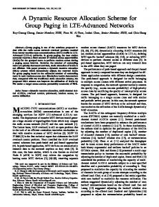
contiguous blocks of spectrum to the radio access networks (RANs), which are separated by guard bands. However, the widths of the spectrum blocks assigned are allowed to vary to allow for changing demand, as in Figure 1. This technique therefore allows spectrum to be reallocated at times when it is unused. DRiVE investigated many aspects of the performance of the contiguous DSA scheme, as described by Huschke and Leaves [3] and by Leaves et al [4][5][6]. Whilst spectrum management bodies have already mentioned issues such as spectrum trading, e.g. UK DTI [7], little work had previously been done on the potential for DSA to improve the spectrum efficiency. This paper generalises the performance of the contiguous DSA scheme, and describes some of the differences between the theoretical and practical gains in performance. THE CONTIGUOUS DSA METHOD
INTRODUCTION
A method called contiguous DSA has been developed in DRiVE to allow spectrum allocations to change over time, depending on the loads. This scheme allocates
UMTS
DVB-T 0.0
0.5
1.0
1.5
Time [Hours]
2.0
2.5
Spectrum Allocations
Offered Traffic
The current method of assigning spectrum to different radio systems is fixed allocation, where the spectrum is divided into non-overlapping blocks assigned to different radio standards. The exclusive use of spectrum solves the problem of interference between networks, with no need for co-ordination, if adequate guard bands are maintained. However, most communications networks are dimensioned to cope with a certain maximum amount of traffic, called the ‘busy hour.’ If this network utilises its spectrum fully during this time, then it is underused at all other times. Similar time-varying demands are seen with other services, e.g. broadcasting. Fixed spectrum allocation (FSA) cannot adapt to these time-varying loads, which motivates a more spectrum efficient technique called dynamic spectrum allocation (DSA). The European project DRiVE (Dynamic Radio for IP-Services in Vehicular Environments) investigated methods for DSA in a multi-radio environment, and its follow-on project, OverDRiVE (Spectrum Efficient Uni- and Multicast Services Over Dynamic Radio Networks in Vehicular Environments), furthers this concept. See Tönjes et al [1][2] for details. The OverDRiVE project objectives are: (i) improve spectrum efficiency by system coexistence in one frequency band and DSA, (ii) enable mobile multicast by UMTS enhancements and multi-radio multicast group management, and (iii) develop a vehicular router, that supports roaming into the intra-vehicular area network (IVAN).
An algorithm has been designed to implement temporal contiguous DSA, as described in [5]. The algorithm runs at set periods and the calculation of the spectrum required by each RAN is based on a prediction of the offered load until the next reallocation. There are two aspects to the prediction: a load history, which is a database of the loads seen in the past, and a time-series prediction algorithm. If unusual traffic events occur, then the load history alone is not able to adapt, leading to inappropriate spectrum allocations, so time-series prediction is used to estimate the loads. For more details on load prediction with DSA see [6]. From the load prediction, the RANs estimate the number of carriers they will require for the next time interval. They declare to the DSA if they have any currently unused carriers that can be reallocated, as a carrier can only be deactivated from a RAN if there are no ongoing calls on it. An allocation algorithm decides how the free carriers are distributed. This spectrum allocation applies until the next DSA run. To ensure that as many carriers as possible are free for DSA, all new calls are started on the carrier furthest away from the guard band between RANs, and are handed over to these carriers if they free up, making the ones nearest the guard bands available for reallocation.
0.0
UMTS Spectrum GB GB GB GB
GB
DVB-T Spectrum 0.5
1.0
1.5
2.0
Time [Hours]
Figure 1. Basic operation of contiguous DSA
2.5
is obtained. This implies that the spectrum required for each of the RANs with FSA is:
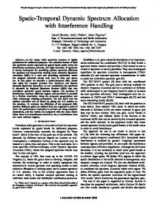
THEORETICAL DSA PERFORMANCE The operation of a temporal DSA system relies on the time-varying traffic patterns of the RANs sharing the spectrum being different, or at best uncorrelated. The work performed here considers two RANs sharing a block of spectrum: a DVB-T broadcast and a UMTS cellular system. These offer differing services, implying different traffic patterns. Consider Figure 2a where the traffic patterns for the RANs are perfectly uncorrelated (i.e. a correlation coefficient of –1), with the demands normalised to one. If the RANs had equal peak demands for the spectrum, then, for FSA, an equal block of spectrum would be required for each RAN to support its peak load. Therefore, if the RANs were to share this overall block of spectrum, then the RANs would have access to twice as much spectrum as they would with FSA, implying that they would be able to support at least twice as much traffic with DSA as FSA, in the same total block of spectrum, leading to a spectrum efficiency gain of 100%. In reality, the gain would be over 100%, due to increased trunking gain with more spectrum, but this is ignored here. Conversely, a correlation of +1 would give 0% gain, since the RANs would both require spectrum from DSA to support their peak loads simultaneously, giving no advantage compared to FSA. However, traffic correlations of –1 or +1 are unrealistic. Therefore, we consider more realistic traffic patterns, derived from actual services. This work considers a speech service over UMTS, and a multicasted video service over DVB-T. Figure 2b shows example traffic patterns, derived from extrapolation of current services. The UMTS curve is from GSM voice service demand from Almeida et al [8], and the DVB-T service is from TV viewing figures from Kiefl [9]. The potential gain obtainable by utilising DSA for two RANs can be generalised for any pair of traffic patterns. The gain of DSA is defined as the increase in traffic that can be supported in the same amount of spectrum when DSA is compared to FSA. If we have spectrum demand curves, such as in Figure 2, normalised to the RAN with the largest peak demand (note that the peak demands in each RAN do not have to be equal for this analysis to hold true), then the demands for each RAN can be represented as: D R1 = {d 1, R1 , d 2, R1 ,
K, d
n , R1
},
D R 2 = {d 1, R 2 , d 2, R 2 ,
K, d
n, R 2
}
(1)
Where: DRx = demand pattern for RAN x, dt,Rx = value of the demand for RAN x at time t, n = number of values in the demand pattern
(a) DVB-T
0.6 0.4 0.2
UMTS
0.0
Spectrum Demand
Spectrum Demand
0.8
(b)
1.0 0.8
DVB-T
4
8
12 16 Time [hours]
20
24
(2)
The spectrum required for DSA is the peak value of the cumulative demands for the two RANs, given by: S DSA = max(DR1 + DR 2 )
(3)
Where: SDSA = total spectrum required with DSA
The gain of DSA is the amount by which the spectrum demand can be increased in each RAN with DSA, such that the spectrum required equals that of FSA: iGDSA = iG DSA =
(S
FSA, R1
+ S FSA,R 2 ) − S DSA S DSA
(4)
⋅ 100
max(DR1 ) + max(DR 2 ) − max(D R1 + DR 2 ) ⋅ 100 max(DR1 + DR 2 )
(5)
Where: iGDSA = ideal gain of DSA in percent
For the pattern in Figure 2b, this gives a gain of 40.3%. Therefore, with DSA, the spectrum demands could be increased by 40% equally in each RAN in order to obtain the same user satisfaction as FSA, giving the fairest sharing of the spectrum. However, it is possible to increase the demands unequally, but obtain the required overall increase in spectrum demand. Any combination of gains is possible for the two RANs, provided the following relation is maintained: d T , R1 (G DSA, R1 + 100 ) + d T , R 2 (G DSA , R 2 + 100 ) 100
= S FSA, R1 + S FSA, R 2
(6)
Where: T = time of peak cumulative spectrum demand, GDSA,Rx = DSA gain for RAN x in percent
This affects the results since at time T the two RANs may have differing individual demands (dT,R1 & dT,R2), meaning that an equal increase in demand may not be optimum. In addition, if the two RANs do not utilise their allocated spectrum equally, e.g. if one RAN fits more users into its allocated spectrum, then to increase the overall number of satisfied users, it may not be optimum to increase the RAN’s traffic equally. This can be taken into account by considering two ratios. The first is denoted AR1:AR2, and is the ratio of the areas under the spectrum demand curves for both RANs. This gives the total spectrum demand over the whole day for each RAN. The other ratio is denoted TR1:TR2, and is the ratio of the traffic usage per unit spectrum demand. The following ratio can then be derived as the relative traffic supported by each RAN: AR1TR1 A T : R2 R2 TR1 + TR 2 TR1 + TR 2
(7)
Where: URx = traffic over RAN x
From this and the individual RAN gains, the overall performance can be calculated as a weighted average: G DSA =
G DSA, R1U R1 + G DSA, R 2U R 2
(8)
U R1 + U R 2
0.6
Where: GDSA = DSA gain in percent
0.4 0.2
UMTS
0.0 0
S FSA , R 2 = max (DR 2 )
Where: SFSA,Rx = FSA spectrum required for RAN x
U R1 : U R 2 =
It is assumed that, for FSA, the networks are dimensioned for the busy hour traffic (i.e. the peak of the traffic demand) such that a sufficient user satisfaction ratio 1.0
S FSA , R1 = max (DR1 ) ,
0
4
8
12 16 Time [hours]
Figure 2. Example time-varying traffic patterns
20
24
For Figure 2b, AR1:AR2 = 49:51. Assume that TR1:TR2 is 3:2. The value of dT,R1 = 1, and dT,R2 = 0.426, and SFSA,R1 = SFSA,R2 = 1. This allows the calculation of the potential
Gain of RAN 2 [%]
70
120
60
100
50
80
40
60
30 Ideal RAN1 vs. RAN2
40
20
Actual RAN1 vs. RAN2 Ideal RAN1 vs. Overall
20
Overall Gain [%]
140
10
Actual RAN1 vs. Overall 0
0 0
5
10
15
20
25 30 35 Gain of RAN 1 [% ]
40
45
50
55
60
Figure 3. RAN 1 gain vs. RAN 2 & overall gains
gains from DSA for the possible combinations of GDSA,R1 and GDSA,R2. Therefore, from (6) and (10): G DSA, R 2 =
57.4 − G DSA, R1
and G DSA =
0.426
29.4 ⋅ G DSA, R1 + 20.4 ⋅ G DSA, R 2
(9)
49.8
Figure 3 shows these relationships, plotted against GDSA,R1. The solid lines show the trends from (9). Notice that when the RAN 1 gain is 40%, so is the RAN 2 and overall gains, as predicted by (5). The overall gain line increases past 40% and goes as high as 55% for low RAN 1 gains. However, the solid lines are not attainable in reality, because at low RAN 1 gains (