choosing between alternative courses of action when the conse- quences resulting ... was presented at the IEEE Systems Science and Cybernetics Con- ference ...
200
IEEE TRANSACTIONS ON SYSTEMS SCIENCE AND CY13ERNETICS, VOL.
A
Tutorial
Introduction
SSC-4,
NO.
3, SEPTEMLIER 1968
to Decision Theory
D. WARNER NORTH
Abstract-Decision theory provides a rational framework for choosing between alternative courses of action when the consequences resulting from this choice are imperfectly known. Two streams of thought serve as the foundations: utility theory and the inductive use of probability theory. The intent of this paper is to provide a tutorial introduction to this increasingly important area of systems science. The foundations are developed on an axiomatic basis, and a simple example, the "anniversary problem," is used to illustrate decision theory. The concept of the value of information is developed and demonstrated. At times mathematical rigor has been subordinated to provide a clear and readily accessible exposition of the fundamental assumptions and concepts of decision theory. A sampling of the many elegant and rigorous treatments of decision theory is provided among the references.
INTRODUCTION
THE NECESSITY of makinig decisions in the face of uncertainty is an integral part of our lives. We must act without knowing the consequeinces that will result from the action. This uncomfortable situation is particularly acute for the systems engineer or manager who must make far-reaching decisions oIn complex issues in a rapidly changing technological environment. Uncertainty appears as the dominant consideration in many systems problems as well as in decisions that we face in our personal lives. To deal with these problems oii a rational basis, we must develop a theoretical structure for decisiotn making that includes uncertainity. Confronting uncertainty is Inot easy-. We naturally try to avoid it; sometimes we even pretend it does not exist. Our primitive ancestors sought to avoid it by consulting soothsayers and oracles who would "reveal" the uncertain future. The methods have changed: astrology and the reading of sheep entrails are somewhat out of fashion today, but predictions of the future still abound. Much current scientific effort goes into forecasting future economic and technological developments. If these predictions are assumed to be completely accurate, the uncertainty in many systems decisions is eliminated. The outcome resulting from a possible course of action may then be presumed to be known. Decision making becomes an optimization problem, and techniques such as mathematical programming may be used to obtain a solution. Such problems may be quite difficult to solve, but this difficulty should Manuscript received M\ay 8, 1968. An earlier version of this paper
was presented at the IEEE Systems Science and Cybernetics Conference, Washington, D.C., October 17, 1966. This research was sup-
ported in part by the Graduate Cooperative Fellowship Program of the National Science Foundation at Stanford University, Stanford, Calif. The author is with the Systems Sciences Area, Stanford Research Institute, MTenlo Park, Calif. 94025.
not obscure the fact that they represent the limiting case of perfect predictions. It is often tempting to assume perfect predictions, but in so doing we may be eliminatinig the most important features of the problem.' We should like to include in the analysis not just the predictions themselves, but also a measure of the confidence we have in these predictions. A formal theory of decision making must take uncertainty as its departure point and regard precise knowledge of outcomes as a limiting special case. Before we begin our exposition, we will clarify our point of view. We shall take the enginieering rather than the purely sc ientific viewpoint. We are not observing the way people make decisions; rather we are participanits in the decision-making process. Our concerin is in actually making a decision, i.e., making a choice between alternative ways of allocating resources. We must assume that at least two distinct alternatives exist (or else there is 11o element of choice and, consequently, no problem). Alternatives are distinct only if they result in different (uncertain) rewards or penalties for the decision maker; once the decisioni has been made and the uncertainty resolved, the resource allocation can be changed only by incurring some penalty. What can we expect of a general theory for decision making under uncertainty? It should provide a framework in which all available information is used to deduce which of the decision alternatives is "best" according to the decision maker's preferences. But choosing an alternative that is consistent with these preferences and present knowledge does not guarantee that we will choose the alternative that by hindsight turns out to be most profitable. We might distiniguish between a good decision and a good outcome. We are all familiar with situations in which careful management and extensive planning produced poor results, while a disorganized and badly managed competitor achieved spectacular success. As an extreme example, place yourself in the position of the company president who has discovered that a valuable and trusted subordinate whose past judgment had proved unfailingly, accurate actually based his decisions upon the advice of a gypsy fortune teller. Would you promote this man or fire him? The answer, of course, is to fire him and hire the gypsy as a consultant. The availability of such a clairvoyant to provide perfect information would make deci-sion theory unnecessary. But we should not confuse the two. Decision theory is not a substitute for the fortune teller. It is rather a procedure that takes account of all available information to give us the best possible logical I For further discussion of this point, see Howard [10] and Klein and Meckling [141.
201
NORTH: INTRODUCTION TO DECISION THEORY
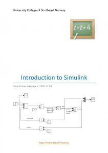
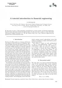
POSSIBLE OUTCOMES DECISION ALTERNATIVES
IT IS YOUR ANNIVERSARY
IT IS NOT YOUR
ANNIVERSARY
BUY FLOWERS
DO NOT BUY FLOWERS
Fig. 1. Anniversary problem payoff matrix.
BUY FLOWERS
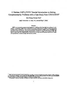
decision. It will minimize the consequences of getting an unfavorable outcome, but we cannot expect our theory to shield us from all "bad luck." The best protection we have against a bad outcome is a good decision. Decision theory may be regarded as a formalization of common sense. Mathematics provides an unambiguous language in which a decision problem may be represented. There are two dimensions to this representation that will presently be described: value, by means of utility theory, and information, by means of probability theory. In this representation, the large and complex problems of systems analysis become conceptually equivalent to simple problems in our daily life that we solve by "common sense." We will use such a problem as an example. You are driving home from work in the evening when you suddenly recall that your wedding anniversary comes about this time of year. In fact, it seems quite probable (but not certain) that it is today. You can still stop by the florist shop and buy a dozen roses for your wife, or you may go home empty-handed and hope the anniversary date lies somewhere in the future (Fig. 1). If you buy the roses and it is your anniversary, your wife is pleased at what a thoughtful husband you are and your household is the very epitome of domestic bliss. But if it is not your anniversary, you are poorer by the price of the roses and your wife may wonder whether you are trying to make amends for some transgressioil she does not know about. If you do not buy the roses, you will be in the clear if it is not your anniversary; but if it is, you may expect a temper tantrum from your wife and a two-week sentence to thedoghouse. What do you do? We shall develop the general tools for solving decision problems and then return to this simple example. The reader might consider how he would solve this problem by ''common sense" and then compare his reasoning with the formal solution which we shall develop later (Fig. 2). THE MACHINERY OF DECISION MAKING
//j DO NOT BUY FLOWERS
X
DECISION POINT
o
RESOLUTION OF UNCERTAINTY
STATUS QUO
Fig. 2. Diagram of anniversary decision.
Utility Theory The first stage in setting up a structure for decision making is to assign numerical values to the possible outcomes. This task falls within the area covered by the modern theory of utility. There are a number of ways of developing the subject; the path we shall follow is that of Luce and Raiffa [16 ].2 The first and perhaps the biggest assumption to be made is that any two possible outcomes resulting from a decision can be compared. Given any two possible outcomes or prizes, you can say which you prefer. In some cases you might say that they were equally desirable or undesirable, and therefore you are indifferent. For example, you might prefer a week's vacation in Florida to a season ticket to the symphony. The point is not that the vacation costs more than the symphony tickets, but rather 2 The classical reference on modern utility theory is von Neumann and Morgenstern [22]. A recent survey of the literature on utility theory has been made by Fishburn [5].
2029
IEEE TR
that you prefer the vacationi. If you were offered the vacation or the symphony tickets on a nonnegotiable basis, you would choose the vacation. A reasonable extension of the existence of y-our preference among outcomes is that the preferenice be transitive; if you prefer A to B and B to C, then it follo(ws that Xyou prefer A to C.3 The second assumption, originated by von NXeumann arid Morgenstern [22], forms the core of modern utilitytheory: you can assign preferences in the same mariner to lotteries involving prizes as you can to the prizes themselves. Let us define what we meani by a lottery. Imaginie a poitnter that spins in the center of a circle divided inito two regions, as showni in Fig. 3. If you spin the pointer and it lands in region I, you get prize A; if it lands in region II, you get prize B. We shall assume that the poiniter is spun in such a way that, when it stops, it is equally likely to be pointing in any given direction. The fraction of the circumference of the circle in region I will be denoted P, and that in region II as 1 - P. Then from the assumption that all directionis are equally likelv, the probability that the lottery gives you prize A is P, and the probability that you get prize B is 1 - P. We shall denote such a lottery as (P,A;1 - P,B) and represent it, by- F'ig. 4. Now suppose you are asked to state your preferences for prize A, prize B, and a lottery of the above type. Let us assume that y-ou prefer prize A to prize B. Then it would seem natural for you to prefer prize A to the lottery, (P,A;1 - P,B), between prize A. arid prize B, arid to prefer this lottery betweein prize A arid prize B to prize B for all probabilities P between 0 and 1. You would rather have the preferred prize A than the lottery, and you would rather have the lottery than the inferior prize B. Furthermore, it seems natural that, given a choice betweein two lotteries involving prizes A and B, you would choose the lottery with the higher probability of getting the preferred prize A, i.e., you prefer lottery (P,A;1 - P,B) to (P',A; 1-P',B) if anid only if P is greater thai P'. The final assumptions for a theory of utility are not quite so natural and have been the subject, of much discussion. Nonetheless, they seem to be the most reasonable basis for logical decision makiing. The third assumption is that there is no intrinsic reward in lotteries, that is, "nio fun in gambling." Let us consider a compound lottery, a lottery in which at least, one of the prizes is riot an outcome but another lottery among outcomes. For example, eonisider the lottery (P,A;1 - P,(P',B;1 - P',C)). If the pointer of Fig. 3 lands in region I, you get prize A; if it lands in region II, you receive another lottery that has I Suppose not: you would be at least as happy with C as with A. Then if a little man in a shabby overcoat came up and offered youl C instead of A, you would presumably accept. Now you have C; and since you prefer B to C, you would presumably pay a sum of money to get B instead. Once you had B, you prefer A; so you would pay the man in the shabby overcoat some more money to get A. Butt now you are back where you started, with A, and the little mani in the shabby overcoat walks away counting your money. Given that youi accept a standard of value such as money, transitivity prevents youi from becoming a "money ptump."
\NSA\CTIONS ON
SYST'EMS SCIENCE
AND
CYBERNETICS, SEPTEMBER 196S
pKI Fig. 3. A lottery. P
A
I -P
B
Fig. 4. Lottery diagram.
A
A
P C(I- P)'
B
IP
(I-P)
pIP
(I-P) C
C
COMPOUND LOTTERY
B
EQUIVALENT SIMPLE LOTTERY
Fig. ,. "No fun in gamblitig."
different, prizes and perhaps a differenit divisioin of the circle (Fig. 5). If you spini the second pointer you will receive prize B or prize C, depending on where this pointer lands. The assumption is that subdividing region II into two parts whose proportions correspond to the probabilities P' arid 1 - P' of the second lottery creates ain equivalent simple lottery in which all of the prizes are outcomes. According to this third assumptioii, you can decompose a compound lottery by multiplying the probabilit) of the lottery prize in the first lottery by the probabilities of the inidividual prizes in the second lottery; you should be indifferenit betweein (P,A;1 -IP,(P',B;1 - ', C)) anid (P,A;P' - PP',B;1 - P- P' + PP',C). In other words, your preferences are riot affected by the wayin which the uncertainty is resolved bit by bit, or all at once. There is no value in the lotterv itself; it does riot matter whether you spin the pointer oince or twice. Fourth, we make a continuity assumption. Considei three prizes, A, B, arid C. You prefer A to C, and C to B (and, as we have pointed out, you will therefore prefer A to B). We shall assert that there must, exist some probability P so that yrou are indifferetnt, to receiving prize C or
203
NORTH: INTRODUCTION TO DECISION THEORY
the lottery (P,A;1 - P,B) between A and B. C is called the certain equivalent of the lottery (P,A;1 - P,B), an11d on the strength of our "no fun in gambling" assumptioit, we assume that interchangiing C and the lottery (P,A;1 - P,B) as prizes in some compound lottery does iiot change your evaluation of the latter lottery. We have not assumed that, given a lottery (P,A;1 - P,B), there exists a Prize C intermediate in value between A and B so that you are indifferent between C and (P,A;1 - P,B). Inistead we have assumed the existence of the probability P. Given prize A preferred to prize C preferred to prize B, for some P between 0 and 1, there exists a lottery (P,A; 1 - P,B) such that you are indifferenit between this lottery and Prize C. Let us regard the circle in Fig. 3 as a "pie" to be cut into two pieces, region I (obtain prize A) and region II (obtain prize B). The assumption is that the "pie" can be divided so that you are indifferent as to whether you receive the lottery or intermediate prize C. Is this continuity assumption reasonable? Take the following extreme case: A = receive $1; B = death; C = receive nothing (status quo). It seems obvious that most of us would agree A is preferred to C, and C is preferred to B; but is there a probabilitv P such that we would risk death for the possibility of gaining $1? Recall that the probability P can be arbitrarily close to 0 or 1. Obviously, we would not engage in such a lottery with, say, P = 0.9, i.e., a 1-in-10 chance of death. But suppose P = 1 - 1 X 10-50, i.e., the probability of death as opposed to $1 is not 0.1 but 10 -50. The latter is considerably less than the probability of being stru(ck onI the head by a meteor in the course of going out to pick up a $1 bill that someone has dropped on your doorstep. MAost of us would not hesitate to pick up the bill. Even in this extreme case where death is a prize, we conclude the assumption is reasonable. We can summarize the assumptions we have made into the followiing axioms. A, B, C are prizes or outcomes resulting from a decision.
3) (P,A;1 - P,(P',B;1 - P',C)) (P,A;P' - PP',B; 1 - P - P' + PP',C), i.e., there is "nIo fun in gambling." 4) If A > C > B, there exists a P with 0 < P < 1 so that -
C,(P,A;I1- P,B) i.e., it makes no difference to the decision maker whether C or the lottery (P,A;1 - P,B) is offered to him as a prize.
Under these assumptions, there is a concise mathematical representation possible for preferences: a utility function u( ) that assigns a number to each lottery or prize. This utility function has the following properties:
u(A) > u(B) if and only if A > B if C
(P,A;1 -P,B), then u(C) = P u(A) + (1 - P) u(B)
(1) (2)
i.e., the utility of a lottery is the mathematical expectation of the utility of the prizes. It is this "expected value" property that makes a utility function useful because it allows complicated lotteries to be evaluated quite easily. It is important to realize that all the utility function does is provide a means of consistently describing the decision maker's preferences through a scale of real numbers, providing these preferences are consistent with the previously mentioned assumptions 1) through 4). The utility function is no more than a means to logical deduction based on given preferences. The preferences come first and the utility function is only a convenieint means of describing them. We can apply the utility conicept to almost any sort of prizes or outcomes, from battlefield casualties or achievements in space to preferences for Wheaties or Post Toasties. All that is necessary is that the decision maker have unambiguous preferences and be willing to accept the basic assumptions. In many practical situations, however, outcomes are in terms of dollars and cents. What does the utility concept mean here? For an example, let us suppose you were offered the following lottery: a coin will be flipped, and if you guess the outcome correctly, you gain $100. If you guess incorrectly, you get nothing. We shall assume you feel that the coin has an equal probability of coming up heads or tails; it corresponds to the "lottery" which we Notation: have defined in terms of a pointer with P = 1/2. How means "is preferred to;" much would you pay for such a lottery? A common answer A > B means A is preferred to B; to this academic question is "up to $50," the average ormeans "is indifferent to;" expected value of the outcomes. When real money is inA B means the decision maker is indifferent be- volved, however, the same people tend to bid considerably tween A and B. lower; the average bid is about $20.4 A group of Stanford University graduate students was actually confronted with Utility Axioms: a $100 pile of bills and a 1964 silver quarter to flip. The 1) Preferences can be established between prizes and average of the sealed bids for this game was slightly under lotteries in an unambiguous fashion. These preferences are $20, and only 4 out of 46 ventured to bid as high as $40. transitive, i.e., (The high bidder, at $45.61, lost and the proceeds were for a class party.) These results are quite typical; used A>B, B>C impliesA>C in fact, professional engineers and maniagers are, if anvA B, B-C impliesA-C. 2) If A > B, then (P,A;1 - P,B) > (P',A;1 - P',B) if 4Based on unpublished data obtained by Prof. R. A. Howard of and only if P > P'. Stanford University, Stanford, Calif.
204
IEEE TRANSACTIONS ON SYSTEMS SCIENCE AND CYBERNETICS, SEPTEMBER 1968
thing, more conservative in their bids than the less affluent students. The lesson to be learned here is that, by and large, most people seem to be averse to risk in gambles involving what is to them substantial loss. They are willing to equate the value of a lottery to a sure payoff or certain equivalent substantially less than the expected value of the outcomes. Similarly, most of us are willing to pay more than the expected loss to get out of an unfavorable lottery. This fact forms the basis of the insurance industry. If you are very wealthy and you are confronted with a small lottery, you might well be indifferent to the risk. An unfavorable outcome would not deplete your resources, and you might reason that you will make up your losses in future lotteries; the "law of averages" will come to your rescue. You then evaluate the lottery at the expected value of the prizes. For example, the (1/2, $0; 1/2, $100) lottery would be worth 1/2($0) + 1/2($100) = $50 to you. Your utility function is then a straight line, and we say you are an "expected value" decision maker. For lotteries involving small prizes, most individuals and corporations are expected value decision makers. We might regard this as a consequeiice to the fact that any arbitrary utility curve for money looks like a straight line if we look at a small enough section of it. Only when the prizes are substantial in relation to our resources does the curvature become evident. Then an unfavorable outcome really hurts. For these lotteries most of us become quite risk averse, and expected value decision making does niot accurately reflect our true preferences. Let us now describe one way you might construct your owin utility curve for money, say, in the amounts of $0 to $100, in addition to your present assets. The utility function is arbitrary as to choice of zero point and of scale factor; changing these factors does not lead to a change in the evaluation of lotteries using properties (1) and (2). Therefore, we can take the utility of $0 as 0 and the utility of $100 as 1. Now determine the minimum amount you would accept in place of the lottery of flipping a coin to determine whether you receive $0 or $100. Let us say your answer is $27. Now determine the certain equivalent of the lotteries (1/2, $0; 1/2, $27), and (1/2, $27; 1/2, $100), and so forth. We might arrive at a curve like that shown in Fig. 6. We have simply used the expected value property (2) to construct a utility curve. This same curve, however, allows us to use the same expected utility theorem to evaluate new lotteries; for example, (1/2, $30; 1/2 $80). From Fig. 6, u($30) = 0.54, u($80) = 0.91, and therefore 1/2 u($30) + 1/2 u($80) = u(x) > x = $49. If you are going to be consistent with the preferences you expressed in developing the utility curve, you will be indifferent between $49 and this lottery. -Moreover, this amouint could have been determined from your utility curve by a subordinate or perhaps a computer program. You could send your agent to make decisions on lotteries by using your utility curve, and he would make them to reflect your preference for amounts in the range $0 to $100.
1.00
0.75
-' 0.50
0.25
0 0
20
Fig. 6. Utility
40 60 MONEY- dollars
cuirve for money:
80
100
$0 to $100.
Even without such a monletary represeintationi, we caii always construct a utility function oin a fiinite set of outcomes by using the expected value property (2). Let us choose two outcomes, one of which is preferred to the other. If we set the utilities arbitrarily at 1 for the preferred outcome and 0 for the other, we can use the expected value property (2) of the utility function to determine the utility of the other prizes. This procedure will always wor-k so long as our preferences obey the axioms, but it may be unwieldy in practice because we are asking the decision maker to assess simultaneously his values in the absenice of uncertainty and his preference among risks. The value of some outcome is accessible onily by reference to a lottery involving the two "reference" outcoomes. For example, the reference outcomes in the aniniversary problem might be "domestic bliss" = 1 and "doghouse" = 0. We could then determine the utility of "status quo" as 0.91 since the husband is indifferent between the outcome "status quo" and a lottery in which the chances are 10 to 1 of "domestic bliss" as opposed to the "doghouse." Similarly, we might discover that a utility of 0.667 should be assigned to "suspicious wife and $6 wasted on roses," siince our friend is ilndifferent between this evenituality and a lottery in which the probabilities are 0.333 of "doghouse" and 0.667 of "domestic bliss." Of course, to be consistenit with the axioms, our friend must be indifferent between "suspicious wife, etc. ," and a 0.73 probability of "status quo" and a 0.27 probability of "doghouse." If the example included additional outcomes as well, he might find it quite difficult to express his preferences among the lotteries in a maiinner consistent with the axioms. It may be advisable to proceed in two stages; first, a numerical determination of value ill a risk-free situation, and then an adjustment to this scale to include preference toward risk. Equivalent to our first assumption, the existence of transitive preferences, is the existence of some scale of value by which outcomes may be rankied; A is preferred to B if and only if A is higher in value than B. The numericCal
NORTH: INTRODUCTION TO DECISION THEORY
structure we give to this value is not important since a monotonic transformation to a new scale preserves the ranking of outcomes that corresponds to the original preferences. No matter what scale of value we use, we can construct a utility function on it by usiIng the expected value property (2), so long as our four assumptions hold. We may as well use a standard of value that is reasonably intuitive, and in most situations money is a convenient standard of economic value. We can then find a monetary equivalenit for each outcome by determining the point at which the decision maker is indifferent between receiving the outcome and receiving (or paying out) this amount of moliey. In addition to conceptual simplicity, this procedure makes it easy to evaluate new outcomes by providing an intuitive scale of values. Such a scale will become necessary later on if we are to consider the value of resolving uncertainty. We will return to the anniversary decision and demonstrate how this two-step value determination procedure may be applied. But first let us describe how we shall quantify uncertainty. The Inductive Use of Probability Theory We now wish to leave the problem of the evaluation of outcomes resulting from a decision and turn our attention to a means of encoding the information we have as to which outcome is likely to occur. Let us look at the limiting case where a decision results in a certain outcome. We might represent an outcome, or an event, which is certain to occur by 1, and an event which cannot occur by 0. A certain event, together with another certain event, is certain to occur; but a certain event, together with an impossible event, is certain not to occur. Mlost engineers would recognize the aforementioned as simple Boolean equations: 1 1 = 1, 1 .0 = 0. Boolean algebra allows us to make complex calculations with statements that may take on only the logical values "true" and "false." The whole field of digital computers is, of course, based on this branch of mathematics. But how do we handle the logical "maybe?" Take the statement, "It will rain this afternoon." We cannot now assign this statement a logical value of true or false, but we certainly have some feelings on the matter, and we may even have to make a decision based on the truth of the statement, such as whether to go to the beach. Ideally, we would like to generalize the inductive logic of Boolean algebra to include uncertainty. We would like to be able to assign to a statement or an event a value that is a measure of its uncertainty. This value would lie in the range from 0 to 1. A value of 1 indicates that the statement is true or that the event is certain to occur; a value of 0 indicates that the statement is false or that the event cannot occur. WVe might add two obvious assumptions. We want the value assignments to be unambiguous, and we want the value assignments to be independent of any assumptions that have not been explicitly introduced. In particular, the value of the statement should depend on its content, not on the way it is presented. For example, "It will rain this
205
morning or it will rain this afternoon," should have the same value as "It will rain today." These assumptions are equivalent to the assertion that there is a function P that gives values between 0 and 1 to events ("the statement is true" is an event) and that obeys the following probability axioms.5 Let E and F be events or outcomes that could result from a decision: 1) P(E) > 0 for any event E; 2) P(E) = 1, if E is certain to occur; 3) P(E or F) = P(E) + P(F) if E and F are mutually exclusive events (i.e., only one of them can occur). E or F means the event that either E or F occurs. We are in luck. Our axioms are identical to the axioms that form the modern basis of the theory of probability. Thus we may use the whole machinery of probability theory for inductive reasoning. Where do we obtain the values P(E) that we will assign to the uncertainty of the event E? We get them from our own minds. They reflect our best judgment on the basis of all the information that is presently available to us. The use of probability theory as a tool of inductive reasoning goes back to the beginnings of probability theory. In Napoleon's time, Laplace wrote the following as a part of his introduction to A Philosophical Essay on Probabilities ([15], p. 1): Strictly speaking it may even be said that nearly all our knowledge is problematical; and in the small numbers of things which we are able to know with certainty, even in the mathematical sciences themselves, the principal means for ascertaining truth-induction and analogy-are themselves based on probabilities ....
Unfortunately, in the years following Laplace, his writings were misinterpreted and fell into disfavor. A definition of probability based on frequency came into vogue, and the pendulum is only now beginning to swing back. A great many modern probabilists look on the probability assigned to an event as the limiting fraction of the number of times an event occurred in a large number of independent repeated trials. We shall not enter into a discussion of the general merits of this viewpoint on probability theory. Suffice it to say that the situation is a rare one in which you can observe a great many independent identical trials in order to assign a probability. In fact, in decision theory we are often interested in events that will occur just once, For us, a probability assessment is made on the basis of a state of mind; it is not a property of physical objects to be measured like length, weight, or temperature. When we assign the probability of 0.5 to a coin coming up heads, or equal probabilities to all possible orientations of a pointer, we may be reasoning on the basis of the symmetry of the I Axioms 1) and 2) are obvious, and 3) results from the assumption of invariance to the form of data presentation (the last sentence in the preceding paragraph). Formal developments may be found in Cox [3], Jaynes [121, or Jeffreys [131. A joint axiomatization of both probability and utility theory has been developed by Savage [20].
206
IEEE TRANSACTIONS ON SYSTEMS SCIENCE AND CYBERNETICS, SEPTEMBER 1968
physical object. There is nO reason to suppose that one side of the coin\iill be favored over the other. But the physical symmetry of the coin does not lead immediately to a probability assiginmenit of 0.5 for heads. For example, consider a coin that is placed on a drum head. The drum head is struck, atnd the coin bounces into the air. Will it land heads up half of the time? We might expect that the probability of heads would depend on which side of the coin was up iniitially, how hard the drum was hit, anid so forth. The probability of heads is not a physical parameter of the coin; we have to specify the flipping system as wvell. But if we kiiew exactly how the coin were to be flipped, we could calculate from the laws of mechanics whether it would land heads or tails. Probability enters as a means of describiing our feelings about the likelihood of heads when our kinowledge of the flipping system is not exact. We must conclude that the probability assignment depenids on our present state of kniowledge. The most importanit consequence of this assertion is that probabilities are subject to change as our iniformation improves. In fact, it even makes sense to talk about probabilities of probabilities. A few years ago we might have assigned the value 0.5 to the probability that the surface of the moon is covered by a thick layer of dust. At the time, we might have said, "We are 90 percent certain that our probability assignment after the first successful Surveyor probe will be less than 0.01 or greater than 0.99. We expect that our uncertainty about the compositioIn of the mooin's surface will be largely resolved." Let us conclude our discussion of probability theory with an example that will introduce the means by which probability distributions are modified to include new information: Bayes' rule. We shall also introduce a useful notationi. We have stressed that all of our probability assigniments are going to reflect a state of information in the mind of the decision maker, and our notation shall indicate this state of information explicitly. Let A be an evenit, and let x be a quantity about which we are uncertain; e.g., x is a random variable. The values that x may assume may be discrete (i.e., heads or tails) or continuous (i.e., the time an electronic component will ruin before it fails). We shall denote by {A|S} the probability assigned to the event A on the basis of a state of information S, and by {xjS} the probability that the random variable assumes the value x, i.e., the probability mass function for a discrete random variable or the probability density fuinetion for a continuous random variable, given a state of informatioin S. If there is confusion between the random variable and its value, we shall write {x = x01S}, where x denotes the random variable and x0 the value. We shall assume the random variable takes on some value, so the probabilities must sum to 1:
value, or the average of the random variable over its probability distributioni, is
(xjS)
X{.xs}.
=
(4)
One special state of iniformation will be used over anid over again, so we shall need a special name for it. This is the iinformation that we niow possess on the basis of our prior knowledge and experience, before we have done aIny special experimenting or sampling to reduce our unicertainty. The probability distribution that we assigni to values of an uncertaii (quantity on the basis of this prior state of information (denoted g) will be referred to as the "prior distribution" or simply the "prior." Nowv let us consider a problem. Most of us take as axiomatic the assignment of 0.5 to the probability of heads on the flip of a coin. Suppose we flip thumbtacks. If the thumbtack lands with the head up and poinit dowil, we shall deniote the outcome of the flip as "heads." If it laIlds with the head down and the point up, we shall denote the outcome as "tails." The question which we must answer is, "What is p, the probability of heads in flipping a thumbtack?" We will assume that both thumbtack anid means of flipping are sufficiently standardized so that wve may expect that all flips are independent and have the same probability for coming up heads. (Formally, the flips are Bernoulli trials.) Then the long-run fractioin of heads may be expected to approach p, a well-definied number that at the moment we do not know. Let us assign a probability distribution to this uncertain parameter p. We are all familiar with thumbtacks; we have no doubt dropped a few on the floor. Perhaps we have some experience with spilled carpet tacks, or coin flipping, or the physics of falling bodies that we believe is relevanit. We want to encode all of this prior information inito the form of a probability distribution on p. This task is accomplished by using the cumulative distribution functioin, {p < polg}, the probability that the parameter p will be less than or equal to some specific value of the parameter po. It may be convenienit to use the complementary cumulative
lp > polg}
=
1
-
lp < Pol8}
and ask questions such as, "What is the probability that p is greater than Po = 0.5?" To make the situation easier to visualize, let us introduce Sam, the neighborhood bookie. We shall suppose that we are forced to do business with Sam. For some value Po between 0 and 1, Sam offers us two packages: Package 1: If measurement of the long runi fractioin of heads p shows that the quantity is less than or equal to po, then Sam pays us $1. If p > po, then we pay Sam $1. f {xIS} = 1. (3) Package 2: We divide a circle into two regions (as showni in Fig. 3). Region I is defined by a fraction P of the circumf is a generalized summation operator represeniting ference of the circle, and the remainder of the circle consummation over all discrete values or integration over all stitutes region II. Now a pointer is spun in such a way contiinuous values of the random variable. The expected that when it stops, it is equally likely to be pointing in anyv
207
NORTH: INTRODUCTION TO DECISION THEORY
given direction. If the pointer stops in region I, Sam pays us $1; if it lands in region II, we pay Sam $1. Sam lets us choose the fraction P in Package 2, but then he chooses which package we are to receive. Depending on the value of po, these packages may be more or less attractive to us, but it is the relative rather than the absolute value of the two packages that is of interest. If we set P tco be large, we might expect that Sam will choose package 1, whereas if P is small enough, Sam will certainly choose package 2. Sam wishes (just as we do) to have the package with the higher probability of winning $1. (Recall this is our secoind utility axiom.) We shall assume Sam has the same information about thumbtacks that we do, so his probability assiginments will be the same as ours. The assumptioni [utility axiom 4) ] is that givein po, we can find a P such that Packages 1 and 2 represeint equivalent lotteries, so P = {p < pol8}F6 The approach is similar to the well-known method of dividinig an extra dessert between two small boys: let one divide and the other choose. The first is motivated to make the division as even as possible so that he will be indifferent as to which half he receives. Suppose Sam starts at a value po = 0.5. We might reason that since nails always fall oIn the side (heads), and a thumbtack is intermediate betweeni a coin and a nail heads is the more likely orientation; but we are not too sure; we have seen a lot of thumbtacks come up tails. After some thought, we decide that we are indifferent about which package we get if the fraetion P is 0.3, so {p < 0.518} = 0.30. Sam takes other values besides 0.5, skipping around in a random fashion, i.e., 0.3, 0.9, 0.1, 0.45, 0.8, 0.6, etc. The curve that results from the initerrogation might look like that shown in Fig. 7. By his method of randomly skipping around, Sam has eliminated aniy bias in our true feelings that resulted from an uncoinscious desire to give answers consistent with previous points. In this fashion, Sam has helped us to establish our prior distribution on the parameter p. We may derive a probability density function by takiing the derivative of the cumulative distribution function (Fig. 8): {pJ&} = (dldpo) {p < pol}. Now supposing we are allowed to flip the thumbtack 20 times and we obtain 5 heads aind 15 tails. How do we take account of this new data iii assigning a probability distribution based on the inew state of information, which we denote as 8, E: our prior experience g plus E, the 20-flip experiment? We will use oine of the oldest (1763) results of probability theory, Bayes' rule. Consider the prior probability that p will take on a specific value and the 20-flip experiment E will have a certain specific outcome (for example, p = 0.43; E = 5 heads, 15 tails). Now we can write this joint probability in two ways:
{p,E18}
=
{pJE,&} {EZ8}
(5)
6 We have equated the subjective probability that summarized our information about thumbtacks to the more intuitive notion of probability based on symmetry (in Package 2). Such a two-step approach to probability theory has been discussed theoretically by Anscombe and Aumann [1].
1.0
T
1.01-
z\ :VALUES OBTAINED THROUGH SAM'S INTERROGATION
ti3
8P 0.5
VI
00
1