Sep 25, 2015 - the virtual reality head-mounted display Oculus Rift and the motion controller Razer .... The Oculus Rift provides a 3d view of the VR scene and allows to ..... https://developer.oculus.com/downloads/pc/0.5.0.1- beta/Oculus SDK ...
BW-CAR Symposium on Information and Communication Systems (SInCom) 2015
A Virtual-Reality 3d-Laser-Scan Simulation Malvin Danhof, Tarek Schneider, Pascal Laube, Georg Umlauf Institute for Optical Systems, University of Applied Sciences Constance, Germany
hand-held laser scanner like the FARO Edge ScanArm (Fig. 1). Using this approach we can compute 3d point clouds of CAD models using a virtual laser scanner with a man-made scan structure. This paper is laid out as follows: First we describe our experimental setup and the used peripherals in Chapter II. Chapter III outlines parameters of the scanning simulation and the used data structures. We then explain the process of raycasting for triangle meshes in Chapter IV and for b-spline surfaces in Chapter V. Results are presented in Chapter VI.
Abstract—We present a 3d-laser-scan simulation in virtual reality for creating synthetic scans of CAD models. Consisting of the virtual reality head-mounted display Oculus Rift and the motion controller Razer Hydra our system can be used like common hand-held 3d laser scanners. It supports scanning of triangular meshes as well as b-spline tensor product surfaces based on high performance ray-casting algorithms. While point clouds of known scanning simulations are missing the man-made structure, our approach overcomes this problem by imitating real scanning scenarios. Calculation speed, interactivity and the resulting realistic point clouds are the benefits of this system.
I. I NTRODUCTION In science and industry 3d laser scanners are widely used to acquire 3d point data of real world objects. The result of a scanning process is a 3d point cloud. Often a CAD representation of these point clouds needs to be recovered for the subsequent processing. This task is performed by the reverse engineering process. Thus, the quality of the CAD representation depends on the chosen reverse engineering process. Evaluating reverse engineering algorithms is only possible if a large set of point clouds is available. To acquire these points clouds CAD models are scanned virtually. There are two reasons for this approach. First, we often lack enough suitable physical objects to scan and, second, point clouds of hand-scanned physical objects often lack corresponding CAD information. However, point clouds of hand-scanned physical objects and synthetically generated point clouds differ heavily in their structure in terms of scan-strategy and scan-path. Since each human operator has a different scan-strategy and scan-path, the resulting point clouds differ much in structure, even if the same object was scanned. On the one hand this structure is not completely random, on the other hand there is no good model for the human scanning procedure. For a fair evaluation of reverse engineering algorithms with realistic data this man-made structure must be incorporated into the data. To generate scans of CAD models Fig. 1: FARO ScanArm that capture this man-made structure we Edge propose a virtual reality (VR) scanner (www.faro.com, setup. We present a method to generate 09/25/2015)
A. Related Work The two most commonly used methods for high accuracy 3d scanning are laser scanners and structured light scanners. While hand-held laser scanners project a laser line onto the object surface structured light laser scanners project a pattern of light. Especially since the Michelangelo Project [1] laser scanning systems have received increasing attention. Resulting point clouds are used in numerous research fields. Ip and Gupta [2] are retrieving matching CAD models by using partial 3d point clouds. They use real and synthetic point clouds. To generate the synthetic point clouds CAD surfaces are evaluated at random parameters. Mitra et al. [3] register two point clouds by minimization of the squared distance between the underlying surfaces. They use synthetic point clouds from random evaluation with an unspecified noise. Bernardini and Bajaj [4] use synthetic point clouds generated by sampling a surface uniformly for an automatic reconstruction process. In [5] Tagliasacchi et al. extract curve skeletons from incomplete point clouds. They use a bounding sphere around a CAD model at its center to get different viewpoints. These viewpoints are used for orthographic ray casting from a uniform grid. A very similar approach is used in [6] where a fan of rays with origin on a bounding sphere is swept along the model surface from different viewpoints. However, all these approaches do not capture a realistic scan structure. The application of VR is widespread in various scientific areas. Especially in medical research VR has a huge potential using it for surgery trainings [7] or the medication in occupational therapy [8]. In the future, there will be many different applications of virtual or augmented reality simulations. A collaborative approach to develop those applications is given by [9] which also contains a collection of motion control techniques. Numerous different tools are available and individual techniques should be selected according to a concrete target application at hand.
3d point clouds from CAD models consisting of triangle meshes and b-spline tensor product surfaces with a simulated hand-held laser scanner in a VR environment. Our goal is to create a realistic simulation of the scanning process with a
68
BW-CAR Symposium on Information and Communication Systems (SInCom) 2015
II. E XPERIMENTAL SETUP For the simulation of a hand-held 3d laser scanner we propose a VR environment. The structure of the synthetic point clouds generated in this VR is similar to man-made scans of physical objects due to the manual scanning process (Figure 2). The virtual scene consists of a workshop with a table, that carries the CAD model, and a virtual model of the scanner, see Figure 3.
Fig. 3: The virtual scene.
Fig. 4: Left: Oculus Rift (www.giga.de, 09/25/2015), Right: Razer Hydra (www.roadtovr.com, 09/25/2015) Fig. 2: VR setup. within a cone with axis D and aperture angle ϕ. Two rays Ri−1 and Ri have angle ϕ/n for i = 1, . . . , n. The orientation of the operator’s hand controls the view direction D. The number of rays n and the aperture angle ϕ are adjustable. The scan line S is the set of intersection points of the rays R0 , . . . , Rn with the surface.
The user can move freely in the scene, change the perspective and field of view in terms of the CAD model and operate the laser scanner. For the VR setup two essential peripherals are used (Figure 4): the VR headset Oculus Rift [10] for visual immersion and the motion controller Razer Hydra [11] for scanner control and scene navigation. The Oculus Rift provides a 3d view of the VR scene and allows to freely explore the 3d scene. Integrated sensors provide data about the user’s head position and orientation. Due to its large field of view the degree of immersion in the scene is very high. The Razer Hydra consists of two wired controllers and a base station, which creates a magnetic field to determine the controllers’ spatial positions. It can capture hand movements and orientations accurately and provides joysticks and buttons for control tasks. Both devices are integrated using the manufacturer’ APIs: Oculus Rift SDK [10] and Sixense Core API [11].
Fig. 5: The setup of the simulation of a laser scanner. III. S IMULATION PARAMETERS AND DATA STRUCTURE A. Laser line probe
The laser line probe model contains two types of noise. The first noise affects the scanner position O, where a random offset is added. This noise affects all intersection points of one cone equally. The second noise affects the distance of each intersection point from O by modifying the direction of each ray slightly. Both noises are defined by a normally distributed offset with zero mean and user defined variance.
The simulation is based on ray-casting computing intersections of a ray and a triangle mesh or b-spline tensor product surface. The ray is emitted by a virtual laser line probe. The virtual scanner simulates a real laser scanner by sweeping a planar cone of n + 1 rays R0 , . . . , Rn over the surface, see Figure 5. The rays originate from scanner position O and lie
69
BW-CAR Symposium on Information and Communication Systems (SInCom) 2015
B. Data structure An octree with axis aligned bounding boxes (AABBs) as nodes is used to partition the bounding box of the CAD model recursively. For a triangle mesh, the triangles are directly inserted into the octree using a triangle-box overlap algorithm [12]. For a b-spline surface, the surface is segmented to determine the parametric interval where the ray intersects the surface. Each segment is bounded by its segment bounding box (SBB). The axis aligned SBBs are inserted into the octree’s AABBs by checking their corner coordinates. The octree’s leaf nodes contain the triangles or SBBs. To eliminate nonintersecting geometry, ray-box-intersections are tested as in [13, p. 741-744]. If the ray-box-intersection test is positive, the octree is recursively traversed to a leaf node. This process yields a set of leaf nodes possibly containing the actual surface intersection. The geometry inside each of these leaf nodes is tested for intersections (see Chapters IV and V). Finally, the intersection point closest to the scanner position O is selected as the correct ray-surface intersection.
Fig. 6: Ray-triangle intersection The final result uses five dot products (u · v)(w · v) − (v · v)(w · u) , (u · v)2 − (u · u)(v · v) (u · v)(w · u) − (u · u)(w · v) tI = . (u · v)2 − (u · u)(v · v) V. R AY- CASTING FOR B - SPLINE SURFACES A non-uniform b-spline tensor product surface is defined as m n X X ci,j Nip (u)Njq (v). s(u, v) = sI
IV. R AY- CASTING FOR TRIANGLE MESHES Intersection testing for an arbitrary ray with a triangle in 3d is one of the most important non-trivial operations in raytracing oriented rendering. The presented solution [14] first checks if a given ray R from P0 to P1 intersects a plane P spanned by triangle T with normal n. If P is intersected, the intersection point P (rI ) is checked to be inside T . First, the intersection point P (rI ) of the ray R = P0 + r(P1 − P0 ), r ∈ R, with P is computed. P (rI ) has the parameter n · (V0 − P0 ) (1) rI = n · (P1 − P0 )
i=1 j=1
Nip (u)
Njq (v)
and are the b-spline basis functions of degree p and q while ci,j are the surface control points. The following ray-casting approach is based on [16]. To find the exact raysurface intersection point, Newton’s method is used. This method requires a good initial guess for parameters u and v of the intersection point. Therefore, we first subdivide the surface into simpler, close to linear, surface segments. These segments are enclosed in SBBs. Testing the ray for intersections with the SBBs, we can eliminate segments that will not be intersected. If a box is intersected, the median of the parametric interval in which the ray possibly intersects the surface, is used as initial guess. Convergence of Newton’s method is tested for each intersected SBB.
on R. A valid intersection between R and P occurs only if the denominator of (1) is nonzero and rI is real with rI ≥ 0. Second, the coordinates PI of P (rI ) in the plane are computed. A parametrisation of P is given by V (s, t) = V0 + s(V1 − V0 ) + t(V2 − V0 ) | {z } | {z } u
=
v
is true. Each condition corresponds to one of T ’s edges, see Figure 6. In order to compute sI and tI , we use barycentric coordinate computation using a 3D generalized perp operator on P as in [15]. With w = P1 − V0 , which is a vector in P , we solve the equation
A. Surface refinement Each SBB encloses a surfaces segment defined over one knot interval, see Figure 7. In order for Newton’s method to converge fast and robustly, it is necessary that the initial guess (u∗, v∗) is already close to the root. To achieve this, the control point mesh, respectively the knot vector, is refined such that each segment fulfills a curvature-based flatness criterion. The extent of refining a segment defined over knot-span [ti , ti+1 ) is given by the product of its maximum curvature κ and its arc length δ. Regions with high curvature should be subdivided to avoid multiple roots. Long curve segments should be subdivided to ensure that the initial guess is reasonably close to the root. The heuristic for the number of knots n which will be added to a given knot-span is therefore
w = su + tv.
n = C · max (κ) · δ 3/2 ,
where V1 , V2 , V3 are the corners of T and s, t ∈ R. PI = V (sI , tI ) is inside the triangle T if sI ≥ 0,
tI ≥ 0 and sI + tI ≤ 1.
PI is on an edge of T if one of the conditions sI = 0,
tI = 0 or sI + tI = 1
[ti ,ti+1 )
70
(2)
BW-CAR Symposium on Information and Communication Systems (SInCom) 2015
where C allows to control the extent of the refinement. δ is estimated by the sum of distances of sampled segment points. Since a rough guess of maximum curvature is sufficient, a simplified calculation max (κ) ≈ [ti ,ti+1 )
The iteration is stopped when the difference of the parametric values of successive iterations is smaller than pre-defined ε |un − un−1 | + |vn − vn−1 | < ε.
max[ti ,ti+1 ) (|c00 (t)|) avg[ti ,ti+1 )
The resulting parameters provide the intersection point PI . There are cases, when the iteration will not converge within the given knot intervals. Thus, iteration is cancelled if one of following criteria is met: • The iteration diverges after converging.
2 (|c0 (t)| )
can be used. This heuristic is applied to each row of the knot grid. The maximum number of knots over all rows determines the number of knots that will be inserted into each u interval. This process is repeated for all columns.
•
u or v lie outside the parameter domain of the segment.
The number of iterations exceeds a pre-defined maximum. In our application we observed that the algorithm usually converges after three to four iterations. We set the maximum number of iterations to ten, to ensure convergence for almost all cases. The implementation of this surface intersection algorithm is based on the OpenNURBS library [17]. •
VI. R ESULTS Fig. 7: A b-spline’s segments bounded by SBBs in between knot intervals and intersected by ray R.
A. B-spline refinement factor The chosen value C in the surface refinement process (2) influences the size of the parametric intervals and therefore the number of SBBs. This affects how well Newton’s method is converging. If it is chosen too large performance decreases, if it is chosen too small reliable convergence cannot be guaranteed. In practice a value between 30 and 40 provides good results, meaning that there were no performance issues and high convergence rates.
B. Segment bounding boxes To acquire tight bounding boxes which completely enclose the part of the surface between two knots, the multiplicity of each knot is increased to the degree of the surface. This yields the B´ezier representation of the segments. Using the convex hull property of the B´ezier representation coordinatewise yields axis aligned SBBs, which are inserted into the octree data structure.
B. Performance analysis
C. Root finding
There are certain requirements to achieve interactive feedback of the scan simulation. First, the frame rate is fixed to 60 frames per second (F P S). This is achieved by using multithreading where the main thread is responsible for rendering only. All remaining threads perform ray-casting jobs. Those are available for each new frame with the current orientation of the scanner. To avoid an overflow of ray-casting jobs a thread will only start a new job after finishing its previous job. Therefore, we set a target number of rays per frame. If a job is not finished within 1/F P S seconds, additional jobs may be discarded. This technique yields both the maximum throughput and maximum interactivity. The application was tested on two systems one with a i7-4770k processor (Machine 1) and one with a Core2Quad Q9300 processor (Machine 2).
For root finding the ray is described as the intersection of two planes P1 = (N1 , d1 ) and P2 = (N2 , d2 ) in Hessian form. N1 and N2 are the orthogonal vectors of unit length, perpendicular to the ray. The roots (u∗, v∗) of � � N1 · S(u, v) + d1 F (u, v) = N2 · S(u, v) + d2 yield the intersection points. F measures the distance of the evaluated point (u, v) on the surface to both planes. These roots are computed using Newton’s method. It converges quadratically if the initial guess is close to the root and the root is simple, which is ensured by the preceding refinement. Newton’s iteration for the two parameters u and v is described as � � � � un+1 un = − J −1 (un , vn )F (un , vn ), (3) vn+1 vn where the Jacobian matrix J of F has the form � � N1 · S∂u (u, v) N1 · S∂v (u, v) J = (Fu , Fv ) = . N2 · S∂u (u, v) N2 · S∂v (u, v)
Target rays per frame
Machine 1
Machine 2
1000 Rays 3000 Rays 10000 Rays
∼60’000 Rays/s ∼180’000 Rays/s ∼415’000 Rays/s
∼60’000 Rays/s ∼90’000 Rays/s ∼145’00 Rays/s
TABLE I: B-spline surface results with C = 30.
Using the initial guess for u and v the iteration is started. This process is iterated until the stopping criterion is met.
Different targets of rays per frame have been evaluated to discover the upper bound of possible ray-surface intersections
71
BW-CAR Symposium on Information and Communication Systems (SInCom) 2015 Target rays per frame
Machine 1
Machine 2
3000 Rays 4000 Rays 10000 Rays
∼180’000 Rays/s ∼240’000 Rays/s ∼600’000 Rays/s
∼180’000 Rays/s ∼190’000 Rays/s ∼190’000 Rays/s
TABLE II: Triangle mesh results. per second for each system. The results are presented in Tables I and II. In both cases, either triangle meshes or bspline surfaces the processing speed is high enough to produce accurate point clouds of the scanned geometry. It is beneficial to keep the number of rays per second small in order to avoid a rapidly increasing size of generated points. C. Point clouds
Fig. 9: Rocker arm point cloud of a scanned mesh.
is realistic and easy to perform. Nevertheless there are a few drawbacks. The Razer Hydra is not connected to a leading arm like some real laser scanners which leads to difficulties moving the scanner calm and precise. This could be compensated by an adjustable factor which decreases the sensitivity of the Hydra. Since the Oculus Rift is still in development there are a few points which will certainly improve with later versions. Especially the resolution causes the problem of a visible pixel grid and a blurry perception of concrete shapes on looking around in a scene. This problem will hopefully get fixed with newer versions which should have a higher pixel density.
Fig. 8: Wishbone point cloud of a scanned B-Spline surface. The color scheme is created by interpolating colors over the scanning object and only serves a comfortable visual perception. Each resulting point cloud has a unique scan structure. Each operator has a different scanning approach and generates a personal point cloud structure. Figure 8 shows a synthetic point cloud from a b-spline surface representing a wishbone model scanned with the presented system. On the left half of the figure the different angled scan lines are clearly visible. The right half of the point cloud has higher density, but the human factor is still visible. Figure 9 shows a point cloud result of scanning a triangular mesh rocker arm model. In the upper half of the figure, a cylinder can be seen. Especially on curved geometry with cutouts the human scanning approach cannot be predicted and will generate unique point clouds for each individual scan.
R EFERENCES [1] M. Levoy, K. Pulli, B. Curless, S. Rusinkiewicz, D. Koller, L. Pereira, M. Ginzton, S. Anderson, J. Davis, J. Ginsberg et al., “The digital michelangelo project: 3d scanning of large statues,” in Proceedings of the 27th annual conference on Computer graphics and interactive techniques. ACM Press/Addison-Wesley Publishing Co., 2000, pp. 131–144. [2] C. Y. Ip and S. K. Gupta, “Retrieving matching cad models by using partial 3d point clouds,” Computer-Aided Design and Applications, vol. 4, no. 5, pp. 629–638, 2007. [3] N. J. Mitra, N. Gelfand, H. Pottmann, and L. Guibas, “Registration of point cloud data from a geometric optimization perspective,” in Proceedings of the 2004 Eurographics/ACM SIGGRAPH symposium on Geometry processing. ACM, 2004, pp. 22–31. [4] F. Bernardini, C. L. Bajaj, J. Chen, and D. R. Schikore, “Automatic reconstruction of 3d cad models from digital scans,” International Journal of Computational Geometry & Applications, vol. 9, no. 04n05, pp. 327–369, 1999. [5] A. Tagliasacchi, H. Zhang, and D. Cohen-Or, “Curve skeleton extraction from incomplete point cloud,” in ACM Transactions on Graphics (TOG), vol. 28, no. 3. ACM, 2009, p. 71. [6] M. Caputo, K. Denker, M. O. Franz, P. Laube, and G. Umlauf, “Support Vector Machines for Classification of Geometric Primitives in Point Clouds,” in Curves and Surfaces, 8th International Conference, Paris
VII. C ONCLUSION In this paper we presented a virtual-reality 3d-Laser-Scan Simulation. Our solution makes scanning of CAD models inside a VR environment possible. Interaction with our system matches the process of operating a real hand-held laser scanner. The resulting point clouds cannot be differentiated from non-synthetic scans. Interactivity and execution speed of our application meet the expectations. The scan process
72
BW-CAR Symposium on Information and Communication Systems (SInCom) 2015
[7]
[8]
[9] [10] [11] [12] [13] [14] [15] [16] [17]
2014, J.-D. Boissonnat, A. Cohen, O. Gibaru, C. Gout, T. Lyche, M.L. Mazure, and L. L. Schumaker, Eds., Springer. Springer, 2015, pp. 80–95. N. E. Seymour, A. G. Gallagher, S. A. Roman, M. K. OBrien, V. K. Bansal, D. K. Andersen, and R. M. Satava, “Virtual reality training improves operating room performance: results of a randomized, doubleblinded study,” Annals of surgery, vol. 236, no. 4, p. 458, 2002. H. G. Hoffman, W. J. Meyer III, M. Ramirez, L. Roberts, E. J. Seibel, B. Atzori, S. R. Sharar, and D. R. Patterson, “Feasibility of articulated arm mounted oculus rift virtual reality goggles for adjunctive pain control during occupational therapy in pediatric burn patients,” Cyberpsychology, Behavior, and Social Networking, vol. 17, no. 6, pp. 397–401, 2014. A. Mossel, C. Sch¨onauer, G. Gerstweiler, and H. Kaufmann, “Artificeaugmented reality framework for distributed collaboration,” International Journal of Virtual Reality, 2013. “Oculus Runtime for Windows,” https://developer.oculus.com/downloads/pc/0.5.0.1beta/Oculus SDK for Windows/, [09/03/2015]. “Sixense Core API,” http://sixense.com/sixensecoreapi, [09/20/2015]. T. Akenine-M¨oller, “Fast 3d triangle-box overlap testing,” in ACM SIGGRAPH 2005 Courses, ser. SIGGRAPH ’05. ACM, 2005. T. Akenine-M¨oller, E. Haines, and N. Hoffman, Real-Time Rendering Third Edition. A K Peters, Ltd., 2008. D. Sunday, “Intersections of rays, segments, planes and triangles in 3d.” http://geomalgorithms.com/a06- intersect-2.html, [09/23/2015]. “Barycentric Coordinate Computation by Dan Sunday.” http://geomalgorithms.com/a04- planes.html#Barycentric-CoordinateCompute, [09/23/2015]. W. Martin, E. Cohen, R. Fish, and P. Shirley, “Practical ray tracing of trimmed nurbs surfaces,” Journal of Graphics Tools Volume 5 Issue 1, pp. 27–52, 2000. “OpenNurbs SDK,” https://www.rhino3d.com/de/opennurbs, [09/07/2015].
73