[7] I. Pitas, 'Multichannel order statistical filtering', in Circuits and Systems. Tutorials, Chris Toumazou Ed., IEEE Press, pp. 41-49, 1995. [8] M. Barni, V. Cappellini ...
Vector Filtering K.N. Plataniotis and A.N. Venetsanopoulos Department of Electrical and Computer Engineering University of Toronto Toronto, M5S 3G4, ON, Canada URL: http://www.comm.toronto.edu/ ∼ dsp/dsp.html
ABSTRACT Processing of colour image data has received increased attention lately due to the introduction of the various vector processing filters. These ranked-order type filters utilize the direction or the magnitude of the colour vectors to enhance, restore and segment colour images. The objective of this chapter is to present and analyze the different vector processing filters focusing on their similarities and differences. In addition to ranked-order filters, fuzzy as well as nearest neighbour vector filtering structures are discussed in detail. Simulation studies involving colour images are used to assess the performance of the different vector processing filters. Results indicate that the adaptive vector processing designs reported here are computationally attractive and have excellent performance. Keywords: Colour image processing, Multichannel filters, Distance criteria, Adaptive techniques, Membership functions.
1
Introduction
The amount of research published to date indicates an increasing interest in the area of colour image processing. It is widely accepted that colour conveys information about the objects in a scene and this information can be used to further refine the performance of an imaging system. However, colour image processing did not have the same growth and development as with other areas in digital signal processing. The multichannel nature of the colour image can be considered as the main reason for the slow development. The international standard CIE 1931 defines colour curves based on tristimulus values of human capabilities and conditions of view [1]. The basis of the trichromatic theory of colour vision is that it is possible to match an arbitrary colour by superimposing appropriate amounts of three primary colours. Thus, in the different colour spaces, each pixel of an image is represented by three values which can be considered as a vector, transforming the colour image to a vector field in which each vector’s direction and length is related to the pixel’s chromatic properties [2]. Being a two-dimensional, three-channel signal, a colour image requires increased computation and storage, as compared to a grey-scale image during processing. 1
One of the most common image processing tasks is image filtering. Image filtering refers to the process of noise reduction in the image. As such it utilizes the spatial properties of the image and is characterized by memory. Filtering is an important part of any image processing system whether the final image is utilized for visual interpretation or for automatic analysis [1]. Numerous filtering techniques have been proposed to date for colour image processing. Nonlinear filters applied to colour images are required to preserve edges and details, and remove impulsive and Gaussian noise. Edge information is very important for human perception. Therefore, its preservation and possibly, its enhancement is a very important subjective feature of the performance of a nonlinear image filter. The early approaches to colour image processing usually comprise extensions of the scalar filters to colour images. In these approaches each channel of a colour image was considered to be a monochrome image itself. Thus, techniques developed for monochrome images were applied on each channel separately. Scalar order statistics techniques have played an important role in the design of robust filters for grey-scale (monochrome) image processing. This is due to the fact that after ordering any noise corrupted inputs (outliers) will be located in the extreme ranks of the sorted data array. Consequently, these abnormal values can be isolated and filtered out before the input signal is further processed. Ordering of scalar data, such as grey-scale images is well defined and has been extensively studied. Assuming that n random variables x1 , x2 , ..., xn are available they can be arranged in ascending order of magnitude as x(1) , x(2) , ..., x(n) . Element x(i) is defined as the ith order statistic. The minimum x(1) , the maximum x(n) and the median x( n2 ) are among the most important order statistics, resulting in the min, max and median filters respectively [3]. However, the concept of input ordering cannot be easily extended to multichannel (multivariate) data, since there is no universal way to define ordering in vector spaces. A number of different ways to order multivariate data has been proposed. These techniques are generally classified into marginal ordering (M-ordering), where the multivariate samples are ordered along each one of their dimensions independently, reduced or aggregate ordering (R-ordering), where each multivariate observation is reduced to a scalar value according to a distance metric, partial ordering (P-ordering), where the input data are partitioned into smaller groups which are then ordered, and conditional ordering (C-ordering), where multivariate samples are ordered conditional on one of the marginal sets of observations [4]. In spite of this, most of the filters utilized today for colour image processing are based on the concept of multivariate ordering (vector order statistics) since it has been recognized by many researchers, that vector processing is an effective way to filter out noise and to enhance colour images [1].
2
2
The Vector Median Filter
The best known such filter is the so called Vector Median Filter (VMF) [5]. The Vector Median Filter (VMF) is a vector processing operator, which has been introduced as an extension of the scalar Median Filter [3]. The VMF can be derived either as a maximum likelihood estimate when the underlying probability densities are double-exponential or by using vector order statistics techniques. In the former case, consider an m -dimensional distribution f (x) = γexp(−α|x − β|)
(1)
where γ and α are scaling factors, and β is the location parameter of the distribution. The maximum likelihood estimate βˆ based on the random samples x1 , x2 , ..., xn from (1) can be obtained by maximizing the likelihood function L(β) =
n Y
γexp(−α|xi − β|)
(2)
i=1
There is no closed form solution to (2). A suboptimal estimate can be found only under the assumption that βˆ is one of the xi if the additional requirement that βˆ be one of the samples. This leads to the definition of the Vector Median as xV M F ∈ (xi , i = 1, 2, ..., n) (3) with
n X
|xV M F − xi | ≤
n X
|xj − xi |
(4)
i=1
i=1
The Vector Median of a population can also be defined as the minimal vector according to the aggregate, reduced ordering technique (R-ordering) of [4], which leads again to (4). Let y(x) : Z l → Z m , represent a colour (multichannel) image and let W ∈ Z l be a window of finite size n (filter length). The noisy image vectors inside the window W are denoted as xj , j = 1, 2, ..., n . If D(xi , xj ) is a measure of dissimilarity (distance) between vectors xi and xj the scalar quantity n X D(xi , xj ), (5) di = j=1
is the distance associated with the noisy vector xi inside the processing window of length n. Assuming that an ordering of the di ’s d(1) ≤ d(2) ≤ ... ≤ d(n) , implies the same ordering to the corresponding xi ’s: 3
(6)
x(1) ≤ x(2) ≤ ... ≤ x(n) ,
(7)
The VMF defines the vector x(1) as the filter output. This selection is due to the fact that vectors which diverge greatly from the data population usually appear in higher indexed locations in the ordered sequence [5]. The Vector Median Filter (VMF) usually utilizes the L1 norm (City Block distance) to order vectors according to their relative magnitude differences. According to the original definition proposed in [5] the L2 norm (Euclidean distance) can also be used to order the input vectors inside the processing window. Vector Median Filters can utilize either odd or even window lengths. However, in most cases we want to associate the output value with the center value of the filter window, therefore the window length n is usually chosen to be an odd number. The vector ordering scheme employed by the VMF has a number of advantages. First, by utilizing a distance metric (e.g. L1 norm in this case) we can get an accurate and natural description of outliers (extreme values) by simply observing the values of the aggregate distance in (6). Colour vectors appearing in low ranks in the ordered sequence are vectors centrally located in the population, whereas colour vectors appearing in the higher ranks (outliers) diverge mostly from the data population. The ordering scheme can be used to determine the positions of the different input vectors without any a-priori information regarding the signal or noise distributions. The ordering is entirely based on the data and is independent of an origin or fixed point in space. From a robust estimation point in view this fact is very important, since for non-stationary signals, such as images, it is rarely possible to determine an appropriate fixed point. It has been observed through experimentation that the Vector Median Filter (VMF) discards impulses and preserves edges and details in the image [5]. However, its performance in the suppression of additive white Gaussian noise, which is frequently encountered in image processing, is inferior to that of the Arithmetic (Linear) Mean Filter (AMF). If a colour image is corrupted by both additive Gaussian noise and impulsive noise, an effective filtering scheme should make an appropriate compromise between the Arithmetic Mean filter and the Vector Median Filter. The so called α -trimmed Vector Mean Filter exemplifies this tradeoff. In this filter the n(1 − 2a) samples closest to the vector median value are selected as inputs to an average type of filter. The output of the α -trimmed VMF can be defined as follows; Xn(1−2a) 1 x(i) (8) xaV M = i=1 n(1 − 2a) with x(1) ≤ x(2) ≤ ... ≤ x(n) . The trimming operation guarantees good performance in the presence of long tailed or impulsive noise and helps in the preservation of sharp edges. On the other hand, the averaging operation causes the filter to perform well in the presence of short tailed noise. 4
The class of filters based on order statistics is very rich. In addition to the two filters discussed above, it includes other filters such as the max/min vector filters or the L-Vector estimators. The L-Vector filter family is an important generalization of the Vector Median filter [6] and are closely related to a large class of robust scalar estimators called the L-estimators. These robust filters have coefficients which can be chosen optimally according to the input noise probability function [7]. The main reason behind the popularity and widespread use of vector order statistics based filters, such as the VMF is their simplicity. The computations involved however in the evaluation of the aggregated distances during ordering are extensive. Given a ( n×n ) processing window, ( n2 (n2 − 1) ) distances must be computed at each window location. It is evident that the computational complexity of the VMF heavily depends on the distance metric adopted to compute distances among the colour samples. The use of the Euclidean distance results in an expensive algorithm, since it involves the computation of the square root for each distance. Recently, fast approximations of the Euclidean distance have been proposed to speed up the calculations. According to [8] a linear approximation of the Euclidean norm can be used in (5) to calculate distances among the colour vectors. The new L2a norm approximates the Euclidean norm by means of a linear combination of components. For vectors with positive components, such as in the case of colour images the new distance measure can be defined as follows: 3 X dp (i, j) = αk |(xki − xkj )| k=1 1 , and xki the k th element of xi . From its definition, it is eviwith αk = 2(k−1) dent that the proposed approximated distance measure is more computationally effective than the classical Euclidean distance, and can considerably reduce the computational complexity of the VMF. Vector Median Filter implementations based on the L1 norm are considerably faster, although their complexity is still high enough for many practical applications. To speed up the filtering procedures appropriate fast algorithms, such as running median algorithms can also be used [10]. In such an approach distances which have already been calculated are not recomputed at each step. Thus, the number of distances to be evaluated can be reduced to ( n(n2 − n) + 0.5n(n − 1) ), resulting in a computational complexity of O(n3 ) which is significant lower than the O(n4 ) of the original VMF implementation.
3
The Vector Directional Filter
The Vector Median filter is not the only filter based on order statistics which can be used for processing of vector signals. A new type of vector processing filter was proposed recently [2], [11],[12]. The so-called Vector Directional
5
Filter (VMF) family operates on the direction of the image vectors, aiming at eliminating vectors with atypical directions in the vector space. To achieve its objective VDF utilizes the angle between the image vectors (angular distance) to order the input vectors inside a processing window. As a result of this process a set of input vectors with approximately the same direction in the vector space is produced as the output set. Since the vectors in this set are approximately collinear, a magnitude processing operation can be applied in a second step to produce the requested filtered output. The Basic Vector Directional Filter (BVDF) is a ranked-order, nonlinear filter which parallelizes the VMF operation. However, it employs a distance criterion, different from the L1 norm used in VMF. The distance criterion used is the angle between the two vectors (angular distance). This so called vector angle criterion defines the scalar measure: ai =
n X
A(xi , xj ),
(9)
j=1
with A(xi , xj ) = cos−1 (
xi xtj ), |xi ||xj |
(10)
as the distance associated with the noisy vector xi inside the processing window of length n. Since in the RGB colour space, colour is defined as relative values in the tri-chromatic channel and not as a triplet of absolute intensity values, it was argued [2] that the distance measure must respond to relative intensity differences (chromaticity) and not absolute intensity differences (luminance). Thus, the orientation difference between two colour vectors was selected as their distance measure, because it correlates well with their spectral ratio difference. The output of the Basic Vector Directional Filter (BDVF) is that vector from the input set which minimizes the sum of the angles with the other vectors. In other words, the BVDF chooses the vector most centrally located without considering the magnitudes of the input vectors. The BVDF may perform well when the vector magnitudes are of no importance and the direction of the vectors is the dominant factor. However, this is usually not the case. In most colour image processing applications, the magnitudes of the vectors should also be considered. To improve the performance of the Basic Vector Directional Filters a generalized filter structure was proposed [11]-[12]. The new filter, called appropriately Generalized Vector directional Filter (GVDF) generalizes BVDF in the sense that its output is a superset of the single BVDF output. Instead of a single output, the GVDF outputs the set of vectors whose angle from all other vectors is small as opposed to the BVDF which outputs the vector whose angle from all the other vectors is minimum. Thus, GVDF’s produced output initially consists from a set of k input vectors with approximately the same direction in the colour space. Then, in the magnitude processing module, a 6
final single vector output is produced by considering only magnitude information. If prior information about the noise corruption is available, the designer may select the most appropriate magnitude processing module to maximize the GVDF’s performance. However, if information on the actual noise corruption is not available the applicability of the GVDF is questionable. To overcome the deficiencies of the GVDF a new directional filter was proposed [13]. The so-called Directional-Distance Filter (DDF) retains the structure of the BVDF but utilizes a new distance criterion to order the vectors inside the processing window. Based on the observation that the BVDF and the VMF differ only in the quantity that is minimized, a new distance criterion was utilized by the designers of DDF in hopes to derive a filter which combines the properties of both these filters. Specifically, in the case of DDF the distance inside W is defined as: βi =
n X
n X A(xi , xj ) ||xi , xj ||,
j=1
j=1
(11)
where A(xi , xj ) is the directional (angular) distance defined in (9) with the second term in (11) to account for the differences in magnitude in terms of the L1 metric. As for any other ranked-order, multichannel, nonlinear filter, it is assumed that an ordering of the βi ‘distance’ β(1) ≤ β(2) ≤ ... ≤ β(n) ,
(12)
implies the same ordering to the corresponding input vectors xi ’s: x(1) ≤ x(2) ≤ ... ≤ x(n) .
(13)
Thus, the DDF defines the minimum order vector as its output: xDDF = x(1) . The simultaneous minimization of the distance functions used in the designs of the VMF and the BVDF was attempted in the design of the DDF in order to obtain a filter that can smooth out long tailed noise and preserve at the same time the chromaticity component of the image vectors. Although the concept is appealing, and the resulting vector processing structure is simple, fast and without the additional module of the GVDF there are a number of problems. Most notably, the ‘distance measure’ defined in (11) is heuristic , window-dependent, and has no ties to the characteristics of the individual colour vectors. Furthermore, there is no analysis of the relative importance of the two components in the suggested ‘distance function’. Thus, although the DDF can provide, in some cases, better results than those obtained by the BVDF or the GVDF, it cannot be considered as an effective, general purpose nonlinear filter. However, its introduction inspired a new set of heuristic vector processing filters which tried to capitalize on the same appealing principle, namely the simultaneous minimization of the distance functions used in the VMF and the BVDF. Such a filter is the hybrid directional filter introduced in [14]. This filter 7
operates on the directional and the magnitude of the colour vectors independently and then combines them to produce a unique final output. This hybrid filter, which can be viewed as a nonlinear combination of the VMF and BVDF filters, produces an output according to the following rule: ( xV M F if xV M F = xBV DF (14) xHyF = ||xV M F || )x otherwise ( ||x BV DF BV DF || where xBV DF is the output of the BVDF filter, xV M F is the output of the VMF and ||.|| denotes the magnitude of the vector. Another more complex hybrid filter, which involves the utilization of an Arithmetic (Linear) Mean Filter (AMF), has also been proposed [14]. The structure of this so-called adaptive hybrid filter is as follows:
xaHyF
xV M F xout1 = xout2
Pn
i=1 ||xi − xout1 || < otherwise
Pn
if xV M F = xBV DF
i=1 ||xi − xout2 ||
(15) ||xAM F || ||xV M F || )x , x = ( )x , and x where xout1 = ( ||x BV DF out2 BV DF AM F ||xBV DF || BV DF || denotes the output of an Arithmetic (Linear) Mean Filter operating inside the same processing window. According to its designers, the magnitude of the output vector will be that of the mean vector in smooth regions and that of the median operator near edges. Although these two hybrid filters attempt to parallelize the operation of the DDF, it is obvious from the definitions that these are only heuristic approximations without any relation to the characteristics of the individual colour vectors. The combination of magnitude and directional information is simplistic and has to be done in an algorithmic level resulting in an arbitrary structure which, contrary to the DDF, cannot be classified as a ranked-order nonlinear estimator. Apart from that, the hybrid filters [14] are computationally demanding, since they require evaluation of both the VMF and VDF outputs. Given that, the most computationally intensive part is that of vector sorting, the need to sort the input vectors twice with different sorting criteria, make the hybrid filters inappropriate for realistic image processing tasks.
4
Adaptive Vector Processing Filters
From the discussion it is clear that the vector filters in use today originate from different points of view and thus their structure and properties vary widely. Its large number poses difficulties to the practitioner, since most of them are designed to perform well in a specific application and their performance deteriorates rapidly under different operation scenarios. Thus, a nonlinear adaptive
8
filter which performs equally well in a wide variety of applications is of great importance. In particular, it is desirable to obtain a unifying nonlinear filter framework, which encompasses the different classes of existing nonlinear filters as special cases. Such a framework was introduced with the development of a new class of adaptive vector processing filters discussed in [15]-[21]. The adaptive filters proposed there utilize data-dependent coefficients to adapt to local image characteristics. The weights of the adaptive filters are determined using nonlinear functions of a distance criterion at each image position. Thus, the coefficients of the filter are not considered as constants, but are determined in an adaptive way. In this sense, the filter structure is datadependent. Once again under the assumption that that y(x) : Z l → Z m , represents a colour image with W ∈ Z l is a window of finite size n (filter length), and xi , i = 1, 2, ..., n the input vectors inside the window, the general form of the adaptive filter is given as a nonlinear transformation of a weighted average of the input vectors inside the window W [15]-[17]. ˆ= y
n X
Pn wi xi . wis xi = Pi=1 n i=1 wi i=1
(16)
In the adaptive design, the weights provide the degree to which an input vector contributes to the output of the filter. The relationship between the pixel under consideration (window center) and each pixel in the window should be reflected in the decision for the filter’s weights. Through the normalization procedure two constraints necessary to ensure that the output is an unbiased estimator are satisfied. Namely: 1. Each weight is a positive number, wis ≥ 0 , 2. The summation of all the weights is equal to one,
Pn
i=1
wis = 1 .
The weights of the filter are determined adaptively using transformations of a distance criterion at each image position. These weighting coefficients are transformations of the aggregate distance between the center of the window (pixel under consideration) and all samples inside the filter window. The transformation can be considered to be a membership function with respect to the specific window component. The adaptive algorithm assigns some membership function to a given vector inside the window and then uses the membership values within the window to calculate the final output. The proposed structure is an adaptive, fuzzy design. It is adaptive since it utilizes local information to determine the filter’s weights and fuzzy since the actual weights are calculated based on membership function strengths. Depending on the fuzzy membership and distance used, different filters can be devised. In the framework described above, there is no requirement for fuzzy rules or local statistics estimations. Features extracted from local data, here in the form 9
of sum of distances, are used as inputs to the fuzzy weights. In the proposed methodology the distance functions are not utilized to order input vectors. Instead, they provide selected features in a reduced space; features used as inputs for the fuzzy membership functions. The most crucial step in the adaptive filter’s design is the determination of the membership function used for the construction of its weights. The fuzzy transformation is not unique. It usually depends on the specific distance measure that is applied to the input data. The different fuzzy functions must meet some desirable characteristics but mainly are required to have a smooth finite output range over the entire input range. Several candidate functions, such as triangular, trapezoidal, piece-wise linear and Gaussian-like shapes can be used for this task. These functions are chosen by the designer arbitrarily, based on experience, problem specifications and computational constraints imposed by the design. Since the choice of the membership function form is very much problem dependent, the only applicable a-priori rule is that the designer must confine himself to those functions which are continuous and monotonic. In vector processing of colour images the main design objective is to select an appropriate fuzzy transformation, so that the pixel with the minimum distance, inside the window W , will be assigned the maximum weight. Although a number of different shapes can be used, the sigmoidal transformation, which is usually associated with inner product type of distances, is used as the membership function when the angular distance (sum of angles) is selected to calculate the distance among the vectors inside the processing window. The fuzzy weight wi in (16) has therefore, the following form: w1i =
β r, (1 + exp(ai ))
(17)
where β , r are parameters to be determined. The value of r is used to adjust the weighting effect of the membership function, and β is a weight scale threshold. Since, by definition, the vector angle distance criterion delivers a positive number in the interval [0, nπ] [12], the output of the fuzzy transformation inβ β troduced above produces a membership value in the interval [ (1+exp((nπ)) r, 2]. However, even for a moderate sized window, such as a 3x3 or 5x5 window, the lower limit of the above interval should safely be considered zero. As an example, for a modest 3x3 window and with r = 1, β = 2 the corresponding interval is [1.4x10⁻¹² , 1] and for a 5x5 window the interval becomes [1.5x10⁻³⁵ , 1] . Therefore, we can consider the above membership function as having values in the interval (0, 1] . It can easily be seen through simple calculations that the above transformation satisfies the design objective. The angular distance utilized for the development of the Vector Directional filters is of course only one of the possible distance measures that can be used to measure dissimilarity between colour vector. Another commonly used distance measure for vector ordering is the generic Lp metric (Minkowski metric), which 10
is defined as follows: dp (i, j) = (
m X
|(xki
−
p xkj )| )
1 p
,
(18)
k=1
where m is the dimension of the vector xi and xki the k th element of xi . Three special cases of the Lp metric are of particular interest. Namely, the City-block distance, the Euclidean distance and the Chessboard distance (defined as the maximum difference between the two vectors) that correspond to p = 1, 2, ∞ respectively. For the window center (vector under consideration) the sum of distances with all the other vectors inside the window is the distance criterion. Let dp (i) correspond to the vector xi defined as: dp (i) =
n X
dp (i, j),
(19)
j=1
where dp (i, j) is as in (18) and n is the number of input vectors inside the window. If input ordering is required, then an ordering of the dp (i) ’s as dp(1) ≤ dp(2) ≤ ... ≤ dp(n) implies the same ordering to the corresponding xi ’s: x(1) ≤ x(2) ≤ ... ≤ x(n) . If a generalized norm ( Lp metric) is selected as distance function, an exponential membership function can be used for the evaluation of the filter’s weights. The form of the fuzzy transformation can be defined as follows: wi = exp[−
dp (i)r ], β
(20)
where r is a positive constant, and β is a distance threshold. The parameters r and β are design parameters. The actual values of the parameters vary with the application. The above parameters correspond to the denominational and exponential fuzzy generators [18] controlling the amount of fuzziness in the fuzzy weight. It is obvious that since the distance measure is always a positive number the output of this fuzzy membership function lies in the interval [0, 1] . The fuzzy transformation is such that the higher the distance value is, the lower the fuzzy weight becomes. It can easily be seen that the membership function is 1 (maximum value) when the distance value is 0 and 0 (minimum value) when the distance value is infinite. The fuzzy transformations of (17), (20) are not the only way in which the adaptive weights of (16) can be constructed. In addition to fuzzy membership functions other design concepts can be utilized for the task. One such design already discussed in [20] is the nearest neighbor rule, in which the value of the weight wi in (16) is calculated according to the following formula: wi =
(d(n) − d(i) ) , (d(n) − d(1) ) 11
(21)
where d(n) is the maximum distance in the filtering window, measured using an appropriate distance criterion, and d(1) is the minimum distance, which is associated with the center most vector inside the window. As in the case of the fuzzy membership function, the value of the weight in (21) expresses the degree to which the vector at point i is close to the ideal, center-most vector, and far away from the worst value, the outer rank. Both the optimal rank position d(1) and the worst rank d(n) are occupied by at least one of the vectors under consideration. In [20] an adaptive vector processing filter named Adaptive Nearest Neighbour Filter (ANNF) was devised utilizing the general framework of (16). The weights in ANNF were calculated by using the formula of (21) with the angular distance as measure of dissimilarity between the colour vectors. It is evident that the outcome of such an adaptive vector processing filter depends on the choice of the distance criterion selected as measure of dissimilarity among vectors. As before, the ( L1 ) norm or the angular distance (sum of angles) between the colour vectors can be used to remove vector signals with atypical directions. However, both these distance metrics utilize only part of the information carried by the image vector. As in the case of DDF it is anticipated that an adaptive vector processing filter based on an ordering criterion which utilizes both vector features, namely magnitude and direction, will provide a robust solution whenever the noise characteristics are unknown. To this end, we introduced a new distance measure [21]. The proposed distance measure for the noisy vector xi inside the processing window of length n is defined as: di =
n X
(1 − S(xi , xj )),
(22)
j=1
with S(xi , xj ) = (
xi xtj ||xi | − |xj || )(1 − ) |xi ||xj | max (|xi |, |xj |)
(23)
As can be seen the similarity measure of (22) takes into consideration both the direction and the magnitude of the vector inputs. The first part of the measure in (22) is equivalent to the angular distance (vector angle criterion) of (10) and the second part is related to the normalized difference in magnitude. Thus, if the two vectors under consideration have the same length the second part of (22) equals to one and only the directional information is used in (22). On the other hand, if the vectors under consideration have the same direction in the vector space (collinear vectors) the first part (directional information) equals to one and the similarity measure of (22) is based only on the magnitude difference part. Utilizing this similarity measure an adaptive vector processing filter based on the general framework of (16) and the weighting formula of (22) was devised in [21]. The so called Adaptive Nearest Neighbour Multichannel Filter (ANNMF)belongs to the adaptive vector processing filter family defined through 12
(16). However, ANNMF combines the weighting formula of (21) with the new distance measure of (22) to evaluate its weights. Although a number of different adaptive designs were discussed here all of them have some common design characteristics and exhibit similar behaviour. We summarize a number of them in a series of comments. • All the adaptive vector processing filters discussed here perform smoothing of all vectors which are from the same region as the vector at the window center. It is reasonable to make their weights proportional to the difference, in terms of a distance measure, between a given vector and its neighbours inside the operational window. At edges, or in areas with high details, the filter only smoothes pixels on the same side of the edge as the center-most vector, since vectors with relatively large distance values will be assigned smaller weights and will contribute less to the final filter output. Thus, edge or line detection operations, prior to filtering, can be avoided with considerable savings in terms of computational effort. The proposed adaptive framework combines elements from almost all known classes of image filters. Namely, it combines Minkowski type of distances or the angular distance function used in ranked type estimators, such as the VMF or the BVDF with averaging outputs used in linear filtering and data dependent coefficients used in adaptive designs. • In the framework described above, there is no requirement for fuzzy rules or local statistics estimates. Features extracted from local data, here in the form of sum of distances, are used as inputs to determine the form of the weights. The vector filters discussed in this section, do not utilize the distance measures to order the colour input vectors. Instead, they are used to provide selected features in a reduced space; features used as inputs for the adaptive weights. • Unlike BVDF an adaptive directional filter based on (16) will not act as a pure chromaticity filter since it can use both the directional filtering information, through the angle distances, for their weights as well as the magnitude component of each one of the input (colour) vectors to generate the filtered result. This is a feature that differentiates our adaptive design from the chromaticity filters with gray-level processing components, such as the GVDF or the ad-hoc, hybrid structures of [14]. The GVDF selects a subset of the colour vectors and then applies gray-scale techniques only to the selected group of vectors. However, if important colour information was eliminated due to errors in the chromaticity-based decision part, the GVDF is unable to compensate using its gray-scale processing module. That is not the case in our adaptive design. The adaptive filter introduced in (16)-(17) does not discard any magnitude information based on chromaticity analysis. All the vectors inside the operational window contribute to the final output. Simply stated, the filter assigns weights to the 13
magnitude component of each colour vector modifying in this way their contribution to the output. This natural blending of chromaticity -based weights with magnitude-based input contributions differentiates our design from the heuristic solutions used in the DDF or the hybrid filters, making the adaptive directional filter the natural setting for real-time color image processing. • The adaptive designs discussed here differ in their computational complexity. It should be noted at this point that the computational complexity of a given filter is a realistic measure of its practicality and usefulness, since it determines the required computing power and the associate processing time required for its implementation. The computational complexity analysis of the adaptive designs requires knowledge of the function used to calculate the weights, evaluation of this function and the exact form of the ordering process (distance measure used). The computationally intensive part of the adaptive scheme is the distance calculation part. This part, however is common to all vector processing designs. Thus, from a practical standpoint, the proposed adaptive framework yields realizations of different filters that may have reduced complexity. The remarkably flexible structure of (16) allows a wide variety of combinations that can meet a number of computational and hardware constraints, especially in real-time.
5
Application to Colour Images
In this section the performance of the different vector processing filters is evaluated in the most important area of vector processing, namely colour image filtering. Nine different filters have been used in the simulation studies reported in this section. Table I summarizes the filters used in the studies. Two RGB colour images have been selected for our tests. The colour images ‘Lenna’ and ‘Peppers’ have been contaminated using various noise source models in order to assess the performance of the filters under different noise distributions (see Table II). The normalized mean square error (NMSE) has been used as quantitative measure for evaluation purposes. It is computed as: PN 1 PN 2 ˆ (i, j)k2 i=0 j=0 k(y(i, j) − y (24) N M SE = PN 1 PN 2 2 i=0 j=0 k(y(i, j)k ˆ (i, j) denote the where N 1 , N 2 are the image dimensions, and y(i, j) and y original image vector and the estimation at pixel (i, j) respectively. Table III summarizes the results obtained for the test image ‘Lenna’ for a 3×3 filter window. The results obtained using a 5×5 filter window are given in Table IV. The results for the colour image ‘Peppers’ are summarized in Tables V, VI respectively. In addition to the quantitative evaluation presented above, a qualitative 14
evaluation is necessary since the visual assessment of the processed images is, ultimately, the best subjective measure of the efficiency of any method. Therefore, we present sample processing results in Figs. 1-4. Fig. 1 shows the colour image ‘Peppers’ corrupted with (4%) impulsive noise. Figs. 2-4 present the results through the utilization of the different filters. From the results listed in the tables, it can be easily seen that adaptive designs provide consistently good results in all types of noise, outperforming the other vector processing filters under consideration. The adaptive designs discussed here attenuate both impulsive and Gaussian noise with or without outliers present in the test image. The versatile design of (16) allows for a number of different adaptive/fuzzy filters, which can provide solutions to many types of different filtering problems. Simple adaptive designs, such as the ANNF can preserve edges and smooth noise under different scenarios, outperforming other widely used vector processing filters. If knowledge about the noise characteristics is available, the designer can tune the parameters of the adaptive filter to obtain better results. Finally, considering the number of computations, the computationally intensive part of the adaptive algorithm is the distance calculation part. However, this step is common in all vector processing filters considered here. In summary, our design is simple, does not increase the numerical complexity of the multichannel algorithm and delivers excellent results for complicated multichannel signals, such as real color images.
6
Conclusion
Vector processing filters have been the subject of this chapter. A number of different designs, adaptive and non-adaptive, have been discussed in detail. Adaptive vector filters which combine in a novel way data-dependent weights, average filters and distance measures were introduced and analyzed. Experimental analysis with colour images have demonstrated the efficiency of the adaptive designs in smoothing out noise. The adaptive vector processing filters discussed here outperform other nonlinear filters, such as the Vector Median Filter (VMF), the Directional-Distance filter (DDF) and the heuristic directional filters of [14]. Moreover, the adaptive vector processing filters preserve the chromaticity component, which is very important in the visual perception of colour images. Future work in this area should address the development of double-window vector processing filters where an outlier rejection scheme will be utilized prior to the adaptive filter.
References [1] A.N. Venetsanopoulos, K.N. Plataniotis, ‘Multichannel image processing’, Proceedings of the IEEE Workshop on Nonlinear Signal/Image Processing,
15
pp. 2-6, 1995. [2] P.E. Trahanias, I. Pitas, A.N. Venetsanopoulos, ‘Color image processing’, in Advances In 2D and 3D Digital Processing (Techniques and Applications), C.T. Leondes Ed., Academic Press, 1994. [3] I. Pitas, A.N. Venetsanopoulos, Order statistics in digital image processing, Proceedings of IEEE, vol. 80(12), pp. 1893-1923, 1992. [4] V. Barnett, ‘The ordering of multivariate data’. Journal of Royal Statist. Soc. A, vol. 139, pp. 318-343, 1976. [5] J. Astola, P. Haavisto and Y. Neuvo, ‘Vector median filters’, Proceedings of the IEEE, vol. 78(4), pp. 678-689, 1990. [6] N. Nikolaidis, I. Pitas, ‘Multichannel L filters based on reduced ordering’, Proceedings of the IEEE Workshop on Nonlinear Signal Processing, pp. 542546, 1995. [7] I. Pitas, ‘Multichannel order statistical filtering’, in Circuits and Systems Tutorials, Chris Toumazou Ed., IEEE Press, pp. 41-49, 1995. [8] M. Barni, V. Cappellini, A. Mecocci, ‘Fast vector median filter based on Euclidean norm approximation’, IEEE Signal Processing Letters, vol. 1, no. 6, pp. 92-94, 1994. [9] K.N. Plataniotis, D. Androutsos, A.N. Venetsanopoulos, ‘Adaptive multichannel filters for color image processing’, Proceedings of the Visual Communications Image Processing Conference, SPIE vol. 2727, Part III, pp. 1270-1279, 1996. [10] I. Pitas, Digital Image Processing Algorithms, Prentice Hall, 1993. [11] P.E. Trahanias, A.N. Venetsanopoulos, Vector directional filters: A new class of multichannel image processing filters, IEEE Trans. on Image Processing, IP-2(4), pp. 528-534, 1993. [12] P.E. Trahanias, D.G. Karakos, A.N. Venetsanopoulos, ‘Directional processing of color images: theory and experimental results’, IEEE Trans. on Image Processing, IP-5(6), pp. 868-880, 1996. [13] D.G. Karakos, P.E. Trahanias, ‘Combining vector median and vector directional filters: The directional-distance filters, ’ Proceedings of the IEEE Conf. on Image Processing, ICIP-95, pp. 171-174, 1995. [14] M. Gabbouj, F.A. Cheickh, ‘Vector Median-Vector Directional hybrid filter for color image restoration’, Proceedings of EUSIPCO-96, pp. 879-881, 1996.
16
[15] K.N. Plataniotis, D. Androutsos, A.N. Venetsanopoulos, ‘Colour Image Processing Using Fuzzy Vector Directional Filters’, Proceedings of the IEEE Workshop on Nonlinear Signal/Image Processing, Greece, pp. 535-538, 1995. [16] K.N. Plataniotis, D. Androutsos, A.N. Venetsanopoulos, ‘Fuzzy adaptive filters for multichannel image processing’, Signal Processing Journal, vol. 55, no. 1, pp. 93-106, 1996. [17] K.N. Plataniotis, D. Androutsos, A.N. Venetsanopoulos, ‘Multichannel filters for image processing’, Signal Processing: Image Communications, vol. 9, no. 2, pp. 143-158, 1997. [18] J.C. Bezdek, S.K. Pal (eds.), Fuzzy Models for Pattern Recognition, IEEE Press, 1992. [19] S.A. Dudani, ‘The distance-weighted k-nearest neighbor rule,’ IEEE Trans. on Systems, Man and Cybernetics, SMC-15, pp. 630-636, 1977. [20] K.N. Plataniotis, D. Androutsos, V. Sri, A.N. Venetsanopoulos, ‘A nearest neighbour multichannel filter,’ Electronic Letters, pp. 1910-1911, 1995. [21] K.N. Plataniotis, D. Androutsos, S. Vinayagamoorthy, A.N. Venetsanopoulos, ‘An adaptive nearest neighbor multichannel filter’, IEEE Trans. on Circuits and Systems for Video Technology, pp. 699-703, December 1996.
17
Table 1: Filters Compared Notation VMF BVDF GVDF DDF HF AHF FVDF ANNF ANNMF
Filter Vector Median Filter Basic Vector Directional Filter Generalized Vector Directional Filter Directional-Distance Filter Hybrid Directional Filter Adaptive Hybrid Directional Filter Fuzzy Vector Directional Filter, eq. (17), β = 2 , r = 1 Adaptive Nearest Neighbor Filter, eq. (21) Adaptive Nearest Neighbor Multichannel Filter, eq. (21), eq. (22)
Table 2: Noise Distributions Number 1 2 3 4
Noise Model Gaussian (σ = 30) impulsive (4%) Gaussian (σ = 15) impulsive (2%) Gaussian (σ = 30) impulsive (4%)
18
Reference [5] [2]-[11] [11]-[12] [13] [14] [14] [16] [20] [21]
Table 3: NMSE (X10−2 ) for the ‘Lenna’ image, window 3X3 noise 1 2 3 4
N oisy 4.2083 5.1694 3.660 9.0724
BV DF 2.8962 0.3848 0.463 1.1354
GV DF 1.46 0.30 0.6334 1.982
DDF 1.524 0.3255 0.6483 1.6791
V MF 1.60 0.19 0.5404 1.6791
F V DF 0.7335 0.2481 0.401 1.039
AN N F 0.851 0.261 0.3837 1.086
AN N M F 0.6591 0.193 0.3264 0.7988
HF 1.3192 0.2182 0.5158 1.6912
AHF 1.058 0.201 0.463 1.435
AN N M F 0.5445 0.2505 0.3426 0.6211
HF 0.7700 0.3841 0.489 1.1417
AHF 0.676 0.377 0.436 0.752
Table 4: NMSE (X10−2 ) for the ‘Lenna’ image, window 5X5 Noise 1 2 3 4
N oisy 4.2083 5.1694 3.660 9.0724
BV DF 2.8819 0.7318 0.685 1.3557
GV DF 1.08 0.54 0.459 1.1044
DDF 1.0242 0.5126 0.6913 1.3048
19
V MF 1.17 0.58 0.5172 1.0377
F V DF 0.7549 0.3087 0.4076 0.9550
AN N F 0.626 0.421 0.436 0.7528
Table 5: NMSE (X10−2 ) for the ‘Peppers’ image, window 3X3 noise 1 2 3 4
N oisy 5.0264 6.5257 3.289 6.5076
BV DF 3.9267 1.507 0.860 1.4911
GV DF 1.864 0.455 0.3613 0.4562
DDF 3.509 0.5886 0.5336 0.5893
V MF 1.844 0.3763 0.3260 0.3786
F V DF 1.455 0.4246 0.3412 0.4046
AN N F 1.123 0.511 0.315 0.518
AN N M F 0.908 0.355 0.3005 0.3347
HF 1.5892 0.469 0.3592 0.4781
AHF 1.427 0.424 0.356 0.469
AN N M F 0.805 0.4471 0.4047 0.4458
HF 1.004 0.997 0.7684 0.997
AHF 1.116 0.984 0.763 0.984
Table 6: NMSE (X10−2 ) for the ‘Peppers’ image, window 5X5 Noise 1 2 3 4
N oisy 5.0264 6.5257 3.289 6.5076
BV DF 4.2698 2.792 1.6499 4.135
GV DF 1.2534 0.6977 0.660 0.7030
DDF 2.144 0.7636 0.7397 0.7612
20
V MF 1.339 0.674 0.6563 0.6812
F V DF 2.112 0.731 0.6971 0.7178
AN N F 1.0027 0.523 0.520 0.621