ABSTRACT. We consider a MIMO fading broadcast channel and study the .... Var [Ik] depends on the channel feedback method used as well as the errors ...
The 18th Annual IEEE International Symposium on Personal, Indoor and Mobile Radio Communications (PIMRC’07)
ACHIEVABLE THROUGHPUT OF MIMO DOWNLINK BEAMFORMING WITH LIMITED CHANNEL INFORMATION Giuseppe Caire University of Southern California Los Angeles, CA, USA
Nihar Jindal University of Minnesota Minneapolis, MN, USA
A BSTRACT We consider a MIMO fading broadcast channel and study the achievable throughput of zero-forcing downlink beamforming when the channel state information (CSI) available to the transmitter and/or receivers is imperfect. Each receiver (mobile) acquires imperfect CSI via downlink training pilots, and the transmitter acquires CSI through explicit feedback from each mobile. We analyze both analog and digital (i.e., quantized) channel feedback techniques. Our analysis quantifies the throughput degradation due to limited training, limited feedback resources (measured in feedback channel symbols rather than bits), and errors on the feedback channel. Using these results we are able to quantify scenarios in which digital feedback outperforms analog and also provide guidelines for the optimal allocation of resources to training and channel feedback. I
M ODEL SETUP AND BACKGROUND
We consider a multi-input multi-output (MIMO) Gaussian broadcast channel modeling the downlink of a system where the base station (transmitter) has M antennas and K user terminals (receivers) have one antenna each. A channel use of such channel is described by yk = hH k x + zk , k = 1, . . . , K
(1)
where yk is the channel output at receiver k, zk ∼ CN(0, N0 ) is the corresponding AWGN, hk ∈ CM is the vector of channel coefficients from the k-th receiver to the transmitter antenna array and x is the channel input vector. The channel input is subject to the average power constraint E[|x|2 ] ≤ P . We assume that the channel state, given by the collection of all channel vectors H = [h1 , . . . , hK ] ∈ CM ×K , varies in time according to a block fading model where H is constant over each frame of length T channel uses, and evolves from frame to frame according to an ergodic stationary jointly Gaussian process; i.i.d. block-fading channel, where the entries of H are Gaussian i.i.d. with elements ∼ CN(0, 1) is a special case of this. A
Capacity results
If H is perfectly and instantaneously known to all terminals (perfect CSIT and CSIR), the capacity region of the channel (1) is obtained by MMSE-DFE beamforming and Gaussian dirtypaper coding (see [1, 2] and references therein). Because of simplicity and robustness to non-perfect CSIT, simpler linear precoding schemes with standard Gaussian coding have been extensively considered. A particularly simple scheme consists of zero-forcing (ZF) beamforming, where the transmit signal is c 1-4244-1144-0/07/$25.00 2007 IEEE
Mari Kobayashi Supelec Paris, France
Niranjay Ravindran University of Minnesota Minneapolis, MN, USA
formed as x = Vu, such that V ∈ CM ×K is a zero-forcing beamforming matrix and u ∈ CK contains the symbols from K independently generated Gaussian codewords. For K ≤ M , the k-th column vk of V is chosen to be a unit vector orthogonal to the subspace Sk = span{hj : j 6= k}. In this case, the achievable sum rate is given by �� � � |hH vk |2 Pk (H) . E log 1 + k N0 k E[Pk (H)]≤P k=1 (2) We consider the situation where K = M , and thus do not consider user selection. Furthermore, we are mainly interested in the high-spectral efficiency regime, where we can characterize the achievable sum rate as κ log P/N0 + O(1), and κ is the “system multiplexing gain” or “pre-log factor” of the ergodic sum rate. Hence, it is well-known that using uniform power Pk = P/M for all k = 1, . . . , M , rather than performing optimal water-filling, incurs a loss only in the O(1) term, and we shall restrict to this choice in the rest of this paper. It is well-known that, under perfect CSIT and CSIR, both the optimal “Dirty-Paper” sum-rate C and the zero-forcing sumrate RZF are equal to M log P/N0 + O(1). On the contrary, under non-perfect CSIT the rate sum may behave in a radically different way; for example, if there is perfect CSIR and no CSIT when H has i.i.d. Gaussian entries, the sum rate is equal to log P/N0 + O(1) [1] RZF = P
max
K X
B Channel state information model We consider a model that includes the effect of downlink training, channel feedback, and secondary downlink training, as shown in Fig. 1. The initial training and feedback stages are standard, but note that an additional round of training is required because terminals do not know the channels of other terminals and thus are not aware of the chosen beamforming vectors.. Furthermore, we consider the explicit transmission of channel feedback symbols over an AWGN (unfaded) channel with SNR NP0 . 1. Initial Training: In order to allow for channel estimation, β1 M shared pilots (β1 ≥ 1 symbols per antenna) are transmitted on the downlink. If the true channel state is H = [h1 , . . . , hK ], each receiver estimates its channel on the basis of the received signal sk : p sk = β1 P hk + zk (3) where the entries of zk are i.i.d. √. ∼ CN(0, N0 ). The β1 P ˜ k ) is h ˜k = MMSE estimate (h N0 +β1 P sk , and the true
The 18th Annual IEEE International Symposium on Personal, Indoor and Mobile Radio Communications (PIMRC’07)
Initial Training
Downlink β �M symbols
Uplink
Channel Feedback βM symbols
Beamformer Selection
�� � ����� � � ����� �����
Secondary Training Data
β �M symbols {u �}
βM symbols
yk
=
b k ) uk + (hH kv
X j6=k
b j ) u j + zk (hH kv
(6)
= ak uk + Ik + zk (7) P bj )uj is the interference at receiver where Ik = j6=k (hH kv Hb k and ak = hk vk is the useful signal coefficient. The effective output of the channel is the pair (yk , a ˆk ).
βM symbols
Figure 1: Training & Feedback Model
II
channel hk can be written as: ˜ k + nk hk = h
b in (1) yields: x = Vu
R ATE GAP BOUND WITH CSIT TRAINING AND FEEDBACK
(4)
where the entries of nk are i.i.d. ∼ CN(0, σn2 ) with σn2 = ˜ k are independent. (1 + β1 P/N0 )−1 , and nk and h 2. Channel Feedback: Each mobile feeds back the es˜ k to the transmitter immediately after the initial timate h training phase using βM feedback channel symbols (per mobile). A simplifying assumption we make is that we consider no fading and orthogonal access in the CSIT feedback link (uplink), and we assume that the SNR on the feedback channel is equivalent to the un-faded downb1, . . . , h b K ] ∈ CM ×K to deb = [h link SNR NP0 . We use H note the (imperfect) channel information available at the transmitter corresponding to true channel state H (which is constant for each frame), and represent the feedback mechanism as a probabilistic mapping from the mobile ˜ k to the transmitter estimate h b k . The choice of estimate h feedback mechanism (i.e., digital or analog) determines the parameters of this mapping. 3. Beamformer Selection: The transmitter selects beamforming vectors using the zero-forcing criterion applied to b Following the ZF procedure, v bk is its channel estimate H. bj : a unit vector orthogonal to the subspace Sk = span{h b , [b bK ]. j 6= k}, with V v1 , . . . , v
4. Secondary Training: An additional round of downlink training is performed to allow each terminal to estimate its useful signal coefficient denoted by ak = hH ˆk , which kv then enables coherent detection. The training is accomplished in β2 M symbols by transmitting along each of the beamforming vectors for β2 ≥ 1 symbols on the downlink. MMSE estimation is performed on received signal √ ˆk which rk = β2 P ak + zk , which results in estimate a satisfies: ak = a ˆk + fk , (5) where fk and a ˆk are independent complex Gaussian’s N0 and 1 − σf2 , respectively. with variance σf2 = N0 +β 2P 5. Data Transmission: The duration of the frame is dedicated to transmission of data symbols. If u is a vector of data symbols intended for the M terminals, then setting
We now provide a general lower bound on the throughput achievable in terms of the CSI model described in the previous section. This bound directly captures the effect of the training/feedback parameters β1 , β, β2 , and allows for different feedback mechanisms that are captured by the interference term. Although we do not have room for the proof, note that we use techniques similar to those in [3, 4]: Theorem II.1 The achievable rate for ZF beamforming with CSIT training and feedback can be bounded from below by: " !# |ˆ ak |2 P Rk (P ) ≥ E log 1 + 2 , σf P + N0 M + E [|Ik |2 |ˆ ak ] M where Rk (P ) = supuk I(uk ; yk , a ˆk ) is the rate achieved with the optimal input distribution. A useful measure of the performance is the difference between the rate achieved with perfect CSIT and the rate achieved with channel estimation/feedback. If we let RkZF (P ) denote the per-user rate achieved with zero-forcing and uniform (in time P and across users) power allocation Pk (H) = M in (2), the rate gap defined as follows: △
∆R(P ) = RkZF (P ) − Rk (P ).
(8)
We now provide a bound on the rate gap incurred under channel estimation and feedback with respect to ideal CSIT under ZF beamforming. Theorem II.2 The rate gap ∆R(P ) is upper bounded by: � � Var [Ik ] P + (9) ∆R(P ) ≤ log 1 + σf2 N0 M N0 The proof is similar to the proof of Theorem 1 in [5] with the addition of a step to handle the |ˆ ak |2 P in the numerator of the achievable rate expression. Interestingly, the bound (9) only depends on Var [Ik ] rather than on the conditional variance Var [Ik |ˆ ak ]. In general, Var [Ik ] depends on the channel feedback method used as well as the errors introduced in the channel estimation phase (the initial training phase). In the following sections, we shall compute Var [Ik ] and particularize the above results for specific ˜ k to h ˆk. feedback schemes, i.e., specific schemes that map h
The 18th Annual IEEE International Symposium on Personal, Indoor and Mobile Radio Communications (PIMRC’07)
A
Analog CSIT feedback
If analog feedback is used, the (downlink) channel coefficients are explicitly transmitted on the feedback channel (modeled as AWGN with SNR NP0 ) by each mobile using unquantized quadrature-amplitude √ modulation [6–9]. Recall that each mobile receives sk = β1 P hk + zk during the initial training phase. If each mobile transmits a scaled version of sk during the channel feedback phase, the transmitter observation for a particular frame is given by (using (4)): √ βP √ ˜k sk + w (10) gk = β1 P + N0 √ √ ββ1 P βP ˜ k (11) hk + √ zk + w = √ β1 P + N0 β1 P + N0 √ ββ1 P = √ hk + wk (12) β1 P + N0 ˜ k represents the AWGN noise on the uplink and (11) where w ˜ k are spatially and specis obtained from (3). wk and w trally white Gaussian processes with components distributed 2 as CN(0, σw ), CN(0, N0 ) respectively. From (10) and the exN0 2 is computed to be β1βP pression for sk , σw P +N0 + N0 . The power scaling β corresponds to the number of channel uses per channel coefficient, assuming that transmission in the feedback channel has fixed peak power P and that the channel state vector is modulated by a βM × M unitary spreading matrix [6]. b k and we The transmitter then computes the MMSE estimate h can write b k + ek hk = h (13) b k and ek are mutually independent and the components where h N 2 +N (β+β1 )P . of ek are i.i.d. . ∼ CN(0, σe2 ) with σe2 = (N00+βP0)(N0 +β 1P ) Using the representation in (13) and some other basic properties we are able to compute the variance of the interference term: Var [Ik ] =
X P � � bj |2 E |hH kv M j6=k
X P � � bj |2 E |eH = kv M j6=k
=
(M − 1)
P 2 σ M e
By plugging this into (9) and simplifying σe2 we have: � � P M −1 P 2 A 2 ∆R (P ) ≤ log 1 + σf + σ N0 M M N0 e � � �� 1 M −1 1 1 ≤ log 1 + . + + β2 M M β β1 It is interesting to note that the rate gap is bounded, 0 implying that multiplexing gain is preserved in spite of imperfect CSIR. B
Rate gap bound for digital CSIT feedback
We now compute the rate gap bound when digital feedback is used, in which case the channel coefficients are quantized
at each mobile and represented by B bits. The packet of B bits is fed back by each receiver through orthogonal feedback channels on the uplink. For the time being we consider errorfree transmission of the feedback bits; later we relate feedback ‘bits’ to feedback channel “symbols”, and we also incorporate the effect of errors on the feedback link. The quantization codebook C used to quantize the channel coefficients at each terminal is assumed to be known at the transmitter and consists of 2B unit-norm vectors in CM i.e. b k of h ˜ k is selected from the (p1 , . . . , p2B ). The quantization h C according to: � � ˜ k , p) , b k = arg max cos2 ∠(h (14) h �
p∈C
� ˜ k , p) , |h ˜ H p|2 /||h ˜ k ||2 . The index of the where cos2 ∠(h k chosen vector is represented by B bits and fed back to the b k is of unit-norm and hence no channel transmitter. Note that h magnitude information is fed back in this model. In [5], it is shown that if a Random Vector Quantizer (see [5] and references therein) is used, the relationship between the ˜ k satisfies: beamforming vectors and h ��i � � h B 1 ˜k, v bj ≤ E cos2 ∠ h 2− M −1 (j 6= k) (15) M −1 We can use this to bound the variance of the interference term: X P � � bj |2 E |hH Var [Ik ] = kv M j6=k " ! # i h 2 ˜ Hv � H 2� b | h | (a) X P j 2 k ˜ k || E bj | E ||h + E |nk v = ˜ k ||2 M ||h j6=k (b) � P h ˜ 2 i − MB−1 X P � H bj E[nk nH + ≤ vj E ||hk || 2 E v k ]b M M j6=k
2
B P 2 β1 P 2− M −1 + (M − 1) σ N0 + β1 P M n B P 2 σ ≤ P 2− M −1 + (M − 1) M n where (a) is obtained from the representation (4), (b) from (15) √ β1 P ˜ and (c) by computing the expected norm of hk = N0 +β1 P sk √ using sk = β1 P hk + zk . Plugging into (9), we have: � � B P M −1 P 2 ∆RD (P ) ≤ log 1 + σf2 + P 2− M −1 + σn N0 M M N0 � � 1 P − MB−1 M −1 1 ≤ log 1 + + 2 + M β2 N0 M β1
(c)
=
If B is scaled linearly with log2 (P ) as B = α(M − 1) log2 (P ) then we have: ! � �1−α P M −1 1 1 D + . + ∆R (P ) ≤ log 1 + M β2 N0 M β1 If α < 1 this bound goes to infinity and indeed full multiplexing gain is not achieved [5, Theorem 4]. If α >= 1 this quantity is bounded and full multiplexing is achieved. Furthermore, note that if α > 1 we have P 1−α → 0 which implies that the effect of limited rate feedback vanishes at high SNR.
The 18th Annual IEEE International Symposium on Personal, Indoor and Mobile Radio Communications (PIMRC’07)
III
C OMPARISON BETWEEN ANALOG AND DIGITAL CSIT FEEDBACK
In this section we compare analog and digital feedback under the assumption that it is possible to transmit digital feedback error-free at rate equal to the capacity of the feedback channel. A
Perfect CSIR
For the sake of simplicity, we first restrict ourselves to the case of perfect CSIR, i.e., β1 , β2 → ∞. From (14) and using MM−1 ≤ 1 we have: � � 1 A , ∆RCSIR (P ) ≤ log 1 + β
(16)
which corresponds to βM channel symbols of feedback per mobile during the feedback phase. Let us now consider digital feedback for the same situation. Note that analog feedback has the additional advantage of providing a noisy version of the channel norm information (which, although irrelevant for ZF beamforming, could be made use of by user selection algorithms), while digital feedback provides no norm information. Thus, for fair comparison, we assume that βM feedback symbols in the analog feedback scheme corresponds to β(M − 1) feedback symbols for the digital feedback scheme. Let us assume (very unrealistically) that the digital feedback link can operate error-free at capacity, i.e., it can reliably transmit log(1 + P/N0 ) bits per feedback symbol. Thus, the number of feedback bits per mobile is B = β(M − 1) log2 (1 + P/N0 ). Replacing this into the rate gap bound (16), we obtain: � � P/N0 D . (17) ∆RCSIR ≤ log 1 + (1 + P/N0 )β If β = 1 digital and analog feedback achieve essentially the same rate gap of at most 1 b/s/Hz. However, if β > 1, unlike the analog feedback case, the rate gap of the quantized feedback vanishes for P/N0 → ∞. For example, for β = 2 the rate gap is upperbounded by log(1 + NP0 ), which quite small for even moderate values of P/N0 (e.g., P/N0 = 10 dB gives 0.13 b/s/Hz). We conclude that digital is far superior to analog for β > 1. This conclusion finds an appealing interpretation in the context of rate-distortion theory. It is well-known (see [10] and references therein) that analog transmission (which consists of scaling the source symbols and sending them uncoded and unquantized through the channel) is an optimal strategy to send a Gaussian source over a Gaussian channel with minimal endto-end quadratic distortion. In our case, the source is the Gaussian channel vector hk and the noisy channel is the feedback AWGN channel with SNR P/N0 . Hence, the fact that analog feedback cannot be essentially outperformed for β = 1 is expected. However, it is also well-known that if the channel rate is larger than the source rate (i.e., less than one Gaussian source symbol arrives per channel symbol, which corresponds to β > 1 in our case), then analog is strictly suboptimal as compared to separate source and channel coding because the
distortion with analog transmission scales as 1/β whereas it decreases exponentially with β (i.e., along the vector quantizer R-D curve) for digital transmission. B Imperfect CSIR We now compare analog and digital feedback under the assumption of imperfect CSIR. From (14) for analog feedback (again using MM−1 ≤ 1) and (16) with B = β(M − 1) log2 (1 + P/N0 ) we have: � � 1 1 1 A ∆R (P ) ≤ log 1 + + + M β2 β β1 � � 1 1 P/N 0 D ∆R (P ) ≤ log 1 + + + M β2 (1 + P/N0 )β β1 The β11 term reflects the effect of initial training error (β1 M downlink pilots) on the CSI available to the transmitter: this is due to the fact that the CSIT is a corrupted version of the CSIR obtained during initial training (phase 1). The leading 1 M β2 term is due to the inaccurate signal coefficient estimate during secondary training, i.e., the fact that the channel is not quite coherent. Finally, the middle term in both expressions is the further CSIT imperfection incurred during the feedback process. Comparing the equations we come to the same general conclusions as in Section A: if β = 1 then digital and analog are roughly equivalent, but if β > 1 digital is superior to analog because the effect of feedback noise vanishes at high SNR for digital but not for analog. However, note that there are some important differences with the perfect CSIR scenario. Firstly, imperfect CSIR leads to residual interference that does not vanish with SNR. As a result, the rate gap is not driven to 0 even when β > 1 for digital feedback when β1 and β2 are fixed. For instance, even when there is perfect feedback (i.e., β = ∞) with imperfect CSIR (β1 , β2 finite), we have the following bound which applies to either analog or digital feedback � � 1 1 P ERF. FB . (18) + ∆RCSIR (P ) ≤ log 1 + β2 M β1 Although the feedback channel is perfect, the CSIT is still imperfect because it is based upon the imperfect terminal channel estimate. Another effect of imperfect CSIR is that the advantage of digital feedback relative to analog feedback is somewhat reduced because of the residual rate loss (suffered by either analog or digital) due to the imperfect CSIR. Based on the above rate gap equations, we can come up with some rough guidelines about allocation of resources for training and feedback. For either digital or analog feedback, secondary training is clearly less important than initial training and therefore it makes sense to choose β1 > β2 . Furthermore, for digital feedback it is sufficient (at high SNR) to choose β slightly larger than one and to put the remaining resources into training. For analog, on the other hand, initial training and feedback have essentially the same effect, although note that the feedback stage requires βM symbols per mobile.
The 18th Annual IEEE International Symposium on Personal, Indoor and Mobile Radio Communications (PIMRC’07)
E FFECTS OF CSIT FEEDBACK ERRORS
We now investigate the impact of removing the optimistic assumption that the quantized feedback channel can operate error-free at capacity. To concentrate on the effect of feedback channel errors, we assume perfect CSIR, by which we mean the SINR (after selection of the beamforming vectors) is known perfectly at each terminal. We consider a very simple CSIT feedback scheme that certainly represents a lower bound on the best quantized feedback strategy. The user terminals perform quantization using RVQ and transmit the feedback bits using simple uncoded QAM. No intelligent mapping of the quantization bits onto the QAM symbols is used, and therefore even a single erroneous feedback bit from user k results in CSIT that is completely independent (due to the properties of RVQ) of the actual k-th channel vector. Since uncoded QAM is used, error detection is not possible and the base station computes beamforming vectors based on the possibly erroneous feedback. We again use βM symbol periods to transmit the feedback bits. There is a non-trivial tradeoff between quantization and channel errors. In order to maintain a bounded gap, feedback must be scaled at least as (M − 1) log2 (1 + P/N0 ) ≈ M log2 P/N0 . Therefore, we consider sending B = αM log2 P/N0 for 1 ≤ α ≤ β bits in βM symbol periods, which corresponds to α β log2 (P/N0 ) bits per QAM symbol. From [11], using the fact that the QAM constellation size is α equal to L = (P/N0 ) β , we have the following upper bound to the symbol error probability for QAM modulation: � �1−α/β ! 3 P Ps ≤ 2 exp − (19) 2 N0 For α = β (which means trying to signal at capacity with uncoded modulation!) Ps does not decreases with SNR and the system performance is very poor. However, for α/β < 1, which corresponds to transmitting at a constant fraction of capacity, Ps → 0 as P/N0 → ∞. The upper bound on the error probability of the whole quantized vector (transmitted in βM symbols) is given by Pe,f b = 1 − (1 − Ps )βM . A lower bound on the achievable ergodic rate is obtained by assuming that when a feedback error occurs for user k its SINR is zero while if no feedback error occurs its rate is given RkZF − ∆Rquant. , that is, the rate of ideal ZF decreased by the (upper bound to) the rate gap. It follows that the ergodic rate of user k is upperbounded by �� Rk ≥ (1 − Ps )βM RkZF − log 1 + (P/N0 )1−α (20)
Choosing 1 < α < β we achieve both vanishing Ps and vanishing ∆Rquant. as P/N0 → ∞. Thus, even under this very simple CSIT feedback scheme the optimal ZF performance can be eventually approached for sufficiently high SNR. It should be noted that the assumption of perfect SINR at each mobile is important in this analysis of the effect of feedback errors. It is not sufficient to only know the useful signal coefficient ak , but it necessary to know the SINR which
Effect of alpha, for beta=4
30
average sum rate [bit/channel use]
IV
ZF with perfect CSIT
25 20 15 10
digital feedback
α=1 α=1.5 α=2 α=2.5 α=3 α=3.5
5 M=K=4 0 0
5
10
15 20 SNR [dB]
25
30
Figure 2: Quantized feedback with QAM modulation. incorporates the interference terms as well. By learning the SINR, the terminal implicitly learns whether a feedback error occurred or not because the SINR is likely to be extremely low whenever an error occurs; this fact is what makes it possible to consider the rate conditioned on no feedback error as in the above expression. Without SINR information, feedback errors could lead to considerably more degradation because each terminal would not be able to determine when feedback errors have occurred. Fig. 2 shows the ergodic rate achieved by ZF beamforming with quantized CSIT and QAM feedback transmission for M = K = 4, independent Rayleigh fading, β = 4 and different values of α. It is noticed that by proper design of the feedback parameters the performance can be made very close to the ideal CSIT case. R EFERENCES [1] G. Caire and S. Shamai, ”On the achievable throughput of a multiantenna Gaussian broadcast channel”, IEEE Trans. on Inform. Theory, vol. 49, no. 7, 2003. [2] H. Weingarten and Y. Steinberg and S. Shamai, ”The capacity region of the Gaussian MIMO broadcast channel”, ISIT. Proceedings., 2004. [3] M. Medard, ”Channel Capacity in Wireless Communications of Perfect and Imperfect Knowledge of the Channel”, IEEE Trans. on Inform. Theory, vol. 46, no. 3, 2000. [4] B. Hassibi and B. M. Hochwald, ”How much training is needed in multiple-antenna wireless links?”, IEEE Trans. on Inform. Theory, vol. 49, no. 4, 2003. [5] N. Jindal, ”MIMO broadcast channels with finite rate feedback”, IEEE Trans. on Inform. Theory, vol. 52, no. 11, 2006. [6] T. L. Marzetta and B. M. Hochwald, ”Fast Transfer of Channel State Information in Wireless Systems”, IEEE Trans. on Signal Proc., vol. 54, no. 4, 2006. [7] M. Kobayashi and G. Caire, ”Joint Beamforming and Scheduling for a Multi-Antenna Downlink with Imperfect Transmitter Channel Knowledge”, to appear in IEEE J. Select. Areas Commun., 2007. [8] T. A. Thomas and K. L. Baum and P. Sartori, ”Obtaining channel knowledge for closed-loop multi-stream broadband MIMO-OFDM communications using direct channel feedback”, IEEE GLOBECOM, vol. 6, 2005. [9] D. Samardzija and N. Mandayam, ”Unquantized and Uncoded Channel State Information Feedback on Wireless Channels”, IEEE WCNC. Proceedings., 2005. [10] M. Gastpar and B. Rimoldi and M. Vetterli, ”To Code, or not to code: Lossy source-channel communication revisited”, IEEE Trans. on Inform. Theory, vol. 49, 2003. [11] A. Goldsmith, ”Wireless Communications”, Cambridge University Press, 2005.