Adapting Ratings in Memory-Based Collaborative Filtering ... - DAI-Labor

Adapting Ratings in Memory-Based Collaborative Filtering using Linear Regression Jérôme Kunegis, S¸ ahin Albayrak Technische Universität Berlin DAI-Labor Franklinstraße 28/29 10587 Berlin, Germany {kunegis,sahin.albayrak}@dai-labor.de

Abstract We show that the standard memory-based collaborative filtering rating prediction algorithm using the Pearson correlation can be improved by adapting user ratings using linear regression. We compare several variants of the memory-based prediction algorithm with and without adapting the ratings. We show that in two wellknown publicly available rating datasets, the mean absolute error and the root mean squared error are reduced by as much as 20% in all variants of the algorithm tested.

1. Introduction In collaborative filtering systems, users are asked to rate items they encounter. These items can be documents to read, movies, songs, etc. Ratings can be given by users explicitly such as with the five star scale used by some websites or can be collected implicitly by monitoring the users’ actions such as recording the number of times a user has listened to a song. Once enough ratings are known to the system, one wants to predict the rating a user would give to an item he has not rated. This can be useful for implementing recommender systems: Find items a user has not seen that he would rate positively. The ratings collected by the system are usually in the form of single numerical values representing ratings associated to a user-item pair. The database of ratings given is typically sparse since each user rates only a small part of all items. Rating prediction algorithms take a user and an item the user has not rated as well as a database of ratings as input and output the rating the user would give if he had rated it.

Collaborative filtering algorithms are usually divided into memory-based and model-based algorithms [2, 11]. Memory-based algorithms work directly on the rating database whereas model-based algorithms first transform the rating matrix to a condensed format with the goal of representing the essential information about the ratings. Such model-based algorithms must preprocess the data into a workable format, which is often an expensive operation. The resulting compact model then allows the actual predictions to be calculated quickly. Memory-based prediction algorithms can be made faster by considering only a subset of the available ratings [4, 5]. This paper will analyze a variant of a well known memory-based collaborative filtering algorithm: the Pearson correlation-based weighted mean of user ratings. This algorithm was already described in GroupLens [12], one of the first collaborative filtering systems. The algorithm variant described in this paper can be found in [3] where it is alluded to but not analyzed further. Paper overview. Section 2 gives the mathematical definitions used in this paper. Section 3 presents a small example rating matrix showing how a prediction is made by comparing user ratings. Section 4 describes the standard memory-based rating prediction algorithm and some of its variants that will be used later. Section 5 introduces the modification to that algorithm alluded to in [3] and discusses the performance of the modified algorithm. Section 6 evaluates all algorithms presented, and Section 7 concludes the analysis.

2. Definitions Let U = {U1 , U2 , . . . , Um } be the set of users and I = {I1 , I2 , . . . , In } the set of items. Let Ii be the set of items rated by user Ui and Uj

4. Related Work

the set of users that rated item Ij . Let R be the sparse rating matrix, where rij is user Ui ’s rating of item Ij if present or is undefined otherwise. r¯i is the mean of user Ui ’s ratings. If the mean applies to a subset of a user’s ratings, this will be mentioned in the text.

The standard algorithm for predicting ratings [2, 6] is the so-called memory-based prediction using the Pearson correlation. It consists of searching other users that have rated the active item, and calculating the weighted mean of their ratings of the active item. Let w(a, b) be a weighting function depending on users Ua and Ub ’s ratings, then we predict r11 by:

A rating is always calculated for a specific user and a specific item. These will be called the active user and the active item. Without loss of generality we will assume the active user is U1 and the active item is I1 Thus r11 is undefined and must be predicted. We will call the prediction r˜11 .

r˜11

i

The range of possible ratings varies from dataset to dataset. In this paper they will be scaled to the range [−1, +1], in order for the accuracy of predictions to be comparable across the datasets. Predicting a rating of 7 instead of 9 on scale from 0 to 10 is better than being off by one point in a system having only the three possible ratings −1, 0 and +1.

We will now give as an example a small rating matrix. Users are U1 to U3 and items are I1 to I5 . Ratings are +1, −1 or undefined. For simplicity, no ratings between −1 and +1 are included. This corresponds to a system where users can only rate items as good or bad. The rating matrix can be seen in Table 1.

I2 +1 +1 −1

I3 +1 +1

I4 +1 −1

w(i, 1)

X

w(i, 1)ri1

(1)

i

where the sums are taken over Iab = Ia ∩ Ib , the set of items rated by both users. r¯a and r¯b are the mean ratings for users Ua and Ub taken over Iab . The prediction is not defined when the sum of correlations is zero.

Table 1. The rating (U1 , I1 ) is undefined and must be predicted. I1 ? −1 +1

!−1

where the sums are over all users that have rated item I1 and have also rated items in common with user U1 . The weight w(i, 1) must be high if users Ui and U1 are similar and low of they are different. A function fulfilling this is the Pearson correlation between the two users’ ratings [6]: It is 1 when the ratings of both users correlate perfectly, zero when they don’t correlate and negative when they correlate negatively. The correlation between both users’ ratings is calculated by considering the ratings of items they have both rated: P ¯a )(rbj − r¯b ) j (raj − r (2) w(a, b) = qP P ¯a )2 j (rbj − r¯b )2 j (raj − r

3. Example

U1 U2 U3

=

X

4.1. Variations

I5 −1 −1 −1

Many variations of the basic memory-based prediction formula exist [2, 3, 9, 12]. This subsection presents those that will be used in the evaluation of this paper:

4.1.1. Default Voting Comparing U1 with U2 , we observe that the two users have given the same ratings to the items they have both rated. Both users’ ratings correlate positively. The comparison of U1 with U3 is less clear-cut: The users agree on one item and disagree on two items. The correlation between users U1 and U3 is therefore negative.

In Equation (2) the correlation is calculated over Iab = Ia ∪ Ib , all items rated by both users. A variation presented in [2] is to calculate the correlation over all items rated by at least one user. For the missing ratings a default value is used. Empirically, the best default value was determined to be zero. The modified correlation becomes P 0 0 ¯a )(rbj − r¯b ) j (raj − r 0 (3) w (a, b) = qP P 0 −r 0 −r 2 2 (r ¯ ) ¯ ) (r b a j bj j aj

The rating given to item I1 is negative for U2 and positive for U3 . A rating prediction algorithm should therefore predict a somewhat negative rating for the pair (U1 , I1 ). 2

0 0 where the sums are over Iab = Ia ∪ Ib and rij = rij when rij is defined and 0 otherwise. r¯a is taken over 0 Iab .

We will assume there is an affine relationship between two users’ ratings and set: r(i→1)1

4.1.2. Weight Factor

2

wn2 (a, b) = n · w(a, b)

(4)

αrij + β + εj P 2 The total error is then j εj . The value of the factors minimizing these errors can be found by performing linear regression. As before there are two variations: Use only items rated by both, or use items rated by any user and fill missing values with zero. Let X and Y be the column vectors containing the ratings of users Ui and U1 respectively. We define the ¯ = X 1 as containing the varitwo-column vector X ables subject to regression. The factors α and β are then given by: α ¯ T X) ¯ −1 X ¯TY = (X (7) β r1j

(5)

In [6] a similar technique is used, where the factor n is capped at an arbitrary value of 50 common ratings.

4.2. Other Approaches Many approaches other than a weighted mean of ratings exist [1, 2] such as principal component analysis (PCA) [5], latent semantic analysis [8, 10] and probabilistic models [14]. They have in common a high complexity and runtime. Another variation is to only consider a subset of available ratings [4, 5], with the goal of reducing the runtime of the actual prediction algorithm and possibly improving the predictions as only similar users are considered. This method can be combined with most prediction methods.

=

In the following, P the sums are over the lines of X and Y , and n = 1 is the number of items. We have: α ¯ T X) ¯ −1 X ¯TY = (X β P 2 P −1 x ¯TY Px = X x n P 1 n − ¯TY P P 2x X P 2 P 2 = x n x − ( x) − x P P [y (nx − x)] 1 P P 2 P 2 P j jP 2j = x − xj x n x − ( x) j yj

5. Adapting Ratings using Linear Regression Why use the correlation as a weight instead of just the inner product of both users’ rating vectors? Because the mean of the users’ ratings may not be zero, and the standard deviations may be different from one. Thus, the correlation is used because one expects each user to have his own rating habits. For instance some users may only use part of the available rating scale, while others only give the highest and lowest possible ratings. Also, the mean rating may vary from user to user. Therefore taking the mean of other users’ ratings may not be optimal. Instead of averaging over other users’ ratings we should average over other users’ ratings adapted to the current user’s ratings. We take Equation (1) and replace user Ui ’s rating ri1 with r(i→1)1 , user Ui ’s rating of item I1 adapted to user U1 ’s ratings. !−1 X X ′ w(i, 1)r(i→1)1 (6) w(i, 1) r˜11 = i

αri1 + β

where α and β depend on the user pair (U1 , Ui ). These factors must be chosen in way that minimizes the error made by the transformation on existing ratings. The error is defined in linear regression as the sum of squared errors for each item. For item Ij , the error is εj :

The weight factor variant consists of multiplying the correlation with a weight that depends on the number of items rated in common by both users. Two variations are used: wn (a, b) = n · w(a, b)

=

5.1. Runtime

The regression factors α and β can be calculated in two passes over vectors X and Y . In the first P P the pass n, x and x2 are calculated. The second pass performs the outer sums over j. Calculating the correlation usually takes two passes, where the first is used to calculate the mean ratings, and the second to calculate the correlation itself. Therefore, the first passes of both calculations can be merged, resulting in a threepass algorithm. The adapted algorithm needs three passes instead of two, increasing the runtime for this part of the algorithms by half, not changing the runtime class of the

i

3

We used all 12 combinations of the following variants of the Pearson-correlation memory-based prediction algorithm. The base algorithm will be called P, with further suffixes to denote variations.

algorithm. In the case where only a part of the dataset is analyzed, this adaptation can be used as well without significantly increasing the total runtime.

6. Evaluation

• With and without the adapted rating (P, P’)

We test the proposed variation of the memory-based Pearson correlation-based rating prediction algorithm by running it on two datasets, using twelve variations of the algorithm (of which six use the new method), and calculate two error measures. The tests follow the procedure described in [7]: A rating is chosen at random from the corpus. It is then removed, and an algorithm is used to predict the rating, using all other ratings as input. The rating is then compared to the prediction. The corpora used are MovieLens1 and Jester2.

• Only use items rated in common, or fill missing ratings with the default value 0 (P, P0) • Multiply the correlation by a factor of 1, n or n2 . (P, Pn, Pn2) Giving the following twelve algorithms: • P, Pn, Pn2 • P0, P0n, P0n2 • P’, Pn’, Pn2’

• MovieLens contains 75, 700 ratings of 1, 543 movies by 943 users. MovieLens ratings are integers between 1 and 5. The rating matrix is filled to about 5%.

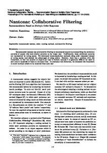
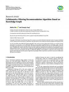
• P0’, P0n’, P0n2’ For all algorithms, we map predictions greater than +1 to +1 and predictions smaller than −1 to −1. We ran 1, 020 trials for each case. The results are shown in Figures 1 and 2. In all cases, the adapted algorithm yielded better predictions than the non-adapted variant. The mean average error decreased by 0.05 to 0.15 units depending on the algorithm, and the root mean squared error by 0.10 to 0.15 units. The relative accuracy gains on both corpora were different, suggesting that the prediction precision is dependent on the data used. For the MovieLens data, the best algorithm overall for both error measures was Pn2’, the adapted meanbased average weighted by the square of common ratings without default ratings. On the Jester data, the adapted mean algorithms yielded better results, but varying the other algorithm parameters did not change the error as much as with the MovieLens corpus. In general, errors were smaller on the Jester data than on the MovieLens data.

• Jester contains 617, 000 ratings of 100 jokes by 24, 900 users. Jester ratings range from −10 to +10 with a granularity of 0.01. The rating matrix is filled to about 25%. In order to compare the test results on both datasets, we ignored any of the additional movie information provided by MovieLens such as movie genres. The two error measures used are those described in [7]: • Mean average error (MAE): The mean difference between the rating and the prediction [13, 7]. • Root mean squared error (RMSE): The square root of the mean of squared differences between the ratings and the predictions [7]. Let (Ua(i) , Ib(i) ) be the user-item pair in test run i for i ∈ {1, . . . , n}, then the error measures are defined as: 1X |ra(i)b(i) − rã(i)b(i) | (8) MAE = n i s 1X RMSE = (ra(i)b(i) − rã(i)b(i) )2 (9) n i

7. Conclusion We proposed a modification to the class of memorybased collaborative rating prediction algorithms based on the Pearson correlation between users. The modification consists of adapting the ratings of other users using linear regression between user pairs before averaging them to calculate a prediction. We tested several variations of the basic algorithm all with and without the modification and found that

For both measures, smaller values indicate more accurate predictions. These errors are calculated on rating values scaled to the range [−1, +1]. Therefore predicting 0 in all cases would give MAEs and RMSEs not greater than 1. 1 http://movielens.umn.edu/ 2 http://www.ieor.berkeley.edu/∼goldberg/jester-data/

4

without adaptation (P) with adaptation (P’)

0.7

0.6 RMSE

0.6 MAE


0.7

0.5 0.4

0.5 0.4

0.3

0.3 P

Pn

Pn2

P0

P0n P0n2

P

Pn

Pn2

P0

P0n P0n2

Figure 1. MovieLens test results


0.7

0.6 RMSE

0.6 MAE


0.7

0.5 0.4

0.5 0.4

0.3

0.3 P

Pn

Pn2

P0

P0n P0n2

P

Figure 2. Jester test results

5

Pn

Pn2

P0

P0n P0n2

in all cases, the adaptation improved the prediction accuracy. The exact prediction accuracy however was found to be dependent on the dataset analyzed, suggesting additional tests are needed using other datasets. We showed that this modification does not affect the runtime complexity of the algorithm. In particular, this variation will be faster to calculate than other methods based on linear algebraic3 or probabilistic methods.

[6] J. L. Herlocker, J. A. Konstan, A. Borchers, and J. Riedl. An algorithmic framework for performing collaborative filtering. In SIGIR ’99: Proceedings of the 22nd annual international ACM SIGIR conference on Research and development in information retrieval, pages 230–237, New York, NY, USA, 1999. ACM Press. [7] J. L. Herlocker, J. A. Konstan, L. G. Terveen, and J. T. Riedl. Evaluating collaborative filtering recommender systems. ACM Trans. Inf. Syst., 22(1):5–53, 2004. [8] T. Hofmann. Collaborative filtering via gaussian probabilistic latent semantic analysis. In SIGIR ’03: Proceedings of the 26th annual international ACM SIGIR conference on Research and development in informaion retrieval, pages 259–266, New York, NY, USA, 2003. ACM Press. [9] H.-S. Huang and C.-N. Hsu. Smoothing of recommenders’ ratings for collaborative filtering. In Proceedings of the Fifth Conference on Artificial Intelligence and Applications (TAAI-2001), KaoHsiong, Taiwan, November 2001. [10] N. Kawamae and K. Takahashi. Information retrieval based on collaborative filtering with latent interest semantic map. In KDD ’05: Proceeding of the eleventh ACM SIGKDD international conference on Knowledge discovery in data mining, pages 618–623, New York, NY, USA, 2005. ACM Press. [11] D. Pennock, E. Horvitz, S. Lawrence, and C. L. Giles. Collaborative filtering by personality diagnosis: A hybrid memory- and model-based approach. In Proceedings of the 16th Conference on Uncertainty in Artificial Intelligence, UAI 2000, pages 473–480, Stanford, CA, 2000. [12] P. Resnick, N. Iacovou, M. Suchak, P. Bergstorm, and J. Riedl. GroupLens: An Open Architecture for Collaborative Filtering of Netnews. In Proceedings of ACM 1994 Conference on Computer Supported Cooperative Work, pages 175–186, Chapel Hill, North Carolina, 1994. ACM. [13] U. Shardanand and P. Maes. Social information filtering: Algorithms for automating “word of mouth”. In Proceedings of ACM CHI’95 Conference on Human Factors in Computing Systems, volume 1, pages 210– 217, 1995. [14] K. Yu, A. Schwaighofer, V. Tresp, X. Xu, and H.P. Kriegel. Probabilistic memory-based collaborative filtering. IEEE Transactions on Knowledge and Data Engineering, 16(1):56–69, 2004.

7.1. Future Work The following questions remain open and may guide future work on the topic: May it be useful to apply multiple linear regression on all other users’ ratings? This might increase accuracy, but also the runtime. It also remains to be seen whether a multiple linear regression approach might be mathematically related to other linear algebraic methods. On which datasets are the adapted ratings not an improvement? As proposed in Section 6, performing the tests with other datasets would be interesting. Unfortunately, not many rating datasets are available. Since many variations of the basic Pearson correlation-based algorithm exist [2, 3], a comparison with others of them would be possible.

References [1] J. Basilico and T. Hofmann. Unifying collaborative and content-based filtering. In ICML ’04: Proceedings of the twenty-first international conference on Machine learning, page 9, New York, NY, USA, 2004. ACM Press. [2] J. S. Breese, D. Heckerman, and C. Kadie. Empirical analysis of predictive algorithms for collaborative filtering. In Uncertainty in Artificial Intelligence. Proceedings of the Fourteenth Conference, pages 43–52. Morgan Kaufmann Publishers, 1998. [3] Y. Chuan, X. Jieping, and D. Xiaoyong. Recommendation algorithm combining the user-based classified regression and the item-based filtering. In ICEC ’06: Proceedings of the 8th international conference on Electronic commerce, pages 574–578, New York, NY, USA, 2006. ACM Press. [4] M. Connor and J. Herlocker. Clustering items for collaborative filtering, 2001. [5] K. Goldberg, T. Roeder, D. Gupta, and C. Perkins. Eigentaste: A constant time collaborative filtering algorithm. Inf. Retr., 4(2):133–151, 2001. 3 While linear regression uses tools from linear algebra, it does not involve the quadratic (or higher) complexity associated with problems such as SVD decomposition or matrix inversion.

6