Adaptive Hierarchical Incremental Grid Growing: An architecture for high-dimensional data visualization. Dieter Merkl1,2, Shao Hui He3, Michael Dittenbach2, ...
Adaptive Hierarchical Incremental Grid Growing: An architecture for high-dimensional data visualization Dieter Merkl1,2 , Shao Hui He3 , Michael Dittenbach2 , and Andreas Rauber3 1
3
Institut f¨ ur Rechnergest¨ utzte Automation, Technische Universit¨at Wien http://www.rise.tuwien.ac.at/ 2 Electronic Commerce Competence Center–EC3, Wien http://www.ec3.at/ Institut f¨ ur Softwaretechnik und Interaktive Systeme, Technische Universit¨at Wien http://www.ifs.tuwien.ac.at/ Keywords: Hierarchical clustering, adaptive architecture, text mining
Abstract— Based on the principles of the selforganizing map, we have designed a novel neural network model with a highly adaptive hierarchically structured architecture, the adaptive hierarchical incremental grid growing. This feature allows it to capture the unknown data topology in terms of hierarchical relationships and cluster structures in a highly accurate way. In particular, unevenly distributed real-world data is represented in a suitable network structure according to its specific requirements during the unsupervised training process. The resulting three-dimensional arrangement of mutually independent maps reveals a precise view of the inherent topology of the data set.
1
Introduction
The self-organizing map (SOM) [9] is an artificial neural network model that proved to be exceptionally successful for data visualization applications where the mapping from an usually very high-dimensional data space into a two-dimensional representation space is required. The remarkable benefit of SOMs in this kind of applications is that the similarity between the input data as measured in the input data space is preserved as faithfully as possible within the representation space. Thus, the similarity of the input data is mirrored to a very large extend in terms of geographical vicinity within the representation space. However, some difficulties in SOM utilization remained largely untouched despite the huge number of research reports on applications of the SOM. First, the SOM uses a fixed network architecture in terms of number and arrangement of neural processing elements which has to be defined prior to training. Obviously, in case of largely unknown input data characteristics it remains far from trivial to determine the network architecture that allows for satisfying results. Thus, it certainly is worth considering neural network models that determine the number and arrangement of units during their unsupervised training process. We refer
to [1, 2, 7, 8] for recently proposed models that are based on the SOM, yet allow for adaptation of the network architecture during training. Second, hierarchical relations between the input data are not mirrored in a straight-forward manner. Such relations are rather shown in the same representation space and are thus hard to identify. Hierarchical relations, however, may be observed in a wide spectrum of application domains, thus their proper identification remains a highly important data mining task that cannot be addressed conveniently within the framework of the SOM. The hierarchical feature map (HFM) as proposed in [13], i.e. a neural network model with hierarchical structure composed from independent SOMs, is capable of representing the hierarchical relations between the input data. In this model, however, the sizes of the various SOMs that build the hierarchy as well as the depth of the hierarchy have to be defined prior to training. Thus, considerable insight into the structure of the input data is necessary to obtain satisfying results. Only recently, we have proposed the growing hierarchical self-organizing map (GHSOM) as an artificial neural network architecture designed to address both limitations within a uniform framework [4, 5, 6]. Similar to the HFM, a hierarchical layout of the architecture is chosen. In case of the GHSOM, however, this hierarchical layout is determined during the unsupervised training process guided by the peculiarities of the input data. In this work, we describe an alternative model, the adaptive hierarchical incremental grid growing (AHIGG), where the individual layers of the hierarchical architecture are variants of the incemental grid growing (IGG) network as originally proposed in [2, 3]. The major difference of the AHIGG as compared to the GHSOM is that maps on individual layers may grow irregularly in shape and may remove connections between neighboring units. In this way a better understanding of the underlying input data can be gained which lends itself for easy visual exploration. The remainder of this paper is organized as follows.
293
Section 2 contains a brief review of the incremental grid growing neural network, an adapted version of which will be used as building blocks for the AHIGG. In Section 3 we provide an outline of architecture and training process of the AHIGG. Section 4 contains the description of an application scenario for the AHIGG, namely the organization of document archives. Finally, we present our conclusions in Section 5.
new1 error node
(a)
new2
(b)
new1
2
error node
A quick review of Incremental Grid Growing
The incremental grid growing (IGG) model as proposed in [2, 3] combines the topology preserving nature of SOMs with a flexible and adaptive architecture that represents cluster structures during an unsupervised training process. Initially, the IGG network consists of four connected units, each of which is assigned an initially random weight vector of the same feature space as the training data. During the training process, the network is dynamically changing its structure and its connectivity to resemble the topology of the input data. The training process consists of a sequence of iterations where each cycle consists of the following three phases: (1) The SOM training phase: The SOM algorithm is applied to train the current map. The weight vectors of the units are adapted to the highdimensional relations in the input data. (2) The expansion phase: New units are added to that region at the perimeter of the current map that are responsible for the largest quantization error. (3) The adaptation of connections phase: Connections between neighboring units are added or removed from the network depending on the metric distance between the units’ weight vectors. Thus, cluster boundaries and discontinuities in the input data become explicitly visible.
new3
(c)
X
(xk − mik )2
(d)
Figure 1: IGG–Expansion phase
expansion phase new units are generated at the unoccupied neighboring grid positions of the error node, as symbolized in Figures 1(b) and 1(d). Finally, during the adaptation of connections phase the metric distance of weight vectors at neighboring grid positions are analyzed. A connection between the respective units is established if the distance of their weight vectors is below a particular treshold value τconnect , as symbolized in Figures 2(a) and 2(b). However, if this distance is larger than a second threshold parameter τdisconnect then a possible existing connection between the units is removed, as symbolized in Figures 2(c) and 2(d). The thus established connections play a critical role during the then following next SOM training phase because only connected nodes in the neighborhood of the winner are adapted.
weight vectors close
A note on the three phases is in order. During the SOM training phase the quantization error of the various units is cumulated as detailed in Eq. (1) with i being the index of the unit in question, mi that unit’s weight vector, x an input vector, and t referring to the current SOM training iteration. Ei (t + 1) = Ei (t) +
new2
(a)
(b)
weight vectors distant
(1)
k
(c)
After a fixed number of SOM training iterations the unit with the largest cumulated quantization error is selected as the error unit, as symbolized in Figures 1(a) and 1(c). When given a rectangular network layout, each unit may have four neighbors. During the
(d)
Figure 2: IGG–Adaptation of connections phase
294
3
A hierarchically growing IGG network
Basically, the AHIGG is composed of a hierarchical arrangement of independent IGG networks on each of its layers. Each layer is resposible for input data representation at a specific level of granularity. Pragmatically speaking, a rough idea of the similarities in the input data is represented in the first layer of the AHIGG. Each unit of this first layer map may be expanded to an individual map on the second layer of the hierarchy if the desired level of granularity in data representation is not reached yet. Thus, the layers further down the hierarchy give a more detailed picture of subsets of the input data. Consider Figure 3 as a simple pictorial representation of an AHIGG consisting of three layers. layer 1
layer 2
layer 3
Please note this initialization scheme is different to the one proposed originally for the IGG network in [2]. We have chosen this scheme because it allows for weight vectors being roughly aligned within the input data space. After initialization, the network is training according the the SOM algorithm for a fixed number λ of input vector presentations. Then, the border unit with the largest mean quantization error is selected and new neighboring units are added to the network. Finally, the weight vectors of neighboring units are checked for possible adaptation of connections. This training process follows the description as given in Section 2. This training process is repeated until the mean quantization error of the map falls below a certain fraction τ1 , 0 < τ1 < 1, of the mean quantization error of it’s parent unit. A fine-tuning phase is then performed where only the winner is adapted and no further units are added to the network. After this fine-tuning phase, each unit is checked for possible hierarchical expansion. More precisely, the mean quantization error of each unit is computed and units with too high a mean quantization error are expanded on the next layer of the hierarchy, i.e. for those units a new map on the next layer of the hierarchy is established. The mean quantization error of a units is compared to the mean quantization error of the unit at layer 0 and a simple threshold logic is used for the decision of hierarchical expansion. Each unit for which Eq. (4) holds true is further expanded. In this formular, τ2 represents the threshold, 0 < τ2 < 1. mqei > τ2 · mqe0
Figure 3: Architecture of the AHIGG At the beginning of training the weight vector of a single unit map at layer 0 is initialized as the statistical mean of the input data. The mean quantization error of this unit as given in Eq. (2) will play a crucial role during the training process of the AHIGG. In this formula, I refers to the set of input data, n is the cardinal number of I, x is an input data, and m0 is the weight vector of the single unit at layer 0. mqe0 =
1X ||m0 − x|| n
(2)
x∈I
In the next step of training, a map at layer 1 is created that consists of a small number of units, e.g. four units arranged in a square. The weight vectors of these units are initialized randomly but taking into account the weight vector of its ‘parent’ unit in the preceding layer (mparent ) together with the mean quantization error of that unit (mqeparent ). The initialization scheme is given in Eq. (3), with vrand denoting a random vector of length 1. mi = mparent + mqeparent · vrand
(3)
(4)
A difference to the original IGG model can be found in the initialization of weight vectors of newly added units. In [2] an intialization strategy is proposed the preserves the local topology by taking into account statistical means. More precisely, the new weight vectors are initialized such that the error node’s weight vector is the statistical mean of its neighbors. Apart from the fact that in some cases the new weight vectors may lie beyond the data space, this scheme may produce isolated units at the perimeter of the map. The reason for this phenomenon is explained by the location of the growth process. We believe that a topology preserving initialization works well in the interior of the map where the extent of the interpolation is given by the enclosure. Such a strategy can be found for example in the growing grid network [8]. However, steady continuation into the open area at the perimeter of the IGG may be fatal. In the most pathological case, the connections to the new units are immediately removed after each growing step. They thus become isolated and are not likely to contribute to the share of input patterns. We therefore suggest to initialize the new weight vectors randomly with a vector from the �-environment of the error node, as given in Eq. (5).
295
In this formular, mnew refers to the weight vector of a newly added unit, merror is the weight vector of the error unit, vrand is a random vector of length 1, and � is a small constant, i.e. 0 < �