Adaptive Resource Allocation Scheme for 2-hop Non-regenerative MIMO Relaying System Zhang Qi, Wang Ying, Zhang Ping Wireless Tech. Innovation Lab., P.O.Box 92 Beijing University of Posts and Telecommunications, Beijing, China No.10, Xi Tu Cheng Road
[email protected] mode. For the regenerative mode, the relaying nodes need to know about each other’s existence [7], which may require much signaling exchange between the relaying nodes to be able to execute decoding and recoding; therefore, the optimal PA scheme for the non-regenerative mode is the main concern in this paper, which is considered to be a more practical mode in real system.
Abstract-Resource allocation scheme for traditional MIMO system have been widely studied by the researchers. However, when MIMO technique is applied into the relaying system, where several separated terminals form a virtual receive array (VAA) and relay the signal from the transmitter to the receiver, the aforementioned issues which have close relationship with the system performance should be solved before MIMO relaying system is deployed on a large scale. In this paper, the channel capacity for 2-hop MIMO relaying system is derived from the perspective of information theory. Optimal resource allocation under aggregate power constraint between relaying nodes in closed form is proposed for the case with two relaying nodes. Numerical results indicate that MIMO relaying system will achieve higher channel capacity than traditional MIMO does and the positions of the relaying nodes affect the system performance directly. Keywords-resource allocation, allocation, MIMO relaying
channel
capacity,
In section II, a model for 2-hop non-regenerative MIMO relaying system is developed. In section III, the expression of channel capacity for this model is derived in detail, and the optimal resource allocation, or PA scheme, under aggregate power constraint maximizing the channel capacity is presented. In section IV, some numerical results are provided to show the performance of the algorithm. Finally, some useful conclusions are drawn on the power allocation scheme in section V.
power
II. I.
INTRODUCTION
In the radio propagation environment, there may be some “blind zones” caused by surrounding buildings. To combat deep fading in these areas, cooperative relaying is proposed [1], in which several terminals serve as intermediate nodes to forward the signals, provide spatial diversity and save transmit power of the transmitter. Generally speaking, cooperative relaying can be divided into two modes: regenerative relaying and non-regenerative relaying. In the regenerative mode, the transmitted signals are decoded and re-encoded at the relaying nodes, and then forwarded to the receiver. While in the non-regenerative mode, the signals are simply amplified at the relaying nodes and forwarded to the receiver. There are two main areas in recent research about cooperative relaying system, one is based on repeater [2][4]; however, the more interesting area about cooperative relaying is based on a promising antenna technology, multiple-input multiple-output (MIMO), which is thought as a competitive candidate in 4G system. Although there has been much work [5]-[8] on capacity analysis and power allocation (PA) scheme for MIMO relaying system, and some heuristic schemes have been developed, no optimal PA scheme has been proposed in closed form even for the simple case with two relaying nodes in the non-regenerative
SYSTEM MODEL
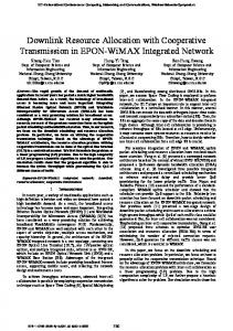
Figure 1 displays the MIMO relaying system model used in this paper. In this model, the transmitter has t transmit antennas, and the relaying nodes include r terminals while each only has one antenna, forming a virtual receive antenna
A N
H1
S1
S2
S
R2
. .
. . . St
Transmitter
Power Allocation
R1
HD
R
H2
Channel Estimation
D r-1
ND W
Rr
Relaying Nodes
Receiver
Figure 1: System Model for 2-hop non-regenerative MIMO Relaying
1
This research is supported in part by NSFC, project No. 60302024 and high-tech cooperation project between Chinese and Swedish government and Ericsson Company.
IEEE Communications Society / WCNC 2005
995
0-7803-8966-2/05/$20.00 © 2005 IEEE
array, the receiver has only 1 antenna. The transmitter sends the signal vector X, and the relayed signal vector R contains the signal component received by each relaying node, such that the first hop between the transmitter and all the relaying nodes is the traditional MIMO channel, which is characterized by channel matrix H1. After being amplified and forwarded, the received signal at the receiver is given by
Y = H2AR+ W = H2A(H1X + N) + W = HX+ N'
III.
CAPACITY ANALYSIS AND POWER ALLOCATION SCHEME
In the case that the channel state information (CSI) is not known at the transmitter, the covariance matrix of the input signal X has the diagonal form with equal diagonal elements to maximize the channel capacity of the first hop [9], then the corresponding covariance matrix of the input signal X is
(1)
QX =
in equation (1), g11 h11(1) ... g11 h1(t1) g11 h11(1) ...h1(t1) H1 = ... ... = ⋅ ... = G1H1 ' (1) (1) (1) (1) g1r hr1 ...hrt g1r hr1 ... g1r hrt g 21 h21 g 21 H2 = ... ... = g 2 r h2 r
(2)
where P0 is the transmitted signal power, and I t is the torder identity matrix. Based on the classical Shannon theory, channel capacity is the maximal average mutual information between input symbol and output symbol. Note that in the following derivation, the direct path from the transmitter to the receiver is not taken into account. Since HX and N ' are uncorrelated (Appendix A), the channel capacity for every implementation of the channel is then given by [9]
h21 ⋅ ... = G 2H 2 ' h2 r g 2r
a1 and A = ... a r
C = I [X; (Y, H )] = I [X; Y | H ] = H (Y ) − H (N') = log(det[πeQ Y ]) − log(det[πeQ N' ])
(3)
where H (⋅) is the entropy of a random vector.
where Gi and Hi ' are the path loss and the fast fading for ith hop respectively. Orthogonal transmission is adopted for the 2nd hop, so H2 is diagonal. Assuming that the entries of all fading matrixes, i.e. H1' and H2 ' , are independent complex Gaussian distributed variables with independent real and imaginary parts each with variance 1/2 in the proposed model. A is diagonal and the diagonal elements of A denote the amplifying factor for each relaying node. In addition, the received signals at the relaying nodes and the receiver are corrupted by additive Gaussian noise, N and W, which are zero-mean complex Gaussian noise with independent real and imaginary parts each with variance σN2 /2 and σw2 /2. In (1),
In equation (3), QY is the covariance matrix of the received signal, and QN’ is the covariance matrix of the equivalent noise.
[
]
Q Y = E YY H = HQ X H H + Q N '
[
Q N ' = E N'N'
H
] = σ H AA H 2 N
H
2
σ N2 h21 2 g 21a12 + σ w2 =
H and N ' are the equivalent channel matrix and noise. Noted that the above description does not include the direct path the transmitter and the receiver, which are represented by the gray dotted lines and HD and ND. HD is the channel matrix of direct path, including path loss and fast fading, and ND is the noise of direct path, which has the same distribution function as N or W with variance σD2. The case with direct path and without direct path will be discussed respectively in detail in section III.
H 2
(4.1)
+ σ w2 Ir
(4.2) ... 2 2 2 2 σ N h2 r g 2 r ar + σ w
where E[⋅] is the expectation of random variable. To limit the energy consumption in the system, the aggregate power constraint is put on the transmit power of relaying nodes. In other words, the sum of the transmit power of relaying nodes should not exceed a predefined threshold P. The transmitted signal vector V by relaying nodes could be extracted from equation (1),
Assuming that the channel estimation module could estimate channel matrix H1 and H2 (and HD) perfectly, the channel matrix H1 and H2 (and HD) are then fed into the power allocation module. The output of the PA module is the diagonal elements of A, i.e. the amplifying factors. These diagonal elements are sent to the corresponding relaying nodes via additional feedback channel and used to amplify the signals received by the relaying nodes.
IEEE Communications Society / WCNC 2005
P0 It t
996
V = AR = A(H1X + N)
(5.1)
then the covariance matrix of V is
0-7803-8966-2/05/$20.00 © 2005 IEEE
[
Q V = E AR (AR )
H
[
]
(
) ]
= E A (H 1 X + N ) X H + N A H
N 1
H
H
H P = 0 AG 1H '1H 1' G 1 A H + σ N2 AA H t Η Pg = 0 1 ΑΗ 1' Η1' Α Η + σ N2 AA H t
2 P1 g 21g11 h21 2 2 2 P σ N P1 g 21 h21 + PR1 σ w C = log detI 2 + 0 2 2 P2 g 22 g12 h22 2 σ N2 P2 g 22 h22 + PR2 σ w2
(5.2)
f1 (P1 ) ' ' H H1 H1 = log detI 2 + f P ( ) 2 2 = log[(H11H 22 − H12 H 21 ) f1 (P1 ) f 2 (P − P1 ) + H11 f1 (P1 ) + H 22 f 2 (P − P1 ) + 1]
The aggregate power constraint of relaying nodes could be express by the trace of Qv Pg t (1) 2 + σ N2 trace(Q V ) = ∑ a 0 1i ∑ hij i =1 t j =1 r
r
= ∑a P i =1
= log[ f (P1 )]
2 i
2 i Ri
r
= ∑ Pi ≤ P
fi (Pi ) =
0 ≤ Pi ≤ P
HH
)
=
αi Pi
i = 1,2
βi Pi + γ i
'H 1
0≤P1 ≤P
Since H H is non-negative definite, then
[
∆ 1 = H 11 H 22 − H 12 H 21 = det H '1 H 1'
−1 N'
t
H
]≥ 0 , and
∆ i = H ii = ∑ hij ≥ 0, i = 2,3 .
−1 N'
P = log detIr + 0 HHHQN−1' t
2
j =1
It is easy to find that f (P1) is concave function within 0 ≤ P1 ≤ P through taking the second order derivative with respect to P1 . The problem is to find the optimal P1 to maximize C, i.e., maximize f (P1) . Applying convex function theory, the optimal power allocation scheme could be obtained in closed form.
P = log detIt + 0 HHQN−1' H t P = log detIt + 0 H1H AH HH2QN−1' H2 AH1 t 2 P1g21g11 h21 2 σ N2 P1g21 h21 + PR1 σ w2 P = log detIr + 0 ... t 2 Pr g2r g1r h2r 2 σ N2 Pr g2r h2r + PRr σ w2
h11(1) h12(1) ⋅ ⋅ ⋅ h1t (1) h11(1) h12(1) ⋅ ⋅ ⋅ h1t (1) H H = 11 12 = (1) (1) H H h h ⋅ ⋅ ⋅ h (1) h (1) h (1) ⋅ ⋅ ⋅ h (1) 21 22 2t 21 22 2t 21 22
' 1
( [ ]) [ ]) = log(det[HQ H + Q ] ⋅ det[Q ]) = log(det[I + HQ H Q ]) X
2 σ P g2i h2i + PRi σ
2 w
=∆1 f1(P1) f2(P−P1) +∆2 f1(P1) +∆3 f2(P−P1) +1
C = log det HQX HH + QN' − log(det QN'
r
2
2 N i
f (P1) =(H11H22 −H12H21) f1(P1) f2(P−P1) +H11f1(P1) +H22f2(P−P1) +1
Substituting (4.1) and (4.2) into (3), then the channel capacity could be expressed as
H
2
and
node.
N'
(
P0 Pi g2i g1i h2i
H
'H 1
' 1
where PR (i = 1, 2 ...r ) is the received power (including the i received signal power and the noise power) at each relaying node, Pi (i = 1,2...r ) is the transmit power of each relaying
H
(7)
where
(5.3)
i =1
X
' ' H H 1 H 1
' ' H H1H1
(6)
[
]
df ' ' ' ' = ∆1 f1 (P1 ) f 2 (P − P1 ) + f1 (P1 ) f 2 (P − P1 ) + ∆2 f1 (P1 ) + ∆3 f 2 (P − P1 ) (8) dP1 2
= K1P1 + K2 P1 + K3 = 0
0 ≤ P1 ≤ P
where K1 = ∆1α1α 2 (γ 1β 2 − γ 2 β1 ) + ∆ 2α1γ 1β 2 − ∆ 3α 2γ 2 β1 2
Note that the determinant identity det[I + XY] = det[I + YX] is applied into the above derivation. Since the receiver knows the CSI, the channel capacity for every implementation of channel can be maximized, and then the average channel capacity is maximized naturally.
2
K 2 = −2γ 1 [∆1α1α 2 (γ 2 + β 2 P ) + ∆ 2α1β 2 (γ 2 + β 2 P ) + ∆ 3α 2γ 2 β1 ]
[
K 3 = γ 1 ∆1α1α 2 P(γ 2 + β 2 P ) + ∆ 2α1 (γ 2 + β 2 P ) − ∆ 3α 2γ 2γ 1 2
]
then the optimal P1 maximizing f (P1) (or C) is
For the case with two relaying nodes, substituting r = 2 into (6)
2
P1 =
− K 2 ± K 2 − 4 K1K3
(9)
2 K1
Choosing the P1 that satisfies 0 ≤ P1 ≤ P as the optimal solution. If both P1 are greater than P or less than zero, then
IEEE Communications Society / WCNC 2005
997
0-7803-8966-2/05/$20.00 © 2005 IEEE
method could be used to find the optimal resource allocation scheme. As displayed in Fig 1, the received signal Y consists of two parts, the relayed signal YR and the direct signal YD, Y is then given by
comparing the channel capacity at the boundary points, P1 = P and P1 = 0 , and selecting the better one. In this case, the total power is allocated to one of the two relaying nodes. In the above analysis and derivation, direct path is not taken into account. For the case with the direct path, the similar
YR H 2 A (H 1 X + N ) + W H 2 AH 1 H 2 AN + W ' Y= = = H X + N = = HX + N + Y H X N D D D D D
(10)
where H is the equivalent channel matrix and N' the equivalent noise. The channel capacity is
( )
C = H (Y ) − H (Y | X ) = H (Y ) − H N '
2 P1 g 21 g11 h21 2 2 2 σ N P1 g 21 h21 + PR1σ w P ... = log (det [Γ ]) + log det I r + 0 t 2 Pr g 2 r g1r h2 r 2 σ N2 Pr g 2 r h2 r + PRr σ w2
where
Γ = It +
P0 tσ D
H
2
HD HD
' −1 ' H H1Γ H 1
(11)
, which is Hermitian and positive definite, so the inverse of Г always exists. Obviously, Г is the
additional term resulted by the direct path. For the case with two relaying node, substituting r = 2 into (11), since Г is deterministic, the channel capacity C could be maximized by the similar method used in (7). NUMERICAL RESULTS Channel Capacity(bits/transmission)
IV.
In this section, some numerical results are provided to show the performance of the optimal PA scheme. In the simulations the 2 relaying nodes are assumed close to each other. The transmitter is located at (0,0), and the receiver at (100,0), the two relaying nodes may be at any location within the study area. The transmitter power is fixed to be 20w. The noise power at relaying nodes and receiver are 2.5×10⁻¹⁰w, and the path loss factor is 4. In fig 2 and fig 3, the horizontal axes represent the position of the relaying nodes, and the vertical axis represents the corresponding average channel capacity in bits/transmission. Fast fading is taken into consideration, while shadowing is not taken into account. Fig 2 shows the performance comparison between the relaying transmission with the optimal PA (OPA) scheme and the direct transmission, in which the horizontal plane is the channel capacity for the direct transmission, and the convex surfaces stand for the channel capacity for the relaying transmission with and without direct path. In fig 2, the red surface is the channel capacity for relaying transmission with direct path, and the blue surface is for the relaying transmission without direct path. It can be observed that in the most of the study area, the performance of the relaying transmission without direct path is better than that of the direct transmission. We define the area where the relaying transmission could bring performance gain as
IEEE Communications Society / WCNC 2005
25
OPA with direct path OPA without direct path, Direct Transmission
20
15
10
5 50
R e ce i ve r
0 y(m)
Tra n s m i tte r
-50
-50
0
50
100 x(m)
150
Figure 2: Performance comparison between the relaying transmissions with OPA and direct transmission, Power Constraint: 10 watt
effective area. The performance of the relaying transmission deteriorates when the relaying nodes is out of the effective area, in this case, network should employ the direct transmission only. This could be a guidance when to start relaying mechanism in the network. However, for the case with direct path, the system performance with OPA is always better than direct transmission in the simulation area,
998
0-7803-8966-2/05/$20.00 © 2005 IEEE
Channel Capacity (bits/transmission)
20
nodes depends on the power constraint. With the increase of the constraint power, the position moves towards the transmitter.
Power Con. = 10 watt Power Con. = 0.1 watt Power Con. = 0.001 watt Direct Transmission
V. 15
Channel capacity and power allocation scheme are important issues in the research of MIMO system. For the traditional MIMO system, the achievable channel capacity is well derived from the perspective of information theory. Based on the channel capacity, the PA scheme could be obtained directly. For MIMO relaying system, however, more problems need to be considered, such as the PA between the relaying nodes and the geographic distribution of those nodes. This paper investigates a 2-hop MIMO relaying system, wherein the first relaying channel composes of a traditional MIMO channel (as indicated in equation (1)). Assuming the CSI is not known at the transmitter but known at the receiver, the channel capacity expression and the optimal PA scheme with and without direct path to achieve the maximal channel capacity are derived in closed form for the case with 2 relaying nodes. Numerical results indicate that the use of relaying transmission may greatly increase the achievable rate on fading channel if the CSI can be estimated perfectly at the receiver, while the gain heavily depends on the relaying power constraint. In addition, to achieve the best system performance, the relaying nodes should be sited (for the fixed relaying nodes) at the proper positions. For the case without direct path, if the position of the relaying nodes is out of effective area, the system performance will be deteriorated. While for the case with direct path, the performance of relaying system is always better than that of the direct transmission system.
10
5
0 -40
-20
0
20
40
60
80
100
120
140
x(m)
Channel Capacity (bits/transmission)
Figure3: Average channel capacity under different power constraints-without direct path: 10 watt, 0.1 watt and 0.001 watt
20
Power Con. = 10 watt Power Con. = 0.1 watt Power Con. = 0.001 watt Direct Transmission
15
10
5
0 -40
-20
0
20
40
60
80
100
120
CONCLUSIONS
140
x(m)
ACKNOWLEDGEMENT
Figure4: Average channel capacity under different power constraints-with direct path: 10 watt, 0.1 watt and 0.001 watt
The authors of this paper thank Hu Rong, Zhang Zhang, and Peter Larsson for their helpful discussions and suggestions, valuable comments. Their support is gratefully acknowledged. The authors also thank the other members for many useful interactions and for contributing their broad perspective in refining the ideas in this paper.
which is an inevitable and reasonable result because the relaying system introduces the additional power. The performance difference between OPA with and without direct path can also be seen in Fig 3 and Fig 4. Fig 3 shows that the position where the relaying nodes provide the maximal channel capacity is between the transmitter and the receiver. With the increase of the constraint power, the position moves towards the transmitter. This is useful to perform relaying selection (or siting) under specific power constraint. Besides, It can be seen that the size of the effective area also depends on the power constraint for the relaying nodes. With the increase of the power constraint, the effective area expands. However, fig 4 shows that OPA with direct path always bring performance in all power constraints: 10watt, 0.1watt and 0.001watt. Similar with the case without direct path, the best position of the relaying
IEEE Communications Society / WCNC 2005
APPENDIX A Rewriting equation (1) here Y = H2 AR + W = H2 A(H1 X + N) + W = HX + N'
(A.1)
To apply the mutual information formulation, HX and N’ should be uncorrelated.
999
0-7803-8966-2/05/$20.00 © 2005 IEEE
HX = H 2 AH1 X (1) (1) a1 g 21 h21 g11 h1t g11 h11 ... ... ... = (1) (1) a g 2r h2 r g1r hrt r g1r hr1 g 21g11 h21a1 h11(1) x1 + ... + h1t (1) xt ... = g g h a h (1) x + ... + h (1) x rt t 2r 1r 2 r r r1 1
(
)
(
)
g 21 h21a1n1 + w1 N' = H 2 AN + W = ... g h a n +w r 21 2 r r r
(A.2) x1 ... xt
(A.3)
[7] Mischa Dohler, Athanasios Gkelias, Hamid Aghvami, “A Resource Allocation Strategy for Distributed MIMO Multi-Hop Communication Systems,” IEEE COMMUNICATIONS LETTERS, VOL. 8, NO. 2, FEBRUARY 2004 [8] Peter Larsson, “Large-Scale Cooperative Relay Network with Optimal Coherent Combining under Aggregate Relay Power Constraints,” Future Telecommunications Conference, 2003, Beijing. [9] E. Telatar, “Capacity of multi-antenna Gaussian channels,” Eur. Trans.Telecommun., vol. 10, no. 6, pp. 585–595, Nov./Dec. 1999.
The cross correlation matrix is between HX and N ' is given by
[
R(HX)N' = E (HX)N'H
]
(
)
(
)
g g h a h (1) x + ...+ h (1) x 1t t 21 11 21 1 11 1 ... = E (1) (1) g2r g1r h2r ar hr1 x1 + ...+ hrt xt
⋅
g21h21a1n1 + w1 ... g2r h2r ar nr + wr
H
=O (A.4) From (A.4), it could be found that HX and N ' are uncorrelated, or independent since they are Gaussian distributed random vector. REFERENCES [1] J. Nicholas Laneman, “Cooperative Diversity in Wireless Networks: Algorithms and Architectures,” M.I.T. Doctoral Dissertation, Sep.2002 [2] Zhang Qi, Zhang Jingmei, Shao Chunju, Wang Ying, Hu Rong, Zhang Ping, “Power allocation for Regenerative Relay Channel with Rayleigh Fading,” IEEE VTC 2004 spring [3] Zhang Jingmei, Zhang Qi, Shao Chunju, Wang Ying, Zhang Zhang, Zhang Ping, “Adaptive Optimal Transmit Power Allocation for Two-hop Non-regenerative Wireless Relaying System,” IEEE VTC 2004 spring [4] Zafer Sahinoglu, Philip Orlik, “Regererator Versus Simple-Relay With Optimum Transmit Power Control for Error Propagation,” IEEE Communications letters, Vol.7, No.9, Sep.2003 [5] M.Dohler, E.Lefranc, H.Aghvami, “Virtual Antenna Arrays for Future Wireless Mobile Communication Systems,” ICT 2002, June 2002 [6] M. Dohler, A. Gkelias, H. Aghvami, “2-hop distributed MIMO communication system,” ELECTRONICS LETTERS 4th September 2003 Vol. 39 No. 18
IEEE Communications Society / WCNC 2005
1000
0-7803-8966-2/05/$20.00 © 2005 IEEE