A great deal of photolithographic activity in recent years has been centered on thick photoresist films. Thin film heads (TFH), micromachining and sensor ...
SPIE 1997 3049-72
Advanced Simulation Techniques for Thick Photoresist Lithography Warren W. Flack, Gary Newman Ultratech Stepper, Inc. San Jose, CA 95134
D. Bernard, J. Rey, Y. Granik, V. Boksha Technology Modeling Associates Sunnyvale, CA 94086
A great deal of photolithographic activity in recent years has been centered on thick photoresist films. Thin film heads (TFH), micromachining and sensor fabrication are examples of applications requiring this type of processing. The needs of the TFH industry are currently the technology driver for thick photoresist processing. Modern TFH manufacturing processes require 1 µm resolution in layers ranging in thickness from 5 to as much as 25 µm. These large aspect ratios not only make the lithographic process difficult, but add complexity to the evaluation and measurement of experimental wafers. This is particularly true for the large number of measurements needed for process optimization and control. Well-calibrated and easy to use modeling techniques for analysis of the impact of optical system design and photoresist process changes would be extremely valuable for process lithography engineers. The photoresist development process involves complex dissolution and polymer chemistry. It forces simulator developers to implement empirical models with definitions and assumptions that only indirectly reflect the underlying physical and chemical processes. However, with appropriate calibration such an approach provides results with accuracy better than 90% at reasonable computational time for any given combination of a particular photoresist base material, photoactive component, development and bake conditions. A method has been developed that allows accurate simulation of pattern profiles in photoresist in excess of 10 µm thick. The method uses the DEPICT® photolithography simulator to model i-line exposure, bake and development of Shipley SJR5740 thick film photoresists with an Ultratech 2244i Wafer Stepper®. Kim model inputs were estimated from a family of development rate curves obtained by processing wafers with a range of expose energies for logarithmically increasing develop times and measuring thickness change as the develop process occurred. These results were compared with dissolution results obtained using a laser-based dissolution rate monitor. Uncertainties in the measured photoresist absorbence, photosensitivity and refractive index coefficients were estimated and their influence on the simulated results were considered. An optimization
Flack, Newman, Bernard et.al.
1
SPIE 1997 3049-72
procedure and algorithm that allows quantitative comparison of experimental and simulated photoresist profiles is presented. Simulated photoresist profiles were compared with patterns obtained from processed wafers. As a further test of the models, pattern profiles were simulated for 2 µm spaces in 10 µm thick photoresist through focus. Experimental and simulated pattern profiles from a range of exposure doses were also compared. Key Words: photoresist simulation, thick photoresist, submicron 1X steppers, thin film heads
1.0 INTRODUCTION Photoresist films for semiconductor industry applications are typically less than 2 µm thick for critical pattern transfer operations such as dry etching and high energy implants. However, there are an increasing number of applications for thicker photoresist films in the 5 to 25 µm range. When compared to thin photoresist films, the lithography for these thick photoresist films provides a new set of challenges for process optimization. An example of a thick photoresist application is the fabrication of thin film heads (TFH) for disk drive storage systems [1]. Overall data storage and drive speed is closely related to the track width of the TFH. As drive performance has increased, minimum critical dimensions (CDs) have continued to decrease and are approaching 1 µm. However, the large topography present in the typical TFH requires the use of photoresist films of approximately 10 µm thickness. This results in a loss of CD control due to variations in photoresist thickness in excess of 50% in regions adjacent to large topography [2]. Slopes in the thick photoresist film also reduce the CD control. There are further detrimental effects on CD control from the specific photoresist optical properties and develop characteristics. First, the bulk absorption effect of the photoresist reduces the effective dose at the bottom of the film. This effect is further impacted by the wet development process which produce sloped profiles [2]. Another effect which impacts CD control are highly reflective metal films, which can result in standing wave phenomena. Consequently, the properties of a thick photoresist film will have a dramatic impact on CD control and process latitude. The extremely large aspect ratios required for TFH manufacturing add complexity to the evaluation and optimization of lithographic processes. Optical inspection techniques are inadequate for this job. Cross-sectional SEM techniques provide the necessary information, but at substantial cost and long evaluation times. The extensive SEM support, combined with the large number of measurements required for characterization of new lithographic process, make working with thick films a daunting task. The semiconductor industry has made extensive use of lithography process modeling to reduce the development time for process optimization and to obtain a better understanding of complex problems. For example, i-line lithography and deep UV excimer lithography have been
Flack, Newman, Bernard et.al.
2
SPIE 1997 3049-72
successfully modeled using a number of commercially available simulation packages. Several studies have been performed for thick photoresist simulation [3, 4]. However, most of this work involved 4 µm minimum CDs using older g-line photoresist materials. More advanced processes, with smaller CDs and i-line photoresists, could clearly benefit from process modeling. Well-calibrated and easy to use modeling techniques for analysis of the impact of optical system design and photoresist process changes would be extremely valuable for process lithography engineers. The purpose of this work is to simulate a 2 µm CD process in 10 µm of Shipley SJR5740 photoresist and compare the model results to experimental data obtain using an Ultratech 2244i Wafer Stepper.
2.0 EXPERIMENTAL METHODS 2.1 Lithography Equipment All lithography was performed on an Ultratech Stepper 2244i Wafer Stepper lithography system. The Ultratech stepper is based on the 1X Wynne-Dyson lens design employing broadband i-line illumination from 355 to 375 nm [5]. The Ultratech 2244i has a numerical aperture (NA) of 0.32 and is specified at 0.75 µm resolution, with 2.0 µm DOF, and a field size of 44 x 22 mm. To obtain the maximum information from each wafer, a special reticle with a small 10 by 10 mm field size was used. This field has a large clear area for measuring residual film thickness and a range of sizes of line/space structures for cross-sectional SEM analysis. 2.2 Exposure/Develop Matrix Dissolution rate monitoring equipment is not readily available to most process lithography engineers outside photoresist research and development areas. However, dissolution rate parameters may be obtained with the use of common equipment within most production environments. A family of development rate curves was obtained by processing multiple wafers with a range of exposure energies for logarithmically increasing develop times. The residual photoresist thickness was measured with a standard film thickness measurement system, and plotted against develop time. From these curves, the Kim develop rate parameter Rmax was estimated, for use in the simulations [6]. To generate these develop rate curves, eight wafers were coated with 10 µm Shipley SJR5740 photoresist. A test program was created for the stepper which exposed 121 fields, with exposures ranging from 0 to 3000 mJ/cm2 in 25 mJ/cm2 increments. Each wafer was then developed for a unique time period.
Flack, Newman, Bernard et.al.
3
SPIE 1997 3049-72
A program was then created on a Tencor FT-700 film thickness measurement system to determine residual photoresist thickness in the clear area of each exposure field. The program on the Tencor and stepper were created such that the stepping patterns on both systems were identical. Due to the wide range of photoresist thicknesses being measured, each wafer was passed through the Tencor twice. The first pass collected thickness values less than 4 µm while the second collected thickness data greater than 4 µm. Figure 1 shows a plot of the residual film thickness and develop time data. The eight logarithmically increasing develop times are plotted on the X-axis and residual photoresist thickness is plotted on the Y-axis. For graphical clarity, only a limited portion of the data has been plotted (exposure energies from 0 to 1000 mJ/cm2 in 100 mJ/cm2 increments). 2.3 Dissolution Rate Monitor To validate the photoresist develop rate data collected as described in the previous section, a dissolution rate monitor (DRM) was employed to collect similar data. The DRM is a laser based system which provides real-time measurements of film thickness changes during the develop process. Multiple wafers were coated with 10 µm SJR5740 photoresist and exposed at 660 mJ/cm2 with narrow band i-line illumination. The wafers were then developed in a test apparatus that allowed the wafers to be held at a right angle to the laser beam which monitors the dissolution of the exposed film. Film thickness measurements were taken at 2 second intervals throughout a 10 minute develop process as shown in Figure 2. This technique resulted in a much smoother develop rate curve than the exposure/develop matrix. 2.4 Focus/Exposure Matrix Experimental photoresist cross-sectional data was collected over a range of exposure and defocus settings to verify the accuracy of the simulation results. Silicon wafers were coated, exposed and developed under the conditions described in Table 1. Dimensions of the isolated space were quantified by measuring SEM micrographs at the bottom of the photoresist profile. 2.5 Modeling Approach The basic approach for modeling projection optical lithography was developed by Neureuther and Dill [7, 8]. Exposure simulation is separated into two component parts using the Vertical Propagation (VP) model for; 1) determination of the image of the mask at the structure surface and 2) exposure of the photoresist layer. The VP model assumes that the intensity of the exposing radiation within the photoresist, I(x, y, z; t), at an instant of time, t, can be written as the separable expression: I(x, y, z; t) = Iincident(x, y)Isw(z; t)
(1)
However when simulating thick films, the VP model becomes inaccurate due to oblique propagation effects.
Flack, Newman, Bernard et.al.
4
SPIE 1997 3049-72
The more accurate High Numerical Aperture (High NA) Model, implemented in DEPICT, was applied [9]. The incident illumination is first decomposed into its plane wave components following the extended illumination source model [10, 11, 12]. This is done for each point source s, resulting in a partial bulk intensity contribution. The bulk intensity is then given by integrating over the source distribution. For each source point, the incident amplitude spectrum is provided by the Fourier transform of the source-wise image field Ui,s(x,y). The result is the set {csn,m}s,n,m of complex amplitude coefficients indexed over the various diffracted orders (n,m) generated by the periodic mask and collected by the objective lens. Each diffracted order (n,m) produces a plane wave obliquely incident at the photoresist surface, leading to a propagated amplitude coefficient distribution Usn,m(z; t) within the thin-film structure. Two of the basic effects that can occur are bulk defocus and damped energy coupling [13, 14]. The bulk defocus effect is a depth-wise defocusing within the photoresist of an effective aerial image. From an optics viewpoint, this effect tends to become significant when the Raleigh distance (R), which is equal to λ/2(NA)2 and approximates the depth of focus of the ambient aerial image at illumination wavelength λ, decreases to a value comparable to the equivalent photoresist thickness h/η (where h is the film thickness and η is the real part of the refractive index). It would be expected that bulk defocus effects become significant when the criterion qF ≥ 1 approximately holds for the dimensionless factor: qF = (h/η)/R
(2)
Damped energy coupling is the energy coupling shift from a maximum to a minimum, relative to the case of normally incident illumination. By considering the thickness of the photoresist and the numerical aperture of the objective, it can shown that this effect is governed by a dimensionless factor qC, whose expression as a function of h, η, λ, and NA turns out to be identical with that given above for qF. The remaining ingredient of the High NA model is the description of oblique plane wave propagation through the optically inhomogeneous thin-film structure. Plane waves cease to be spatially localized and must encounter the lateral variations in the refractive index that result from bleaching the latent image pattern in the photoresist. The lateral inhomogeneity in the refractive index is eliminated using the following spatial average along the x,y direction: bx by 1 η˜ o ( z ;t ) = ----------bxby ∫
∫ η˜ ( x,y ,z ;t ) dxdy
(3)
0 0
where (bx,by) is the spatial period of the two-dimensional mask. The bulk intensity is then computed by solving the Maxwell equations for a coplanar thin-film stack in the z direction for each component plane wave using the (x,y)-independent complex refractive index η˜ ( z ;t ) .
Flack, Newman, Bernard et.al.
5
SPIE 1997 3049-72
In this way, the DEPICT High NA model can successfully model defocusing in the photoresist not only for matched substrates, but also for highly reflective substrates, and can properly include damped energy coupling effects. The resulting latent image and developed photoresist pattern can be simulated with far greater accuracy than with the VP Model when NA values exceeding approximately 0.3 are used, particularly for conditions of defocus or thick photoresist layers. The question arises whether the assumption of monochromatic illumination (resulting in an infinite coherence length) is valid when modeling light propagation in thick photoresist films. For a finite bandwidth source the actual coherence length dcoh is estimated by finding the propagation distance that causes a relative phase change of half a wave between the components of a wave packet at the upper and lower wavelength extremes of the mercury i-line. For a photoresist of refractive index nr=1.62 illuminated at 365 nm, the 2244i stepper bandwidth of 20 nm yields a dcoh of approximately 2 µm, which is much smaller than the layer thickness. Even for a narrower bandwidth, typical of a reduction stepper, the coherence length is comparable to the layer thickness. Consequently it appears that single wavelength simulation seriously overestimates thinfilm interference effects. Due to the oblique propagation effects, it is misleading to simply compare the coherence length to the layer thickness. For this study, single wavelength simulation is valid because it yields essentially the same results as a simulation that accounts for finite bandwidth. This is because the standing wave damping distance is already substantially smaller than the photoresist thickness. Standing wave damping arises because partial waves at different incidence angles have progressively out-of-phase standing wave patterns moving towards the photoresist surface. Consequently the composite standing wave pattern starts to dissipate. Furthermore, because standing wave damping is synonymous with energy coupling damping, the energy coupled into the photoresist layer is not subject to thin-film interference effects – even for monochromatic illumination [14]. The theoretical standing wave damping distance (measured up from the base of the photoresist) is given by [14]: dsw ~ λ/(2ηr(NA)2)
(4)
For the 2244i stepper, dsw is approximately 3 µm. Note that this argument assumes that no thinfilm substrate layers are present under the photoresist. The only expected discrepancy in the single wavelength calculation is that approximately 25 standing wave fringes will be visible above the base of the photoresist, compared to about 8 for an actual bandwidth of 20 nm. This discrepancy is acceptable because the size of a standing wave fringe is about 0.1 µm, making it a very minor feature in a 10 µm thick film. Other parameters used for the simulations include the Dill A, B, C terms to describe the optical absorption and exposure kinetics of a positive photoresist [7,8]. Effects of the post-exposure bake are modeled using a concentration-independent diffusion model for the time-evolution of the photo-active compound concentration. This is described by the Fickian diffusion equation. For development, DEPICT follows the original approach of Dill and assumes the process can be
Flack, Newman, Bernard et.al.
6
SPIE 1997 3049-72
described as a surface-controlled etching reaction. Among the several development models available in DEPICT, the Kim development model has been found to be most suitable [6]. It differs from other models in that its parameters directly correspond to qualitative aspects of photoresist development. 2.6 Profile Fitting A photoresist profile fitting technique has been created for the calibration of the modeling described in section 2.5. Profile fitting is performed by an optimization procedure. Consider that the target profile T, in Figure 3(a) is described by a set of n points: T = {x i,y i}, i = 1, n (5) where the vertical photoresist profile coordinate y varies from 1 to 11 µm, x is the coordinate of the horizontal location and n is the number of points which describe the profile. The objective is to find a profile Q, which differs as little as possible from the target profile: Q = {xˆ i,yˆ i}, i = 1, nˆ (6) The target and optimized profiles are difficult to compare because the number of points in the profile definitions can vary. Hence, the first step is to extend the T and Q sets so that they are ˜˜ and T˜ are defined on defined for the same set of y coordinates. Thus the modified profiles Q the combined set of n + n˜ points: ˜ = {xˆ ,y }, i = 1, n + nˆ T˜ = {x i,y i}, Q (7) i i where the x i and xˆ i coordinates are linearly interpolated from neighboring points. An objective function G can then be constructed using a trapezoid approximation of the area between these two profiles: n + nˆ – 1 ˜ ) ≡ 1--G( T˜ , Q 2
∑
[ ( x i + 1 + x ) – ( xˆ i + 1 + xˆ i ) ] ( y – yi ) i i+1
(8)
i=1
This function is then minimized with respect to the various input parameters. A TMA WorkBench experiment was created to explore the influence of 8 model input parameters and extract objective function values [15]. The optimization strategy consisted of setting up initial guesses at intervals of variation for the input factors. Then a random uniform search was performed using 300 runs. Based on these results, the input factor values were selected which produced the smallest objective function value. These values were in turn used as initial guesses for 300 additional experiments that were selected in a gaussian distribution about the mean values. This strategy lead
Flack, Newman, Bernard et.al.
7
SPIE 1997 3049-72
2
to successful fitting of the target profile with objective function value 0.065 µ . An example of a target and optimized photoresist profile is shown in Figure 3.
3.0 RESULTS AND DISCUSSIONS 3.1 Simulation The first step in the simulation procedure is to properly describe the Ultratech 2244i Wafer Stepper lithography system. There are two unique characteristics of the Wynne-Dyson lens system of the 2244i as compared to completely refractive optical systems . These are the effects of broadband exposure illumination on the aerial image and final photoresist development profile, and the designed central obscuration in the lens system [16]. A series of simulation experiments were conducted to compare aerial images of single wavelength and broadband illumination through a defocus range of +1 to -11 µm. Figures 4(a) and 4(b) illustrate overlapping aerial image intensities for defocus values of +1, -5, and -11 µm respectively. Figure 4(a) corresponds to the results for single wavelength illumination while Figure 4(b) illustrates the aerial image intensity distributions for the ±10 nm broadband i-line illumination of the Ultratech 2244i. Careful comparison of the aerial images of the single wavelength and ±10 nm broadband illumination does not show any noticable differences between them, and leads to the conclusion that, as first approximation for simulation purposes, a single wavelength illumination simulation scheme is quite acceptable. The illumination bandwidth was extended to an unrealistic value of ±60 nm, to further validate the simulation, and only slight distortions in the aerial image intensity profiles were observed. The influence of the designed central obscuration in the lens system on the final developed photoresist profile has been estimated during three-dimensional simulations, and was determined to be negligible. A detailed description of this estimation procedure is beyond the scope of this paper. 3.2 Photoresist Profile Matching The combination of experimental photoresist development data (Figures 1 and 2) and a description of the lithography equipment, provided the necessary parameters for the photoresist development simulation. A series of optimization cycles (as described in Section 2.6) were performed to obtain the best fit for the experimental and simulated photoresist profiles. The optimization procedure must be applied simultaneously for a minimum of two profiles. For example, the optimization procedure could be run for photoresist profiles generated from two extreme exposure energies such as 350 and 600 mJ/cm2. The optimization procedure could also be performed on profiles generated at three defocus settings, such as +1, -5, and -11 µm. Simulated and experimental photoresist development profiles for different defocus values are
Flack, Newman, Bernard et.al.
8
SPIE 1997 3049-72
compared in Figure 5. It is apparent that there is quite good qualitative agreement between simulation and experiment. A discussion of the quantitative relationships between simulation and experiment follows. 3.3 Depth of Focus Focus latitude was determined from the experimental data by inspecting a 2 µm isolated space imaged at 500 mJ/cm2 through a 12 µm focus range. Approximately 7.5 µm of focus latitude was observed. Features imaged with defocus settings from +1.0 to -6.5 µm exhibit fairly constant profiles. At defocus settings less than -6.5 µm the top of the photoresist profiles begin to exhibit severe sloping and features begin to exceed the ±10 percent criteria for CD control. A quantitative comparison of the simulated and experimental results was made by examining the photoresist profile. Measurements were taken at the top, bottom, and middle of a 2 µm isolated space. Both experimental and simulated data are presented in Figure 6. The experimental and simulated data match fairly well throughout the entire focus range, as both sets of data exhibit the same general trends at the three measurement locations within the feature. Slight differences in the experimental data are seen in the -5.0 to +1.0 µm defocus range where the experimental data remains within the ±10% criteria for acceptable features, but the simulated data drifts slightly out of the acceptable tolerance. As a result, the simulated data only exhibits approximately 3.0 µm of focus latitude. 3.4 Exposure Latitude Exposure latitude was determined from the experimental data by inspecting a 2 µm isolated space imaged at a defocus setting of -5.0 µm through a 250 mJ/cm2 exposure range. Optimum exposure was found to be approximately 550 mJ/cm2, with ±25 mJ/cm2 exposure latitude. The same procedure which was used to quantify the experimental and simulated data through focus was applied to evaluate performance through a range of exposure energies. A plot of the experimental and simulated exposure data is shown in Figure 7. The simulated and experimental data again exhibit similar trends through the entire exposure range investigated. A slight difference is seen in the slope of the line representing the CD measurement at the bottom of the feature. The simulation exhibits less sensitivity to changes in exposure dose as compared to the experimental results. Correspondingly, the simulation results suggest that increasing the exposure dose above 600 mJ/cm2, the maximum experimental value, would continue to yield features within the ±10% criteria. Further investigation is required to determine possible sources of error which cause the minor differences between simulation and experimental data, through both defocus and exposure settings. Specific areas contributing error may be uncertainties in the measured photoresist absorbence, photosensitivity, and refractive index coefficients for thick photoresist films. Rapid change of photoresist profile shape through defocus may introduce some errors for both
Flack, Newman, Bernard et.al.
9
SPIE 1997 3049-72
experimental top CD measurements and top CD extraction after the simulation. As previously mentioned, all the simulations were performed for single wavelength illumination, which was assumed to be a reasonable first approximation. However, the issue of illumination with finite non-zero width requires additional study, primarily from the point of view of bulk defocus effects and energy damping. This may influence final development profiles, especially at large defocus values.
4.0 CONCLUSIONS Photolithographic imaging of 2 µm features in 10 µm of Shipley SJR5740 photoresist has been simulated through a variety of defocus and exposure conditions. Photoresist parameters used by the simulation program were generated with the use of equipment common to most production facilities. These parameters were verified with the use of a real-time dissolution rate monitor. The photoresist parameters for Shipley SJR5740 and optical characteristics of an Ultratech 2244i lithography system were used as inputs for the DEPICT optical lithography simulation program. A photoresist profile matching optimization strategy was presented which provides well calibrated simulation results. A series of photolithographic simulations have been performed and compared to experimental results with good agreement. This technique provides the opportunity to investigate thick photoresist films under a variety of lithographic conditions with highly accurate results.
5.0 ACKNOWLEDGEMENTS The authors would like to thank Ken Bell, Ward Fillmore and Wenyan Yen of Shipley Company for their assistance in gathering the large amount of experimental data needed for this work.
6.0 REFERENCES 1. M. Kryder., “Data-Storage Technologies for Advanced Computing,” Scientific American, 257 (4), October 1987, pp. 117-125. 2. J. Gau, “Photolithography for Integrated Thin-Film Read/Write Heads,” Optical/ Laser Microlithography II Proceedings, SPIE 1088 (1989), pp. 504-514. 3. G. Flores, W. Flack, E. Tai, C. Mack, “Lithographic Performance in Thick Photoresist Applications,” OCG Microlithography Seminar, Interface '93 Proceedings, (1993) pp. 41-59. 4. C. Mack, G. Flores, W. Flack and E. Tai, “Lithographic Modeling Speeds Thin-Film Head Development,” Data Storage 3 (5) (1996).
Flack, Newman, Bernard et.al.
10
SPIE 1997 3049-72
5. G. Flores, W. Flack, L. Dwyer, “Lithographic Performance of a New Generation i-line Optical System: A Comparative Analysis,” Optical/Laser Lithography VI Proceedings, SPIE 1927 (1993). 6. D.J. Kim, W.G. Oldham, A.R. Neureuther. “Development of Positive Photoresist,” IEEE Trans. Elec. Dev., ED-31 (36), Dec. 1984. 7. A.R. Neureuther, F.H. Dill, “Photoresist Modeling and Device Fabrication Applications,” Optical and Acoustical Micro-Electronics, Polytechnic Press N.Y., pp.223-247, 1974. 8. F.H. Dill, J.A. Tuttle, A.R. Neureuther, “Modeling Positive Photoresist,” Kodak Microelectronics Seminar Proceedings, pp.24-31, 1974. 9. DEPICT, Three- and Two-Dimensional Photolithography Simulation Program, Technology Modeling Associates, Inc., 1997. 10. M.S.C. Yeung, “Modeling Aerial Images in Two and Three Dimensions,” Kodak Microelectronics Seminar Proceedings, pp.115-126, 1985. 11. H.P. Urbach, D.A. Bernard, “Modeling Latent Image Formation in Photolithography, Using the Helmholtz Equation,” Optical/Laser Microlithography III Proceedings, SPIE 1264, pp. 278293, (1990). 12. D.A. Bernard, J. Li, J. C. Rey, K. Rouz, V. Axelrad. “Efficient Computational Techniques for Aerial Imaging Simulation,” Optical Microlithography IX Proceedings, SPIE 2726, pp. 273-287, (1996). 13. D.A. Bernard, “Simulation of Focus Effects in Photolithography,” IEEE Trans. Semicond. Manuf., 1 (3), pp. 85-97, Aug. 1988. 14. D.A. Bernard, H. P. Urbach, “Thin-film Interference Effects in Photolithography for Finite Numerical Apertures,” J. Opt. Soc. Am., Vol. A, No. 1. pp. 123-133, Jan. 1991. 15. TMA WorkBench, IC Technology Design Environment, Technology Modeling Associates, Inc., 1997. 16. R. Hershel, “Characterization of the Ultratech Wafer Stepper,” Optical Microlithography Proceedings, SPIE 334 (1982).
Flack, Newman, Bernard et.al.
11
SPIE 1997 3049-72
•
11 10
● ▲ ▼ ◆ ■ ✚
● ▲
● ▲ ◆ ▼ ■ ▲ ● ▼ ✚ ◆ ■
9
● ▲
● ▲
● ▲
◆
●
●
▲
▲
● ▲
Exposure energy (mJ/cm2 ) ●
0
▲
100
◆
200
▼
300
■
400
●
500
▲
600
◆
8
▼
7
◆ ◆
■
◆ ▼
● ▲ ◆ ▼ ✚ ■
6 5
◆ ▼
■
▼
●
▼ ■
2
▲
▼ ■ ✚
0 3
4
5
6
7
■
● ▲
1
2
▼
■
◆
✚
1
▼
■
▲ ◆
3
▼
■
●
4
0
◆
■ ●
●
◆ ▼ ■ ✚
8
◆
700
▼
800
■
900
✚
1000
● ◆ ▲ ▼ ■ ✚
▲ ◆ ▼ ■ ✚
9
▲ ◆ ▼ ✚ ■
10
Develop time (minutes)
Figure 1: Family of development rate curves generated for Shipley SJR5740 with common production equipment. 10 8 10000 0 0 8 0 8 0 8 0 8 0 8 0 8 0 8 0 8 0 8 0 8 0 8 0 8 0 8 0 8 0 8 0 8 0 8 0 8 0 8 0 8 0 8 0 8 0 8 0 8 0 8 0 8 0 8 0 8 0 8 0 8 0 8 0 8 0 8 8 8 8 8 0 0 0 0 0 8 0 8 0 8 0 8 0 8 0 8 0 8 0 8 0 8 0 8 8 8 8 8 8 8 8 8 8 8 8 8 8 0 0 0 0 8 8 8 8 8 8 8 0 0 0 8 8 0 0 8 8 0 0 8 8 0 0 8 8 0 8 0 0 8 8
0 8 0 8 0 8 8 0 8 0 8 0 8 0 8 0 8 0 8 0 8 0 8 8 8 0 8 0 8 0 8 0 8 8 0 8 0 8 0 8 8 0 8 0 8 0 8 0 8 0 8 0 8 8 0 8 0 8 8 0 8 0 8 0 8 0 8 0 8 8 0 8 0 8 8 0 0 8 8 0 8 0 8 8 0 8 0 8 0 8 0 8 8 0 8 0 8 0 8 0 8 8 0 8 0 8 8 0 0 8 8 0 8 0 8 0 8 8 0 8 0 8 0 8 0 8 8 0 8 0 8 0 8 8 0 0 8 8 0 8 0 8 0 8 8 0 8 0 8 0 8 8 0 0 8 8 0 8 0 8 0 8 8 0 8 0 8 0 8 Sample 1 8 0 0 8 8 0 8 8 0 0 8 8 0 8 0 8 0 8 8 0 8 0 8 0 8 0 8 8 0 8 0 8 0 8 8 0 8 0 8 0 8 8 0 8 0 8 0 8 0 8 8 0 8 0 8 0 8 8 0 8 0 8 0 8 0 8 8 0 8 0 8 0 8 8 0 0 8 8 0 8 0 8 0 8 0 8 8 0 8 0 8 0 8 8 0 0 8 8 0 8 0 8 0 8 8 0 0 8 8 0 8 0 8 0 8 0 8 0 8 8 0 0 8 8 0 0 8 8 0 8 0 8 0 8 0 8 0 8 8 0 0 8 8 0 0 8 8 0 0 8 8 0 8 0 8 0 8 0 8 0 8 0 Sample 2 8 0 8 0 8 8 0 0 8 8 0 8 0 8 0 8 0 8 0 8 0 8 8 0 0 8 8 0 8 0 8 0 8 0 8 0 8 0 8 8 0 0 8 8 0 8 0 8 0 8 0 8 8 0 0 8 8 0 8 0 8 0 8 0 8 0 8 0 8 8 0 8 0 8 0 0 0 0 0 0 0 0 0 0 0 0 0 0 0 0 0 0 0 0 0 0 0 0 0 0 0 0 0 0 0 0 0 0 0 0 0 0 0 0 0 0 0 0 0 0 0 0 0 0 0 0 0 0
9 9000 8 8000 7 7000 6 6000 5 5000 4 4000 3 3000 2 2000 1 1000 0 0
1
2
3
4
5
6
7
8
9
10
Develop time (minutes)
Figure 2: Dissolution curves generated with a Dissolution Rate Monitor for Shipley SJR5740 at an exposure energy of 660mJ/cm2.
Flack, Newman, Bernard et.al.
12
SPIE 1997 3049-72
Parameter
Condition
Photoresist Thickness
10 µm Shipley SJR5740
Softbake Temperature
3 minutes contact hotplate bake at 100 o C
Lithography System
Ultratech Stepper Model 2244i NA = 0.32, λ= i-line (355-375nm)
Exposure Energy
350 to 600 mJ/cm2 in 50 mJ/cm2 increments
Defocus
-11 to +1 µm in 1.5µm increments
Post Exposure Bake
None
Develop
Shipley M454, 10 minutes immersion with constant agitation 20 to 21 oC developer temperature
Table 2: Experimental conditions for generation of photoresist cross-sectional data.
Figure 3(a) and 3(b): Target and optimized simulated photoresist profiles.
Flack, Newman, Bernard et.al.
13
SPIE 1997 3049-72
Figure 4(a): Aerial image intensity for monochromatic i-line illumination at defocus settings of +1, -5, and -11 µm.
Figure 4(b): Aerial image intensity for ±10 nm broadband i-line illumination at defocus settings of +1, -5, and -11 µm.
Flack, Newman, Bernard et.al.
14
SPIE 1997 3049-72
Figure 5(a): Experimental and simulated photoresist profiles at defocus setting of -11 µm and exposure energy of 500 mJ/cm2.
Figure 5(b): Experimental and simulated photoresist profiles at defocus setting of -5 µm and exposure energy of 500 mJ/cm2.
Figure 5(c): Experimental and simulated photoresist profiles at defocus setting of +1 µm and exposure energy of 500 mJ/cm2.
Flack, Newman, Bernard et.al.
15
SPIE 1997 3049-72
6 Experim ental Data
8
Simulated Data
5
0 8
4 8 8 30 0
0 8 8 0
0 8 8 0
8
0 8
0 8
1
-0.5
-2
20
0 8 0 8 0 8
0 8
0
Top 8 0
0 8
0 8
0 8
0 8
8 0
0 8
8 0
Middle 8 0 Bottom
8 0
8 0
0 8
-9.5
-11
1 0 -3.5 -5 -6.5 -8 Defocus setting (microns)
Figure 6: Simulated and experimental 2 µm critical-dimension measurements at the top, middle, and bottom of the photoresist profile, through focus. All measurements are at 500mJ/cm2. 6 Experim ental Data Simulated Data
5 4 3 8 2 1
8
8
0 300
0 8 0 8 8 0
350
0 8
0 8
0 8
0 8
0 8
0 8
8
8 0
8 0
0
0
8
8
0 8 0 8
0 8 0 8
Top 8
8
Middle 8 8 Bottom
8 8
0
400 450 500 550 600 2 Exposure dose (mJ/cm )
650
700
Figure 7: Simulated and experimental 2 µm critical-dimension measurements at the top, middle, and bottom of the profile, through exposure dose. All measurements are at -5.0 µm defocus.
Flack, Newman, Bernard et.al.
16