Aerosol Characterization and Direct Radiative Forcing Assessment

DECEMBER 2004

COSTA ET AL.

1799

Aerosol Characterization and Direct Radiative Forcing Assessment over the Ocean. Part I: Methodology and Sensitivity Analysis MARIA JOA˜O COSTA Department of Physics, and E´vora Geophysics Centre, University of E´vora, E´vora, Portugal, and National Research Council, Institute of Atmospheric Sciences and Climate (ISAC-CNR), Bologna, Italy

ANA MARIA SILVA Department of Physics, and E´vora Geophysics Centre, University of E´vora, E´vora, Portugal

VINCENZO LEVIZZANI National Research Council, Institute of Atmospheric Sciences and Climate (ISAC-CNR), Bologna, Italy (Manuscript received 18 July 2003, in final form 19 May 2004) ABSTRACT A method based on the synergistic use of low earth orbit (LEO) and geostationary earth orbit (GEO) satellite data for aerosol-type characterization, as well as aerosol optical thickness (AOT) retrieval and monitoring over the ocean, is presented. These properties are used for the estimation of the direct shortwave aerosol radiative forcing at the top of the atmosphere. The synergy serves the purpose of monitoring aerosol events at the GEO time and space scales while maintaining the accuracy level achieved with LEO instruments. Aerosol optical properties representative of the atmospheric conditions are obtained from the inversion of high-spectral-resolution measurements from the Global Ozone Monitoring Experiment (GOME). The aerosol optical properties are input for radiative transfer calculations for the retrieval of the AOT from GEO visible broadband measurements, avoiding the use of fixed aerosol models available in the literature. The retrieved effective aerosol optical properties represent an essential component for the aerosol radiative forcing assessment. A sensitivity analysis is also presented to quantify the effects that changes on the aerosol model may have on modeled results of spectral reflectance, AOT, and direct shortwave aerosol radiative forcing at the top of the atmosphere. The impact on modeled values of the physical assumptions on surface reflectance and vertical profiles of ozone and water vapor are analyzed. Results show that the aerosol model is the main factor influencing the investigated radiative variables. Results of the application of the method to several significant aerosol events, as well as their validation, are presented in a companion paper.

1. Introduction The growing consciousness of the strong influence of atmospheric aerosol on atmospheric processes (e.g., Houghton et al. 2001), and consequently on climate, prompts local and global studies aimed at quantifying the aerosol load in the atmosphere (aerosol optical thickness: AOT), as well as aerosol optical properties. Aerosol particles play a twofold role in the atmosphere: on one hand they directly scatter and absorb solar radiation, and on the other they enter cloud microphysical processes as cloud condensation nuclei. Certain types of aerosols can even strongly affect the magnitude of precipitation process, as was recently found by Rosenfeld (1999, 2000). Accurate detection, characterization, and Corresponding author address: Vincenzo Levizzani, ISAC-CNR, Via Gobetti 101, I-40129 Bologna, Italy. E-mail: [email protected]

q 2004 American Meteorological Society

monitoring of aerosol events is therefore essential, since these may affect not only global, but also regional and local climate features (Karyampudi et al. 1999). Geostationary earth orbiting (GEO) satellites ensure the adequate temporal resolution for monitoring the AOT at the global scale (Griggs 1979; Moulin et al. 1997). However, because of their general lack of spectral resolution in their onboard sensors, which prevents a characterization of the aerosol properties, the available aerosol retrieval techniques are constrained to using fixed aerosol models available from the literature. This fact alone can introduce considerable errors into the AOT retrievals and consequently into the top-of-theatmosphere (TOA) direct shortwave aerosol radiative forcing (DSWARF) estimates. Literature models are in fact based on average or standard atmospheric conditions that may not adequately represent the atmospheric state at the time of the satellite overpass. Sensors on board low earth orbit (LEO) satellites do

1800

JOURNAL OF APPLIED METEOROLOGY

not lend themselves to monitoring atmospheric aerosol concentrations because of their poor temporal resolution, which can result in a smoothing of retrieved fields and/or a loss of important features in AOT global maps or regional transport events. Note, however, that the most recent LEO instruments are very valuable tools for aerosol quantitative analysis (King et al. 1999). Their unique multispectral, multiangular, and polarization capabilities allow for improved techniques in retrieving the AOT and aerosol optical properties in general. Tanre´ et al. (1997) used spectral measurements from the Moderate Resolution Imaging Spectroradiometer (MODIS) for a study of the retrieval of the aerosol optical thickness and asymmetry parameter, the relative dominant role of the accumulation or coarse modes, and to a lesser extent the ratio between the modes and the size of the main mode. Veefkind and de Leeuw (1998) developed an algorithm to derive the spectral optical thickness over the ocean from dual-view measurements taken by the Along Track Scanning Radiometer 2 (ATSR-2). Polarization measurements taken by the short-lived Polarization and Directionality of the Earth Reflectances (POLDER) instrument have been used to derive the ˚ ngstro¨m exponent, and aerosol optical thickness, the A the refractive index (Leroy et al. 1997; Goloub et al. 1999). In spite of its coarse spatial resolution, the Global Ozone Monitoring Experiment (GOME) spectrometer (Burrows et al. 1999) on board the European Remote Sensing Satellite (ERS-2) has been successfully used to retrieve aerosol properties over the ocean. Torricella et al. (1999) presented a method devised not only to detect strong aerosol events, determine the aerosol type, and retrieve high aerosol optical thickness values, but also to correctly detect aerosol load and type over oceanic areas (AOT of the order of 0.1). Ramon et al. (1999) describe an algorithm based on GOME spectral reflectances that is used to derive aerosol optical thickness, aerosol type, and surface type, applicable over ocean and over land surfaces. Bartoloni et al. (2000) developed an operational processing system to derive the aerosol type and optical thickness from GOME spectra. The techniques take advantage of the high spectral resolution of the instrument, trying to avoid gas absorption as much as possible. The novelty of the aerosol property retrieval method proposed here with respect to other satellite-based algorithms already in use is the synergistic use of LEO and GEO sensors. The key target of the method is to overcome the aforementioned limitations of both types of instruments (LEO and GEO) for an effective aerosol optical property monitoring during strong aerosol events over the ocean (Costa et al. 2002). Key features of the method are the improved accuracy of the aerosol characterization with respect to the methods based on GEO measurements and the stretching of the spatial and temporal coverage of the LEO retrievals to the GEO spatiotemporal scale. The ultimate goal is the application

VOLUME 43

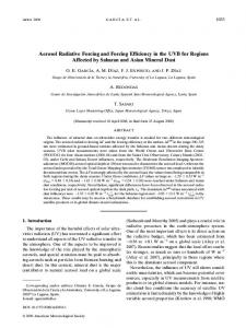
of the retrieved aerosol properties in assessing the TOA DSWARF, considering that the uncertainty in quantifying the aerosol radiative forcing is still quite large, especially for strong aerosol events. A more accurate aerosol characterization in terms of its optical properties is therefore crucial to improving the estimates of the induced climate forcing. The inversion of GOME high spectral resolution measurements is instrumental for the retrieval of aerosol spectral optical quantities, such as spectral extinction, spectral single scattering albedo, and phase function. These quantities are then used to derive the AOT from GEO visible (VIS) broadband measurements, avoiding the use of aerosol models from the literature. The aerosol spectral optical quantities characterizing an aerosol transport event, as well as the AOT obtained at the GEO spatiotemporal scale, are finally used to estimate the DSWARF at the TOA. The physical assumptions made in the radiative transfer calculations are tested with a sensitivity analysis. For this purpose, simulation results of the spectral reflectance, AOT, and TOA DSWARF are analyzed using different literature aerosol models, surface characterization, and vertical profiles of water vapor and ozone. The aim is to account for the impact that these assumptions may have on the retrievals. The method is described in the following section, and section 3 presents the analysis of the sensitivity to the aerosol model, surface type, and molecular vertical profile. Conclusions are proposed in section 4. The applications of the method to significant aerosol transport events are contributed in Costa et al. (2004, hereinafter Part II), which discusses the retrieval of aerosol optical quantities, AOT and TOA DSWARF, and their validation with independent ground-based measurements and satellite retrievals. 2. Method The method is based on LEO and GEO satellite measurements and radiative transfer calculations with the aim of merging the fairly good spectral resolution from GOME and the unrivaled spatial and temporal resolution from GEO satellites, specifically Meteosat. The block diagram of the method is shown in Fig. 1 and full details are given by Costa (2004). All radiative transfer calculations are done using the Second Simulation of the Satellite Signal in the Solar Spectrum model (6S; Vermote et al. 1997). Note that Mie theory is applied to spherical aerosol particles. a. Automated GOME spectral measurement selection The retrieval of aerosol quantities from GOME spectral measurements requires a first step consisting of a spectral and geographical pixel selection where aerosol particles are modeled with fewer uncertainties. GOME measures the solar irradiance and the radiance

DECEMBER 2004

COSTA ET AL.

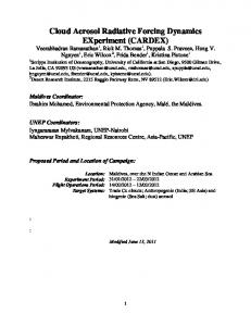
scattered by the earth’s atmosphere and surface in the spectral range between 0.240 and 0.793 mm with a spectral resolution that varies between 0.2 and 0.4 3 10 23 mm and a relative radiometric accuracy of less than 1% (Burrows et al. 1999). Four wavelengths are selected for the present study (at 0.361, 0.421, 0.753, and 0.783 mm) which are characterized by relatively low gas absorption. The geographical areas (pixels) selected to perform the inversions should correspond exclusively to cloudfree areas over the ocean, with overall low reflectance variability that ensures pixel homogeneity. This poses selection problems due to the lack of GOME spectral information in the infrared (IR) spectral region for cloud detection, as well as to the dimension of each GOME pixel (320 3 40 km 2 ). A way of overcoming this limitation involves the use of GEO data so that the GOME geolocation is matched with the GEO best time coincident classified images (maximum time difference is 15 min, often better). The GEO VIS–IR image pairs are classified using the statistical algorithm of Porcu` and Levizzani (1992), originally developed for the Meteosat Visible and InfraRed Imager (MVIRI) channels. The technique is used to discriminate between cloud, land, water (background aerosol contamination), and aerosol (strong aerosol contamination) classes. The different spatial resolution of the GEO and GOME sensors is accounted for when overlapping their respective geolocations by determining which GEO image pixels are located inside each GOME pixel. The latter is marked and selected for the inversion only if the contained GEO satellite image pixels are all classified as water or all classified as aerosol contaminated, thus certifying the pixel spatial homogeneity. Figure 2 shows an example of selection in the case of a strong Saharan dust outbreak from 7 (left panel) to 11 June 1997 (right panel). The pixels bounded with the thicker line survived the selection process: one pixel survives in the first scene (classified as water) and four in the second (all classified as aerosol events). The chance of observing cloud-free ground pixels was estimated for the case studies presented in Part II based on the number of pixels selected for the inversion with respect to the number of analyzed pixels, and it was found that in the worst case around 10% of the analyzed pixels were selected for the inversion. The effect of the GOME pixel dimension, that is, the assumption that the aerosol distribution is horizontally homogeneous over the pixel and the use of a single sun–satellite geometry, was also assessed through the examination of the GEO radiance values that fall inside each selected GOME pixel and the subsequent error propagation on the retrievals. Results of this analysis are presented in section 3. The first European Meteorological Operational polar satellite (METOP), which is scheduled to be ready for launch by mid-2005, carries the GOME-2 instrument that maintains GOME’s spectral characteristics, but greatly increases the spatial resolution to 40 3 40 km 2 .

1801

The present methodology may well be used with GOME-2 data, surely increasing the number of selectable cloud-free homogeneous pixels and improving the confidence in the retrieved mean aerosol model. On the other hand, the use of MODIS or ATSR data in combination with GEO measurements would also increase the number of selectable cloud-free homogeneous pixels, due to the far better spatial resolution of the two sensors with respect to GOME. Their use represents a feasible way of translating the methodology into an operational context and thus contributing to the quantification of aerosol effects on global climate. Note, however, that the confidence in atmospheric correction would be lower because of the broader spectral bands of MODIS and ATSR as compared with GOME high spectral resolution measurements. Therefore, one should use more accurate atmospheric vertical profiles of the gases that have spectral signatures in the bands selected for the aerosol retrievals. b. Aerosol quantities retrieval from GOME Once GOME pixels have been selected, relevant aerosol microphysical parameters can be retrieved by inverting GOME spectral reflectance measurements. In reality, this is a pseudoinversion since it is based on the comparison between the selected measurements and the corresponding simulated spectral reflectance, by varying some of the parameters characterizing the aerosol. Simulations are done considering the ocean surface to be a Lambertian reflector, with a typical spectral reflectance of clear seawater (Viollier 1982) and a tropical type of atmospheric vertical profile (McClatchey et al. 1971). Aerosols are assumed to be characterized by a bimodal lognormal size distribution with a fine and a coarse mode, and a spectral complex refractive index common to both modes. The size distribution and spectral complex refractive index values are taken from the series of climatological aerosol models of Dubovik et al. (2002a), which are based on the analysis of several years of ground-based measurements from the Aerosol Robotic Network (AERONET; Holben et al. 1998) relative to diverse aerosol types and geographic locations. The present GOME spectral reflectance pseudoinversion conducted over wider geographical areas and shorter time periods is then useful in refining these climatological models, which refer to longer time periods and point measurements. The refinement is possible through the variation of some of the size distributions and/or the spectral complex refractive index. The sensitivity of the TOA spectral reflectance, AOT, and TOA DSWARF are investigated with respect to the individual variations of each of the size distribution parameters and the complex refractive index in order to assess which of these parameters most strongly influence the physical quantities under study. Figure 3 presents the TOA spectral reflectance at four wavelengths as a function of the aerosol size distribution parameters (fine- and coarse-mode

1802


modal radii, fine- and coarse-mode standard deviations, and fine-mode percentage density), the complex refractive index (real and imaginary parts, the latter in two spectral regions: 0.35–0.50 and 0.70–0.86 mm), and aerosol optical thickness. This is done for two of the climatological aerosol models described by Dubovik et al. (2002a): Cape Verde (left), representative of desert dust aerosols, and African savannah (right), representative of biomass burning aerosols. The horizontal dashed line in Fig. 3 indicates the spectral reflectance obtained with the climatological model for an AOT value of 0.5. The spectral reflectance variations are obtained by changing the size distribution parameters, the complex refractive index, and the AOT one at a time, and leaving the others fixed by the climatological model, as well as setting the AOT to 0.5. Figure 4 shows the AOT obtained from the GEO radiances, as a function of the aerosol size distribution parameters and complex refractive index for the climatological aerosol models of Fig. 3 (left, Cape Verde; right, African savannah). Also the horizontal dashed line indicates the reference AOT of 0.5, corresponding to the use of the climatological model. As for the previous quantity, the AOT variations are obtained by changing the size distribution parameters and the complex refractive index one at a time, in each case leaving the remaining parameters fixed by the climatological model. Figure 5 illustrates the TOA DSWARF as a function of the aerosol size distribution parameters, complex refractive index, and AOT, for the climatological aerosol models in Fig. 3 (left, Cape Verde; right, African savannah). The horizontal dashed line indicates the TOA DSWARF obtained with the climatological model for an AOT value of 0.5. As before, the TOA DSWARF variations are obtained by changing the size distribution parameters, the complex refractive index, and the AOT one at a time, with the remaining parameters being fixed by the climatological model and with the AOT set to 0.5. The analysis of the graphs in Figs. 3–5 shows that the fine- and coarse-mode standard deviations, as well as the real part of the refractive index, have a small effect on the variation of the spectral reflectance for any of the analyzed wavelengths, on the AOT and on the TOA DSWARF. In most of the cases the sensitivity of the analyzed quantities at the used wavelengths is greater to the fine-mode modal radius than to that of the coarse mode, especially in the cases in which the fraction of smaller particles is greater (biomass burning case). The fine-mode percentage particle density also originates high variations, especially of the spectral re-

VOLUME 43

flectances. The imaginary part of the refractive index in the two spectral regions considered is undoubtedly one of the most important parameters to be investigated, together with the AOT (Figs. 3 and 5), which becomes increasingly important in the case of the spectral reflectance at longer wavelengths. This study allowed for the selection of the parameters that mostly influence the spectral reflectance (measured quantity), as well as the AOT and the TOA DSWARF (the key quantities to be derived). Therefore, these parameters (fine-mode modal radius, fine-mode percentage density of particles, imaginary part of the refractive index in two spectral regions, and AOT) are varied in the aerosol characterization used to simulate the spectral reflectance, which is subsequently compared with the GOME spectral reflectance measurements. The spectral regions considered for the imaginary refractive index are 0.35–0.50 and 0.70–0.86 mm. The variation of the parameters is done via fixed combinations that depend on the aerosol event type, which is imposed a priori depending on the case under study (geographical location is an important indicator, combined with ancillary data such as trajectory analysis). The variation limits are indicated in Tables 1 and 2. The parameters that originate smaller variations of the analyzed quantities (coarse-mode modal radius, fine- and coarse-mode standard deviations, and real part of the refractive index) are fixed by the respective climatological model, which is established each time according to the case study. The percentage density of particles for each mode is related as follows: pd C 5 100 2 pd F ,

(1)

where pd C is the percentage density of particles of the coarse mode and pd F that of the fine particle mode. The distinction between an aerosol event and background aerosol conditions (considered to be described by a maritime aerosol model) is based on the GEO image classification (described in section 2a), which allows for the selection of spatially homogeneous GOME pixels (Fig. 2). If the classification indicates background aerosol contamination within the pixel, the maritime model is chosen; on the contrary, if the classification suggests an aerosol event, the corresponding aerosol model is used according to the case under study. Lookup tables (LUTs) are computed for a number of different geometric conditions and several fixed aerosol models, which are built as explained before, fixing the parameters of the size distribution and complex refractive index and varying the fine-mode modal radius, the →

FIG. 1. Block diagram of the aerosol retrieval method, which is based on the combination of data from LEO and GEO satellites to derive aerosol properties, AOT, and TOA DSWARF. Data from the GOME spectrometer were used. Gray boxes represent the results and black boxes the validation datasets. In the validation process the aerosol optical properties and AOT are checked against retrievals from sun and sky radiance measurements from the ground-based AERONET. The AOT is also compared with the satellite aerosol official POLDER and MODIS products. The upwelling flux at the TOA is compared with space–time-collocated measurements from the Clouds and the Earth’s Radiant Energy System (CERES) TOA flux product.

DECEMBER 2004

COSTA ET AL.

1803

1804


VOLUME 43

FIG. 2. Selection of GOME pixels by overlapping the GOME geolocation and the Meteosat classified pixels. Four classes are distinguished: water (light gray), land (black), cloud (whitish), and aerosol event over water (dark gray). GOME pixels bounded by thick lines delimit the selections. The examples refer to cases over two limited areas for (left) 7 Jun 1997, GOME orbit 110, and (right) 11 Jun 1997, GOME orbit 122.

fine mode percentage density of particles, the imaginary part of the refractive index in two spectral regions (0.35– 0.50 and 0.70–0.86 mm), and the AOT, in the ranges presented in Tables 1 and 2. The measured spectral re-

flectance (the ratio between the upwelling radiance from the earth’s surface and the extraterrestrial solar radiance) corresponding to each selected GOME pixel is compared with the spectral reflectance from the LUTs. First,

FIG. 3. Spectral reflectance at four wavelengths as a function of the aerosol size distribution parameters (fine- and coarse-mode modal radius, fine- and coarse-mode standard deviation, and fine-mode percentage density), complex refractive index, and aerosol optical thickness, for two climatological aerosol models described by Dubovik et al. (2002a): (left) Cape Verde, representative of desert dust aerosols, and (right) African savannah, representative of biomass burning aerosols. The horizontal dashed line indicates the spectral reflectance obtained with the climatological model for an aerosol optical thickness of 0.5. The spectral reflectance variations are obtained by changing the size distribution parameters, complex refractive index, and optical thickness one at a time while the other parameters were fixed by the climatological model and while the AOT was set to 0.5.

DECEMBER 2004

COSTA ET AL.

1805

FIG. 4. Aerosol optical thickness obtained from the GEO radiances as a function of the aerosol size distribution parameters and complex refractive index for the same two climatological aerosol models as in Fig. 3. The horizontal dashed line indicates the reference aerosol optical thickness of 0.5, corresponding to the use of the climatological model. The aerosol optical thickness variations are obtained by changing the size distribution parameters and the complex refractive index one at a time, in each case the remaining parameters being fixed by the climatological model.

the solar and satellite geometries are identified and the corresponding LUT selected, and second a minimization method is applied to measurements and simulations until the best fit is obtained, leading to the retrieval of the aerosol quantities corresponding to that spectrum (pixel), which are given by the fixed combination of the aerosol parameters (Amod el ) that generated the best fit. The chi-square function used for the minimization is

O [r (l ) 2 rs((ll ;) A n

x 2 (Amod el , t a ) 5

G

S

i

i51

mod el

i

i

]

, t a)

2

, (2)

where Amod el are the aerosol models contained in the LUT; t a is the aerosol optical thickness; r G (l i ) and r S (l i ) are the measured and simulated GOME spectral reflectances, respectively; s(l i ) is the standard deviation associated with GOME spectral measurements; and n is the number of selected wavelengths li (four GOME channels). The minimization procedure results in x 2 , 0.1. Figure 6 shows an example of the fitting result for a selected pixel. Note that the use of the climatological aerosol model for Cape Verde (Dubovik et al. 2002a) does not reproduce measurements as adequately as the derived parameters do. The pseudoinversion is performed over all selected GOME pixels. A subsequent spatiotemporal analysis of the inversion results allows for the retrieval of ef-

fective aerosol quantities describing the atmospheric conditions for a certain geographical area and period of time, which replace those from the models in the literature. In all calculations, the aerosol optical quantities (single-scattering albedo, phase function, and extinction coefficient) are automatically obtained assuming spherical aerosol particles; hence, the GOME-derived aerosol microphysics (size distribution and complex refractive index) are used as input for Mie calculations. c. Aerosol optical thickness retrieval from GEO satellite measurements Aerosol optical quantities (single-scattering albedo, phase function, and extinction coefficient) derived from GOME spectral measurements are then combined with data from GEO platforms to retrieve the AOT. Note that the AOT was already retrieved from the minimization process at the GOME pixel scale. By using GEO data the AOT is retrieved at a considerably better spatial resolution, which is suitable for a monitoring strategy over large areas and longer time periods (the MVIRI image repeat cycle is 0.5 h) using the retrieved classes instead of those from climatology. The algorithm can be applied to any GEO satellite

1806


VOLUME 43

FIG. 5. TOA DSWARF as a function of the aerosol size distribution parameters, complex refractive index, and aerosol optical thickness for the same two climatological aerosol models as in Fig. 3. The horizontal dashed line indicates the TOA DSWARF obtained with the climatological model for an aerosol optical thickness of 0.5. The TOA DSWARF variations are obtained by changing the size distribution parameters, complex refractive index, and optical thickness one at a time while the other parameters were fixed by the climatological model and while the AOT was set to 0.5.

for a possible global coverage strategy. The foreseen use of data from the Meteosat Second Generation (MSG) Spinning Enhanced Visible and Infrared Imager (SEVIRI) would contribute to a further improvement with respect to the present MVIRI, since the sensor has a higher temporal, as well as spatial, resolution: 15-min repeat cycle instead of 30 min, and 3 km at nadir instead of 5 km, respectively. The GEO images are classified using the statistical algorithm of Porcu` and Levizzani (1992) to select the cloud-free pixels over the ocean where the AOT will be derived, as well as to distinguish between aerosol event and background aerosol conditions. If the classification indicates background aerosol contamination

on the pixel, then the maritime model is taken. On the contrary, if the classification identifies an aerosol event, the corresponding aerosol model is once more used according to the case under study. For each mean aerosol class obtained from the inversion of the GOME spectral reflectance over a certain geographical area and period, an LUT of the GEO VIS broadband radiance is derived that considers all possible geometric conditions (sun and satellite) and seven AOT values (0.0, 0.1, 0.2, 0.5, 1.0, 1.5, and 2.0). Presently, GEO systems are equipped with a broadband VIS spectral channel (MVIRI, 0.3—1.1 mm; SEVIRI, 0.56–0.71 and 0.74–0.88 mm). The LUT corresponding to each GEO cloud-free pixel is identified taking into account

TABLE 1. Size distribution parameters. The lower and upper limits of the parameters allowed to vary are indicated in boldface. The remaining parameter values are assigned according to the test case under study. Aerosol type

Mode

Modal radius (mm)

Std dev of the modal radius (mm)

Percentage number density of particles

Biomass burning

Fine Coarse Fine Coarse Fine Coarse

R F 5 0.05–0.6 RC R F 5 0.09–0.6 RC R F 5 0.08–0.6 RC

sF sC sF sC sF sC

PdF : 98.0–100.0 Pd C 5 100.0–Pd F Pd F : 96.0–100.0 Pd C 5 100.0–Pd F PdF : 97.0–100.0 Pd C 5 100.0–Pd F

Desert dust Maritime

DECEMBER 2004

1807

COSTA ET AL.

TABLE 2. Complex refractive index parameters. The lower and upper limits of the parameters allowed to vary are indicated in boldface. The real part (nR) is assigned a fixed value according to the test case under study. Spectral complex refractive index

Aerosol type Biomass burning Desert dust Maritime

nR nR nR nR nR nR

2 2 2 2 2 2

(0.005–0.05)i (0.005–0.05)i (0.0008–0.008)i (0.0006–0.006)i (0.0001–0.001)i (0.0001–0.001)i

Spectral regions (mm)

Aerosol optical thickness

0.35–0.50 0.70–0.86 0.35–0.50 0.70–0.86 0.35–0.50 0.70–0.86

0.4–2.0 0.4–2.0 0.0–0.4

the observing geometry and the pixel classification (event or background aerosol type). Subsequently, the AOT corresponding to each of these GEO image pixels is computed by spline interpolation of the GEO radiances stored in the LUT using the GEO radiance measurement value. d. DSWARF assessment from GEO satellite measurements The 6S code computes the downwelling SW flux at the surface, F SURF ; the upwelling spectral reflectance, ↓ TOA rTOA at the TOA. The l↑ ; and the spectral radiance, I l↑ extraterrestrial solar spectral irradiance, F TOA l↓ , values used in the code are taken from Neckel and Labs (1984). The upwelling SW flux at the TOA (F TOA ) is obtained ↑ here from the spatial integration of the TOA spectral radiance [I TOA l↑ (m, f)] computed over a grid of satellite (GEO) zenith (m) and relative azimuth (f) angles and then integrated from 0.25 to 4.0 mm to yield the broadband (SW) flux, applying the following equation:

E [E E 2p

4.0

F ↑TOA 5

0.25

0

11

]

I lTOA ↑ (m, f )m dm df dl.

0

(3)

All fluxes are calculated for a set of possible solar zenith angle (from 08 to 858 with a step of 58) and AOT values (0.0, 0.2, 0.5, 1.0, 1.5, and 2.0), producing LUTs of both the downwelling and upwelling TOA SW fluxes, the net TOA SW flux, and the TOA DSWARF, the last two defined, respectively, as follows: TOA F net 5 F ↓TOA 2 F ↑TOA and

(4)

TOA TOA DF TOA 5 F net( t aerosol ) 2 F net(t 50) ,

(5)

where F TOA is the TOA SW net flux and DF TOA is the net TOA direct SW radiative forcing due to the presence of aerosol particles (TOA DSWARF). After determining the solar zenith angle, the AOT retrieved in the previous section from GEO data is compared with the AOT values contained in the LUTs. In this way, the TOA DSWARF and the TOA SW flux in the spectral region between 0.25 and 4.0 mm are retrieved.

FIG. 6. GOME measurements and simulated spectral reflectance on 11 Jun 1997 using the aerosol model resulting from the fitting process and a desert aerosol model for Cape Verde (Dubovik et al. 2002a): pixel number 1223 was classified as desert type.

3. Sensitivity analysis Some of the physical assumptions made in the radiative transfer calculations are tested with a sensitivity analysis. For this purpose and in order to identify the main uncertainty affecting the radiative quantities entering the present method, the spectral reflectance, the AOT derived from GEO radiances (see computation procedure in section 2c), and the TOA DSWARF are analyzed for a set of possible geometric conditions. The results of these analyses are presented in terms of the differences resulting from adopting different aerosol models from the literature (indicated in Table 3), two different surface optical characterizations [Lambertian versus bidirectional reflectance distribution function (BRDF)], and two different vertical profiles of water vapor and ozone (tropical versus midlatitude winter). In addition, the efficiency of the algorithm proposed to derive the fine-mode modal radius, the fine-mode percentage particle density, the imaginary part of the refractive index in two spectral regions (0.35–0.50 and 0.70–0.86 mm), and the AOT (at the GOME spatial scale) is tested using synthetic GOME measurements, obtained from calculation with the 6S code. The vertical atmospheric profiles adopted for the analysis are the tropical and the midlatitude winter (McClatchey et al. 1971), whose ozone and water vapor profiles are shown in Fig. 7. These profiles may represent extreme conditions for the geographical areas where the algorithm is to be applied (GEO satellite covTABLE 3. Aerosol models from the literature considered in the sensitivity analysis. Aerosol model

Reference

Maritime: Lanai Desert dust: Cape Verde Biomass burning: African savannah

Dubovik et al. (2002a)

1808


FIG. 7. Tropical and midlatitude winter vertical profiles of ozone and water vapor (McClatchey et al. 1971) used in the sensitivity analysis.

erage); therefore, the resulting differences represent the upper limit for real atmospheric conditions. The results obtained with the assumption of a Lambertian ocean surface, considering a typical spectral reflectance characteristic of clear seawater (Viollier 1982), are compared with those retrieved considering a BRDF for the ocean surface, aiming at quantifying the differences between the two cases. The BRDF ocean model contained in 6S (Morel 1988) is used and takes into account wind speed and direction, ocean salinity, and pigment concentration. Mean values of wind speed of 6 m s 21 , wind direction of 458, salinity of 35 ppt, and pigment concentration of 0.3 mg m 23 were adopted. Three climatological aerosol models were considered in the sensitivity analysis since they represent fairly different possible atmospheric aerosol scenarios: maritime, desert, and biomass burning defined by Dubovik et al. (2002a) (see Table 3). Figure 8 shows the graphs of the relative differences of the spectral reflectance obtained when changing the assumptions with respect to the vertical atmospheric profiles, surface type, and aerosol model. Results are shown as a function of wavelength for different solar zenith angles, considering an AOT value of 1.0, a satellite zenith angle of 228, and a relative azimuth angle of 1508. These angles are chosen because they correspond to a typical GOME geometry. The moderately high AOT value (1.0) is used to establish the maximum errors arising from the different assumptions. The gray vertical dashed lines in each graph in Fig. 8 mark the position of the wavelengths considered in the inversion procedure. Results in Fig. 8a refer to simulations of the spectral reflectance considering a Lambertian ocean surface and the desert aerosol model. As for the vertical characterization, two situations are considered: a tropical and a midlatitude winter vertical profile. These results are subtracted and the respective differences converted in percentages with respect to the value obtained

VOLUME 43

with the tropical profile. The analysis shows that the use of such considerably different vertical atmospheric profiles of water vapor and ozone (see Fig. 7) has a moderate impact on the modeled spectral reflectance, depending on the wavelength. The spectral reflectance relative differences are always ,1% (absolute value) for all the wavelengths used (0.361, 0.421, 0.753, and 0.783 mm), as would be reasonably expected since these wavelengths were chosen to avoid gas absorption regions as much as possible. The relative differences of the spectral reflectance presented in Fig. 8b result from considering first the surface as a Lambertian reflector, and second its BRDF. In this case, the atmospheric tropical vertical profile and the desert aerosol model were considered. Relative differences were calculated with respect to values obtained with the Lambertian surface. The results depend on the geometry (solar zenith angle), and in general the resulting differences are lower than 11% (absolute value) in the blue spectral region and 15%–35% (absolute value) in the red spectral region. The spectral reflectance is also analyzed with respect to the considered aerosol model. Figures 8c and 8d illustrate the results obtained when comparing the desert and maritime, and the desert and biomass burning, aerosol models, respectively (see Table 3). In this case, the ocean surface is considered Lambertian and the atmospheric profile is tropical. The spectral reflectance relative differences were calculated with respect to values obtained with the desert aerosol model. The graphs show slightly different behaviors for the two situations. The desert and maritime aerosol models present differences that range between 5% and 30% (absolute value) in the blue spectral region and are generally between 20% and 35% in the red spectral region, except for u 0 5 08, which reaches 60%. When the biomass burning aerosol model is considered, the differences for smaller wavelengths are lower than the previous ones (between 25% and 215%), whereas for the longer wavelengths they are higher, in general between 55% and 70%, and slightly higher for u 0 5 08 as previously discussed, reaching 95%. The analysis of Fig. 8 clearly shows that among the investigated assumptions the aerosol model is the factor that most influences the spectral reflectance. However, the surface characterization may also have an important role, depending on the geometric conditions, as illustrated in Fig. 8b. The AOT absolute differences as a function of the solar zenith angle (obtained from GEO data according to section 2c) are plotted in Fig. 9 for different satellite zenith angles. An AOT reference value of 1.0 is considered, corresponding to the tropical atmospheric profile as an extreme high humidity case, the Lambertian ocean surface, and the desert model in all cases. The AOT differences are obtained by subtracting the values obtained with the different assumptions from the reference AOT value of 1.0. An instrumental random error of 615% of the total GEO signal is considered in the analysis, which stems from the estimation of the Me-

DECEMBER 2004

COSTA ET AL.

1809

FIG. 8. Spectral reflectance relative differences obtained from the different assumptions as a function of wavelength. Simulations are done for an AOT value of 1.0, a satellite zenith angle of 228, and a relative azimuth angle of 1508. Differences refer to (a) tropical–midlatitude winter vertical profiles, (b) Lambertian surface–BRDF consideration, (c) desert–maritime aerosol model, and (d) desert–biomass burning aerosol model. The vertical dashed lines indicate the wavelengths used for the inversion procedure.

teosat errors on calibration [10%; Govaerts (1999)] and spectral response (10% maximum; Y. M. Govaerts 2000, personal communication). Figure 9a shows the AOT differences while considering the midlatitude winter profile instead of the tropical profile used to estimate the reference value. The differences are, in general, within 60.2, except for high solar and satellite zenith angles when the AOT deviates about 20.3 from the AOT reference value of 1.0. The sinusoidal trend is related to the random 615% error considered in the GEO-simulated radiances. The graphs in Fig. 9b show the AOT absolute differences when the surface BRDF

is considered, with respect to the reference values derived when considering the ocean surface as a Lambertian reflector. Results exhibit maximum differences ranging from 20.2 (high solar and satellite zenith angles) up to 0.4, which constitute considerable deviations with respect to the AOT reference value of 1.0. The sinusoidal trend is once more introduced by the random 615% error considered. Figure 9c illustrates the results obtained using the maritime aerosol model as compared with the reference values obtained with the desert aerosol model. A moderate dependence on the geometry is found. The highest AOT differences range from about

1810


VOLUME 43

FIG. 9. AOT differences as a function of the solar zenith angle for different satellite zenith angles. An AOT value of 1.0 is considered corresponding to a reference LUT calculated using the tropical vertical profile, a Lambertian surface type, and the desert aerosol model. Subsequently, another AOT value is calculated using the reference LUT, from the radiance values obtained considering (a) midlatitude vertical profile, (b) surface BRDF, (c) maritime aerosol model, and (d) biomass burning aerosol model. The AOT differences are obtained from the subtraction of this latter value from the reference value of 1.0.

20.3 to 0.6. The plots in Fig. 9d show the AOT absolute differences when the biomass burning aerosol model is assumed, and these differences are compared with the reference value (desert aerosol model). This case is also characterized by high differences in the AOT results with a maximum of 0.8, that is, a deviation of 80% from the reference AOT, and a minimum of 0.1. Analysis of Fig. 9 clearly shows that, among all the investigated possible influences, the aerosol model is the factor that most influences the AOT. Veefkind and de Leeuw (1998) show that an unrealistic aerosol size distribution may introduce substantial errors on the AOT retrievals from 240% to 160%, which is in agreement with the present results. The surface characterization also has a large impact on the AOT that becomes increasingly important for low aerosol loads because the signal received by the satellite is dominated by the surface contribution. The sensitivity analysis of Tanre´ et al. (1997) has demonstrated that an additional surface contribution results in larger AOT values, and that this effect is more important the smaller the AOT values. Figure 10 shows the graphs of the TOA DSWARF

differences as originated with the different assumptions as a function of the AOT for different solar zenith angles. Reference values of the TOA DSWARF are calculated by considering the Lambertian ocean surface, the tropical atmospheric profile, and the desert aerosol model. The vertical dashed gray lines represent the AOT variation limits resulting from the instrumental random error introduced in the GEO-simulated radiances (615%) and from the different assumptions (see Fig. 9). The aim is to quantify the uncertainty in the TOA DSWARF from errors introduced in the AOT calculation from GEO data. Figure 10a illustrates the differences with respect to the reference values when calculations are done considering the midlatitude winter profile. Differences in this case are proportional to the AOT values and are mostly independent of the solar zenith angle, reaching about 15 W m 22 for AOT . 1.8. The AOT uncertainty of 60.2 introduced by the GEO instrumental error and the use of different atmospheric profiles (see Fig. 9a) generates an uncertainty of about 4 W m 22 in the TOA DSWARF difference. The impact of considering the surface BRDF instead of the Lam-

DECEMBER 2004

COSTA ET AL.

1811

FIG. 10. TOA DSWARF absolute differences derived using the various assumptions considered in the text as a function of the aerosol optical thickness for different solar zenith angles. Differences refer to (a) tropical–midlatitude winter vertical profiles, (b) Lambertian surface– BRDF consideration, (c) desert–maritime aerosol model, and (d) maritime–biomass burning aerosol model.

bertian surface is displayed in Fig. 10b, where the highest differences (about 12 W m 22 in absolute values) are observed for AOT . 1.4 and u 0 5 08 or u 0 5 608. For a solar zenith angle u 0 5 458, the differences are generally ,2.5 W m 22 . In Fig. 10b one can see that the propagation of the AOT uncertainty (between 20.2 and 10.4) upon the TOA DSWARF difference is up to about 2 W m 22 , which is lower than the one introduced by the vertical profile. These results are inverted with respect to those presented in Figs. 8 and 9, where the surface was a more important assumption than the gaseous profiles. This is connected to the fact that the TOA DSWARF is obtained from flux calculations [Eqs. (3)– (5)], which are radiative quantities integrated over a broadband SW spectral region (0.25–4.0 mm). In this broadband region important gas absorption bands are included, especially water vapor and ozone and consequently the assumption on the gaseous atmospheric constituents becomes more important. The differences arising from the use of the different aerosol models are reported in Figs. 10c and 10d. The first one refers to the use of a maritime aerosol model against the desert model used in the computation of the reference values.

The differences are proportional to the AOT with maximum values of around 220 W m 22 . The second one corresponds to the comparison between the desert and the biomass burning aerosol models. In this case, the differences are also proportional to the AOT values although with a lower dependence on the solar zenith angle than the one found in the previous case (Fig. 10c). Nevertheless, differences are much higher than in the previous case, with the maximum value is situated around 280 W m 22 , whereas in Fig. 10c the maximum value reached down to 220 W m 22 . In these cases the GEO AOT uncertainties delimited by the vertical dashed lines (20.3 to 10.6 in Fig. 10c and 10.1 to 10.8 in Fig. 10d) generate greater TOA DSWARF difference uncertainties that may reach about 11 W m 22 in the first case (Fig. 10c) and around 30 W m 22 in the second case (Fig. 10d). For all the situations investigated in the present study, the aerosol model is the factor that most influences any of the analyzed radiative quantities: spectral reflectance (Figs. 8c,d), AOT (Figs. 9c,d), and TOA DSWARF (Figs. 10c,d). The retrieval of the effective aerosol quantities is therefore extremely important in order to reduce

1812


the errors in the retrievals of the aerosol load and its direct radiative forcing, particularly for situations of aerosol events. The adoption of one or the other of the atmospheric vertical profiles has a relatively small impact on the retrievals and this implies that the use of latitudinal- and seasonal-dependent atmospheric profiles is a reasonable approximation to be adopted in the present algorithm. The different surface characterizations originate moderate differences in the results that become more significant for low aerosol loads, as reported by Mishchenko et al. (1999). Since the aim of the present algorithm is the study of aerosol events over the ocean generally distinguished by moderately high aerosol contents and low impact of the surface characterization on the TOA DSWARF, the Lambertian ocean surface may be considered a reasonable approximation. Nevertheless, plans call for LUTs to be built that take into consideration the surface BRDF with the aim of improving the accuracy of the methodology. The methodology is tested using synthetic GOME measurements calculated via the 6S code. The synthetic GOME spectral reflectance values are obtained for 231 cases that consider different geometric conditions, aerosol models, and AOT values. The aerosol model parameters and AOT values used to calculate the synthetic GOME measurements are hereinafter referred to as ‘‘true’’ values. First, these synthetic data were given as input to the algorithm without changing any assumptions with respect to those considered in the LUTs and the spectral reflectances were measured error free in order to test the algorithm performance. In this case, the values of the fine-mode modal radius, the fine-mode percentage density, the imaginary part of refractive index in the two spectral regions, and the AOT were perfectly retrieved with 100% of the differences peaking at zero (not shown). Successively, the synthetic data were tested for different assumptions of the surface characterization, and of the atmospheric vertical profiles of water vapor and ozone. In addition, values of the fine-mode modal radius, the fine-mode percentage density of particles, the imaginary part of the refractive index in the two spectral regions (0.35–0.50 and 0.70– 0.86-mm), and the AOT not included in the LUTs were also considered. Last, the assumption that the aerosol is homogeneously distributed horizontally over the GOME pixel and the effect of using a single sun–satellite geometry were also assessed through the investigation of the best time coincident GEO radiance values (maximum time difference of 15 min) enclosed by the geographical coordinates of the corners of each of the GOME pixels selected for inversion. The mean and standard deviation of the GEO radiance distribution inside each of the analyzed GOME pixels were computed. The relative error was obtained from the ratio between the standard deviation and mean values for each of the pixels. More than 800 pixels selected for the case studies presented in Part II were analyzed and the relative errors averaged, obtaining a mean relative error of 8%. It was

VOLUME 43

assumed that this is the error affecting the GOME spectral reflectance; therefore, a random error of 68% was introduced into the synthetic GOME data. The instrumental radiometric calibration error is considered in all cases by introducing a random noise of 61% to the synthetic data, which is reflected in the GOME relative radiometric accuracy of less than 1% (Burrows et al. 1999). The frequency histograms in Fig. 11 show the differences between the ‘‘true’’ values and the results from the present methodology considering the following: 1) a different atmospheric profile from that used to build the LUT (midlatitude winter instead of tropical; black bars) and 2) a different surface characterization (BRDF instead of Lambertian; gray bars). The frequency histograms refer to the fine-mode modal radius, the finemode percentage density, and the imaginary part of the refractive index in the two spectral regions, respectively. For the different vertical profiles, the differences are quite low: about 92% of the fine-mode modal radius differences are within 60.075 mm. As for the fine-mode percentage density, more than 95% of the cases are very well retrieved, the differences between the true and derived values being within 60.005. The differences obtained for the imaginary part of the refractive index are also quite low, that is, about 93% of the values inside the interval 60.0015 for both spectral regions (0.35– 0.50 and 0.70–0.86 mm). When the surface BRDF is considered, the differences are in general higher as would also be expected from the results in the graph in Fig. 8b. The fine-mode modal radius differences present 72% of the cases within 60.075 mm. The fine-mode percentage density is still well retrieved with about 84% of the differences being within 60.005. As for the imaginary part of the refractive index, the differences are within 60.0015 for 78% of the cases in the first spectral region and 81% of the cases in the second spectral region. The performance of the methodology was also tested for situations in which the aerosol models and AOT values were not included in the LUTs calculation, which may often occur. On the other hand, the effect of the large GOME pixel on the assumption that the aerosol is homogeneously distributed horizontally over the GOME pixel and the effect of using a single sun–satellite geometry were also assessed. The frequency histograms in Fig. 12 illustrate the differences between the true values and the results obtained from the present methodology, when 1) the true values are not included in the LUTs (black bars) and 2) a random error of 68% is introduced into the synthetic GOME data to assess the effect of the GOME pixel dimension (gray bars). About 82% of the fine-mode modal radius differences are within 60.075 mm, when the true values are not included in the LUTs, whereas 75% of the values are within 60.075 mm, when the effect of the GOME pixel dimension is considered. The fine-mode percentage density is well retrieved as well with 86% (true values not

DECEMBER 2004

COSTA ET AL.

1813

FIG. 11. Frequency histograms of the differences between the ‘‘true’’ values and the results obtained from the present methodology, considering 1) a different atmospheric profile from that used to build the LUT (midlatitude winter instead of tropical; black bars) and 2) a different surface characterization (BRDF instead of Lambertian; gray bars). The frequency histograms refer to the fine-mode modal radius, fine-mode percentage density, and the imaginary part of the refractive index in the two spectral regions, respectively.

included in the LUTs; black bars) and 95% (effect of the GOME pixel dimension; gray bars) of the differences within 60.015. As to the imaginary part of the refractive index, the frequency histograms are slightly broader when the true values are not included in the LUTs, translating into larger differences between true and retrieved values. Differences are within 60.0015 for 65% of the cases within the first spectral region. About 71% of the cases are within 60.0015 in the second spectral region. The effect of the GOME pixel shows differences within 60.0015 for 86% and 89% of the cases for the first and second spectral regions, respectively.

The graphs in Fig. 13 illustrate the analysis of the AOT derived from GOME measurements together with the aforementioned aerosol quantities. The left panel of Fig. 13 refers to the different atmospheric and surface assumptions, and the right panel is obtained when the true AOT values are not included in the LUTs and when the GOME pixel dimension is considered. Note that once again the AOT is well retrieved when the vertical profile is changed (black bars in Fig. 13, left panel) with more than 90% of the differences situated between 60.075, whereas only about 56% of the differences are within this limit when the surface characterization is changed (gray bars in Fig. 13, left panel). Nevertheless,

1814


VOLUME 43

FIG. 12. Same as in Fig. 11 but for results referring to the case when 1) the true values are not included in the LUTs (black bars) and 2) a random error of 68% is introduced in the synthetic GOME data to assess the effect of the GOME pixel dimension (gray bars).

about 90% of the AOT differences are within 60.175. When the true AOT values are not included in the LUTs (black bars in Fig. 13, right panel), about 81% of the differences are within 60.075, while 78% of the cases are within this limit when the effect of the GOME pixel dimension is accounted for. The above results reflect the differences between the aerosol models used to build the synthetic spectral reflectance and those contained in the LUTs that best fit the synthetic spectra. Note that no interpolation of the LUT values is done, since the aerosol models in the LUTs are fixed. Therefore, the resulting narrow histograms and the peaks near zero are an indication of the

good performance of the algorithm search in the LUT for values closest to the true value. The location of the aerosol layer in the atmosphere, although not considered in the present methodology, is also an important factor affecting the radiative quantities for wavelengths below 0.4 mm (spectral reflectance at 0.361 mm) especially for absorbing aerosols such as desert dust or biomass burning types. Torres et al. (1998) investigated the radiance change relative to the Rayleigh scattering limit at the wavelength of 0.380 mm due to the aerosol layer height for several aerosol models. Their values, relative to the aerosol model that presents the strongest altitude dependence, range from about 215%

DECEMBER 2004

COSTA ET AL.

1815

FIG. 13. Frequency histograms of the differences between the aerosol optical thickness true values and the results obtained from the present methodology, considering (left) a different atmospheric profile from that used to build the LUT (midlatitude winter instead of tropical; black bars) and a different surface characterization (BRDF instead of Lambertian; gray bars) and (right) true values not included in the LUTs (black bars) and a random error of 68%, which is introduced into the synthetic GOME data to assess the effect of the GOME pixel dimension (gray bars).

(at 1.4-km height) to 230% (at 5.8 km) for a surface reflectance of 0.05. However, in order to include the aerosol vertical distribution among the variable parameters, lidar data (backscattering coefficient) and/or measurements from intensive airborne campaigns would be needed, which are not always available. Throughout the present work the aerosol particles are assumed to be spherical. However, the aerosol particle shape may be an issue, especially for desert dust (Dubovik et al 2002a) and also for marine aerosol in lowhumidity atmospheric conditions (Silva et al. 2002). The application of nonspherical theories to satellite-based retrieval algorithms is a difficult task burdening current satellite systems (Wang et al. 2003a). On one hand, satellite observations do not allow for an accurate determination of the particle shape and, on the other hand, even if these shapes were perfectly known, the necessary analytical tools to describe them may not be available. In fact most of the satellite-based algorithms still rely on the use of Mie theory (Tanre´ et al. 1997; Veefkind and de Leeuw 1998; Torres et al. 1998; Torricella et al. 1999; Wang et al. 2003b). Improvements in the retrievals were brought about by the use of groundbased measurements to take into account the effects of aerosol particle shape, but the issue is yet to be resolved (Dubovik et al. 2002b). The integration of nonspherical theories into the methodology in its present state of development would introduce further assumptions on particle shape and consequently further uncertainties

and therefore the Mie theory is used. Nevertheless, planned future developments of the methodology will have to address the particle shape problem, making use of additional satellite and complementary ground-based measurements when necessary. 4. Conclusions A method based on the synergistic use of LEO and GEO satellite measurements is proposed for aerosoltype characterization, AOT retrieval, and TOA DSWARF assessment over the ocean. The scope is to develop a tool for monitoring aerosol events at the GEO time and space scales, while maintaining the accuracy achieved with LEO instruments. The sensitivity analysis performed in order to investigate the possible impact of the instrumental errors as well as of some of the physical assumptions of the method reveals that the investigated radiative quantities are mostly influenced by the assumed aerosol characterization (aerosol model). It is therefore crucial that the aerosol properties introduced in the method reflect as much as possible the real atmospheric aerosol properties. This is perhaps one of the advantages of the present method when compared to others that make use of aerosol models from the literature that are not necessarily adherent to the observed conditions. In addition, the algorithm was tested using synthetic data and its good performance demonstrated, even when the values used to compute

1816


the simulated measurements were not included in the LUTs and when the effects of the GOME pixel dimension were taken into account. Differences arising from considering the ocean BRDF with respect to the reference values (Lambertian ocean surface) are mostly important for background and clean aerosol situations. For higher aerosol loads, a Lambertian ocean is considered to be a reasonable approximation to the real ocean surface. Nevertheless, there is ongoing work aimed at introducing a more accurate surface characterization on the methodology. Note that the sensitivity analysis reports differences corresponding to limit situations and the actual results are often confined in the lowest difference value range. With regard to the different vertical atmospheric profiles of water vapor and ozone that were considered, a relatively small impact on the retrievals is found. The use of latitudinaland seasonal-dependent atmospheric profiles, if collocated data are not available, can be adopted as a reasonable approximation. The aerosol layer height and the nonsphericity of aerosol particles such as desert dust are not presently considered by the methodology, although they may introduce important errors in the retrievals. Further work is planned to include these issues on the retrievals. The reader is directed once more to Part II of this work for a presentation of several case studies. Acknowledgments. Funding was provided by the Portuguese Foundation for Science and Technology under Grant POCTI/CTA/42917/2001. One of the authors (VL) acknowledges support by the Italian Space Agency under the grant Sinergia GERB-SEVIRI nello studio del bilancio radiativo a scala regionale e locale. The senior author was supported by the Subprograma Cieˆncia e Tecnologia do 28 Quadro Comunita´rio de Apoio. Three anonymous reviewers significantly contributed to the improvement of the manuscript and are gratefully recognized. REFERENCES Bartoloni, A., P. Colandrea, R. Loizzo, M. Mochi, F. Pascuali, N. Santantonio, E. Zappitelli, and M. Cervino, 2000: SYSGOME: Processing chain for aerosol optical thickness product generation at I-PAF. Proc. 2000 EUMETSAT Meteorological Satellite Data Users’ Conf., EUM P 29, Bologna, Italy, 460–467. Burrows, J. P., and Coauthors, 1999: The Global Ozone Monitoring Experiment (GOME): Mission concept and first scientific results. J. Atmos. Sci., 56, 151–175. Costa, M. J., 2004: Aerosol and cloud satellite remote sensing: Monitoring and modelling using passive radiometers. Ph.D. thesis, University of E´vora, E´vora, Portugal, 233 pp. ——, M. Cervino, E. Cattani, F. Torricella, V. Levizzani, A. M. Silva, and S. Melani, 2002: Aerosol characterization and optical thickness retrievals using GOME and METEOSAT satellite data. Meteor. Atmos. Phys., 81, 289–298. ——, V. Levizzani, and A. M. Silva, 2004: Aerosol characterization and direct radiative forcing assessment over the ocean. Part II: Application to test cases and validation. J. Appl. Meteor., 43, 1818–1833.

VOLUME 43

Dubovik, O., B. N. Holben, T. F. Eck, A. Smirnov, Y. J. Kaufman, M. D. King, D. Tanre´, and I. Slutsker, 2002a: Variability of absorption and optical properties of key aerosol types observed in worldwide locations. J. Atmos. Sci., 59, 590–608. ——, ——, T. Lapyonok, A. Sinyuk, M. I. Mishchenko, P. Yang, and I. Slutsker, 2002b: Non-spherical aerosol retrieval method employing light scattering by spheroids. Geophys. Res. Lett., 29, 1415, doi:10.1029/2001GL014506. Goloub, P., D. Tanre´, J. L. Deuze´, M. Herman, A. Marchand, and F.M. Bre´on, 1999: Validation of the first algorithm for deriving the aerosol properties over the ocean using the POLDER/ADEOS measurements. IEEE Trans. Geosci. Remote Sens., 37, 1586– 1596. Govaerts, Y. M., 1999: Correction of the Meteosat-5 and -6 radiometer solar channel spectral response with the Meteosat-7 sensor spectral characteristics. Int. J. Remote Sens., 20, 3677–3682. Griggs, M., 1979: Satellite observations of atmospheric aerosols during the EOMET cruise. J. Atmos. Sci., 36, 695–698. Holben, B. N., and Coauthors, 1998: AERONET—A federated instrument network and data archive for aerosol characterization. Remote Sens. Environ., 66, 1–16. Houghton, J. T., Y. Ding, D. J. Griggs, M. Noguer, P. J. van der Linden, and D. Xiaosu, Eds., 2001. Climate Change 2001: The Scientific Basis. Cambridge University Press, 881 pp. Karyampudi, V. M., and Coauthors, 1999: Validation of the Saharan dust plume conceptual model using lidar, Meteosat, and ECMWF data. Bull. Amer. Meteor. Soc., 80, 1045–1075. King, M., Y. J. Kaufman, D. Tanre´, and T. Nakajima, 1999: Remote sensing of tropospheric aerosols from space: Past, present, and future. Bull. Amer. Meteor. Soc., 80, 2229–2259. Leroy, M., and Coauthors, 1997: Retrieval of atmospheric properties and surface bidirectional reflectances over land from POLDER/ ADEOS. J. Geophys. Res., 102, 17 023–17 037. McClatchey, R. A., W. Fenn, J. E. A. Selby, F. E. Volz, and J. S. Garing, 1971: Optical properties of the atmosphere. Environmental Research Paper 354, Air Force Cambridge Research Laboratories AFCRL-TR-71-0279, Hanscom Air Force Base, Bedford, MA, 85 pp. Mishchenko, M., I. Geogdzhayev, B. Cairns, W. Rossow, and A. Lacis, 1999: Aerosol retrievals over the ocean by use of channels 1 and 2 AVHRR data: Sensitivity analysis and preliminary results. Appl. Opt., 38, 7325–7341. Morel, A., 1988: Optical modelling of the upper ocean in relation to its biogenous matter content (Case I Waters). J. Geophys. Res., 93, 10 479–10 768. Moulin, C., F. Guillard, F. Dulac, and C. E. Lambert, 1997: Longterm daily monitoring of Saharan dust load over ocean using METEOSAT ISCCP-B2 data: 1. Methodology and preliminary results for 1983–1994 in the Mediterranean. J. Geophys. Res., 102, 16 947–16 958. Neckel, H., and D. Labs, 1984: The solar radiation between 3300 and 12500. Solar Phys., 90, 205–258. Porcu`, F., and V. Levizzani, 1992: Cloud classification using METEOSAT VIS-IR imagery. Int. J. Remote Sens., 13, 893–909. Ramon, D., R. Ramananaherisoa, R. Santer, M. Chami, J. Fischer, E. Dilligeard, and T. Heinneman, 1999: Characterisation of aerosols over land from space sensors. Final Rep. for the CEO, European Commission Contribution 14055-1998-06F1ED ISP FR, 139 pp. Rosenfeld, D., 1999: TRMM observed first direct evidence of smoke from forest fires inhibiting rainfall. Geophys. Res. Lett., 26, 3105–3108. ——, 2000: Suppression of rain and snow by urban and industrial air pollution. Science, 287, 1793–1796. Silva, A. M., L. Bugalho, M. J. Costa, W. Hoyningen-Huene, T. Schmidt, J. Heitzenberg, and S. Henning, 2002: Aerosol optical properties from columnar data during the second Aerosol Characterization Experiment on the south coast of Portugal. J. Geophys. Res., 107, 4642, doi:10.1029/2002JD002196. Tanre´, D., Y. J. Kaufman, M. Herman, and S. Mattoo, 1997: Remote

DECEMBER 2004

COSTA ET AL.

sensing of aerosol properties over oceans using the MODIS/EOS spectral radiances. J. Geophys. Res., 102, 16 971–16 988. Torres, O., P. K. Bhartia, J. R. Herman, Z. Ahmad, and J. Gleason, 1998: Derivation of aerosol properties from satellite measurements of backscattered ultraviolet radiation: Theoretical basis. J. Geophys. Res., 103, 17 099–17 110. Torricella, F., E. Cattani, M. Cervino, R. Guzzi, and C. Levoni, 1999: Retrieval of aerosol properties over the ocean using GOME measurements: Method and applications to test cases. J. Geophys. Res., 104, 12 085–12 098. Veefkind, J., and G. de Leeuw, 1998: A new algorithm to determine the spectral aerosol optical depth from satellite radiometer measurements. J. Aerosol Sci., 29, 1237–1248.

1817

Vermote, E. F., D. Tanre´, J.-L. Deuze, M. Herman, and J.-J. Morcrette, 1997: Second Simulation of the Satellite Signal in the Solar Spectrum: An overview. IEEE Trans. Geosci. Remote Sens., 35, 675–686. Viollier, M., 1982: Radiometric calibration of the Coastal Zone Color Scanner on Nimbus 7: A proposed adjustment. Appl. Opt., 21, 1142–1145. Wang, J., X. Liu, S. Christopher, J. Reid, E. Reid, and H. Maring, 2003a: The effects of nonsphericity on geostationary satellite retrievals of dust aerosols. Geophys. Res. Lett., 30, 2293, doi: 10.1029/2003GL018697. ——, and Coauthors, 2003b: GOES-8 retrieval of dust aerosol optical thickness over the Atlantic Ocean during PRIDE. J. Geophys. Res., 108, 8595, doi:10.1029/2002JD002494.