Department of Computer Science, University at Albany - State University of New York, Albany,. NY 12222. Email: {davidson,ravi}@cs.albany.edu. Abstract.
Agglomerative Hierarchical Clustering with Constraints: Theoretical and Empirical Results Ian Davidson1 and S. S. Ravi1 Department of Computer Science, University at Albany - State University of New York, Albany, NY 12222. Email: {davidson,ravi}@cs.albany.edu.
Abstract. We explore the use of instance and cluster-level constraints with agglomerative hierarchical clustering. Though previous work has illustrated the benefits of using constraints for non-hierarchical clustering, their application to hierarchical clustering is not straight-forward for two primary reasons. First, some constraint combinations make the feasibility problem (Does there exist a single feasible solution?) NP-complete. Second, some constraint combinations when used with traditional agglomerative algorithms can cause the dendrogram to stop prematurely in a dead-end solution even though there exist other feasible solutions with a significantly smaller number of clusters. When constraints lead to efficiently solvable feasibility problems and standard agglomerative algorithms do not give rise to dead-end solutions, we empirically illustrate the benefits of using constraints to improve cluster purity and average distortion. Furthermore, we introduce the new γ constraint and use it in conjunction with the triangle inequality to considerably improve the efficiency of agglomerative clustering.
1 Introduction and Motivation Hierarchical clustering algorithms are run once and create a dendrogram which is a tree structure containing a k-block set partition for each value of k between 1 and n, where n is the number of data points to cluster allowing the user to choose a particular clustering granularity. Though less popular than non-hierarchical clustering there are many domains [16] where clusters naturally form a hierarchy; that is, clusters are part of other clusters. Furthermore, the popular agglomerative algorithms are easy to implement as they just begin with each point in its own cluster and progressively join the closest clusters to reduce the number of clusters by 1 until k = 1. The basic agglomerative hierarchical clustering algorithm we will improve upon in this paper is shown in Figure 1. However, these added benefits come at the cost of time and space efficiency since a typical implementation with symmetrical distances requires Θ(mn2 ) computations, where m is the number of attributes used to represent each instance. In this paper we shall explore the use of instance and cluster level constraints with hierarchical clustering algorithms. We believe the use of such constraints with hierarchical clustering is the first though there exists work that uses spatial constraints to find specific types of clusters and avoid others [14, 15]. The similarly named constrained hierarchical clustering [16] is actually a method of combining partitional and hierarchical clustering algorithms; the method does not incorporate apriori constraints. Recent work
Agglomerative(S = {x1 , . . . , xn }) returns Dendrogramk for k = 1 to |S|. 1. Ci = {xi }, ∀i. 2. for k = |S| down to 1 Dendrogramk = {C1 , . . . , Ck } d(i, j) = D(Ci , Cj ), ∀i, j; l, m = argmina,b d(a, b). Cl = Join(Cl , Cm ); Remove(Cm ). endloop Fig. 1. Standard Agglomerative Clustering
[1, 2, 12] in the non-hierarchical clustering literature has explored the use of instancelevel constraints. The must-link and cannot-link constraints require that two instances must both be part of or not part of the same cluster respectively. They are particularly useful in situations where a large amount of unlabeled data to cluster is available along with some labeled data from which the constraints can be obtained [12]. These constraints were shown to improve cluster purity when measured against an extrinsic class label not given to the clustering algorithm [12]. The δ constraint requires the distance between any pair of points in two different clusters to be at least δ. For any cluster Ci with two or more points, the ǫ-constraint requires that for each point x ∈ Ci , there must be another point y ∈ Ci such that the distance between x and y is at most ǫ. Our recent work [4] explored the computational complexity (difficulty) of the feasibility problem: Given a value of k, does there exist at least one clustering solution that satisfies all the constraints and has k clusters? Though it is easy to see that there is no feasible solution for the three cannot-link constraints CL(a,b),CL(b,c),CL(a,c) for k < 3, the general feasibility problem for cannot-link constraints is NP-complete by a reduction from the graph coloring problem. The complexity results of that work, shown in Table 1 (2nd column), are important for data mining because when problems are shown to be intractable in the worst-case, we should avoid them or should not expect to find an exact solution efficiently. We begin this paper by exploring the feasibility of agglomerative hierarchical clustering under the above four mentioned instance and cluster-level constraints. This problem is significantly different from the feasibility problems considered in our previous work since the value of k for hierarchical clustering is not given. We then empirically show that constraints with a modified agglomerative hierarchical algorithm can improve the quality and performance of the resultant dendrogram. To further improve performance we introduce the γ constraint which when used with the triangle inequality can yield large computation saving that we have bounded in the best and average case. Finally, we cover the interesting result of an irreducible clustering. If we are given a feasible clustering with kmax clusters then for certain combination of constraints joining the two closest clusters may yield a feasible but “dead-end” solution with k clusters from which no other feasible solution with less than k clusters can be obtained, even though they are known to exist. Therefore, the created dendrograms may be incomplete. Throughout this paper D(x, y) denotes the Euclidean distance between two points and D(X, Y ) the Euclidean distance between the centroids of two groups of instances.
We note that the feasibility and irreducibility results (Sections 2 and 5) are not necessarily for Euclidean distances and are hence applicable for single and complete linkage clustering while the γ-constraint to improve performance (Section 4) is applicable to any metric space.
Constraint Given k Unspecified k Unspecified k - Deadends? Must-Link P [9, 4] P No Cannot-Link NP-complete [9, 4] P Yes δ-constraint P [4] P No ǫ-constraint P [4] P No Must-Link and δ P [4] P No Must-Link and ǫ NP-complete [4] P No δ and ǫ P [4] P No Must-Link, Cannot-Link, NP-complete [4] NP-complete Yes δ and ǫ Table 1. Results for Feasibility Problems for a Given k (partitional clustering) and Unspecified k (hierarchical clustering)
2 Feasibility for Hierarchical Clustering In this section, we examine the feasibility problem for several different types of constraints, that is, the problem of determining whether the given set of points can be partitioned into clusters so that all the specified constraints are satisfied. Definition 1. Feasibility problem for Hierarchical Clustering (F HC) Instance: A set S of nodes, the (symmetric) distance d(x, y) ≥ 0 for each pair of nodes x and y in S and a collection C of constraints. Question: Can S be partitioned into subsets (clusters) so that all the constraints in C are satisfied? When the answer to the feasibility question is “yes”, the corresponding algorithm also produces a partition of S satisfying the constraints. We note that the F HC problem considered here is significantly different from the constrained non-hierarchical clustering problem considered in [4] and the proofs are different as well even though the end results are similar. For example in our earlier work we showed intractability results for some constraint types using a straightforward reduction from the graph coloring problem. The intractability proof used in this work involves more elaborate reductions. For the feasibility problems considered in [4], the number of clusters is in effect, another constraint. In the formulation of F HC, there are no constraints on the number of clusters, other than the trivial ones (i.e., the number of clusters must be at least 1 and at most |S|). We shall in this section begin with the same constraints as those considered in [4]. They are: (a) Must-Link (ML) constraints, (b) Cannot-Link (CL) constraints, (c) δ constraint and (d) ǫ constraint. In later sections we shall introduce another cluster-level
constraint to improve the efficiency of the hierarchical clustering algorithms. As observed in [4], a δ constraint can be efficiently transformed into an equivalent collection of ML-constraints. Therefore, we restrict our attention to ML, CL and ǫ constraints. We show that for any pair of these constraint types, the corresponding feasibility problem can be solved efficiently. The simple algorithms for these feasibility problems can be used to seed an agglomerative or divisive hierarchical clustering algorithm as is the case in our experimental results. However, when all three types of constraints are specified, we show that the feasibility problem is NP-complete and hence finding a clustering, let alone a good clustering, is computationally intractable. 2.1 Efficient Algorithms for Certain Constraint Combinations When the constraint set C contains only ML and CL constraints, the F HC problem can be solved in polynomial time using the following simple algorithm. 1. Form the clusters implied by the ML constraints. (This can be done by computing the transitive closure of the ML constraints as explained in [4].) Let C1 , C2 , . . ., Cp denote the resulting clusters. 2. If there is a cluster Ci (1 ≤ i ≤ p) with nodes x and y such that x and y are also involved in a CL constraint, then there is no solution to the feasibility problem; otherwise, there is a solution. When the above algorithm indicates that there is a feasible solution to the given F HC instance, one such solution can be obtained as follows. Use the clusters produced in Step 1 along with a singleton cluster for each node that is not involved in an ML constraint. Clearly, this algorithm runs in polynomial time. We now consider the combination of CL and ǫ constraints. Note that there is always a trivial solution consisting of |S| singleton clusters to the F HC problem when the constraint set involves only CL and ǫ constraints. Obviously, this trivial solution satisfies both CL and ǫ constraints, as the latter constraint only applies to clusters containing two or more instances. The F HC problem under the combination of ML and ǫ constraints can be solved efficiently as follows. For any node x, an ǫ-neighbor of x is another node y such that D(x, y) ≤ ǫ. Using this definition, an algorithm for solving the feasibility problem is: 1. Construct the set S ′ = {x ∈ S : x does not have an ǫ-neighbor}. 2. If some node in S ′ is involved in an ML constraint, then there is no solution to the F HC problem; otherwise, there is a solution. When the above algorithm indicates that there is a feasible solution, one such solution is to create a singleton cluster for each node in S ′ and form one additional cluster containing all the nodes in S − S ′ . It is easy to see that the resulting partition of S satisfies the ML and ǫ constraints and that the feasibility testing algorithm runs in polynomial time. The following theorem summarizes the above discussion and indicates that we can extend the basic agglomerative algorithm with these combinations of constraint types to perform efficient hierarchical clustering. However, it does not mean that we can always use traditional agglomerative clustering algorithms as the closest-clusterjoin operation can yield dead-end clustering solutions as discussed in Section 5.
Theorem 1. The F HC problem can be solved efficiently for each of the following combinations of constraint types: (a) ML and CL (b) CL and ǫ and (c) ML and ǫ. ⊓ ⊔ 2.2 Feasibility Under ML, CL and ǫ Constraints In this section, we show that the F HC problem is NP-complete when all the three constraint types are involved. This indicates that creating a dendrogram under these constraints is an intractable problem and the best we can hope for is an approximation algorithm that may not satisfy all constraints. The NP-completeness proof uses a reduction from the One-in-Three 3SAT with positive literals problem (O PL) which is known to be NP-complete [11]. For each instance of the O PL problem we can construct a constrained clustering problem involving ML, CL and ǫ constraints. Since complexity results are worse case, the existence of just these problems is sufficient for theorem 2. One-in-Three 3SAT with Positive Literals (O PL) Instance: A set C = {x1 , x2 , . . . , xn } of n Boolean variables, a collection Y = {Y1 , Y2 , . . . , Ym } of m clauses, where each clause Yj = (xj1 , xj2 , xj3 } has exactly three non-negated literals. Question: Is there an assignment of truth values to the variables in C so that exactly one literal in each clause becomes true? Theorem 2. The F HC problem is NP-complete when the constraint set contains ML, CL and ǫ constraints. The proof of the above theorem is somewhat lengthy and is omitted because of space reasons. (The proof appears in an expanded technical report version of this paper [5] that is available on-line.)
3 Using Constraints for Hierarchical Clustering: Algorithm and Empirical Results
Data Set
Distortion Purity Unconstrained Constrained Unconstrained Constrained Iris 3.2 2.7 58% 66% Breast 8.0 7.3 53% 59% Digit (3 vs 8) 17.1 15.2 35% 45% Pima 9.8 8.1 61% 68% Census 26.3 22.3 56% 61% Sick 17.0 15.6 50% 59% Table 2. Average Distortion per Instance and Average Percentage Cluster Purity over Entire Dendrogram
To use constraints with hierarchical clustering we change the algorithm in Figure 1 to factor in the above discussion. As an example, a constrained hierarchical clustering algorithm with must-link and cannot-link constraints is shown in Figure 2. In
this section we illustrate that constraints can improve the quality of the dendrogram. We purposefully chose a small number of constraints and believe that even more constraints will improve upon these results. We will begin by investigating must-link and cannot-link constraints using six real world UCI datasets. For each data set we clustered all instances but removed the labels from 90% of the data (Su ) and used the remaining 10% (Sl ) to generate constraints. We randomly selected two instances at a time from Sl and generated must-link constraints between instances with the same class label and cannot-link constraints between instances of differing class labels. We repeated this process twenty times, each time generating 250 constraints of each type. The performance measures reported are averaged over these twenty trials. All instances with missing values were removed as hierarchical clustering algorithms do not easily handle such instances. Furthermore, all non-continuous columns were removed as there is no standard distance measure for discrete columns.
ConstrainedAgglomerative(S,ML,CL) returns Dendrogrami , i = kmin ... kmax Notes: In Step 5 below, the term “mergeable clusters” is used to denote a pair of clusters whose merger does not violate any of the given CL constraints. The value of t at the end of the loop in Step 5 gives the value of kmin . 1. Construct the transitive closure of the ML constraints (see [4] for an algorithm) resulting in r connected components M1 , M2 , . . ., Mr . 2. If two points {x,Sy} are both a CL and ML constraint then output “No Solution” and stop. r 3. Let S1 = S − ( i=1 Mi ). Let kmax = r + |S1 |. 4. Construct an initial feasible clustering with kmax clusters consisting of the r clusters M1 , . . ., Mr and a singleton cluster for each point in S1 . Set t = kmax . 5. while (there exists a pair of mergeable clusters) do (a) Select a pair of clusters Cl and Cm according to the specified distance criterion. (b) Merge Cl into Cm and remove Cl . (The result is Dendrogramt−1 .) (c) t = t − 1. endwhile Fig. 2. Agglomerative Clustering with ML and CL Constraints
Table 2 illustrates the quality improvement that the must-link and cannot-link constraints provide. Note that we compare the dendrograms for k values between kmin and kmax . For each corresponding level in theP unconstrained and constrained dendrogram n we measure the average distortion (1/n ∗ i=1 D(xi − Cf (xi ) ), where f (xi ) returns the index of the closest cluster to xi ) and present the average over all levels. It is important to note that we are not claiming that agglomerative clustering has distortion as an objective function, rather that it is a good measure of cluster quality. We see that the distortion improvement is typically of the order of 15%. We also see that the average percentage purity of the clustering solution as measured by the class label purity improves. The cluster purity is measured against the extrinsic class labels. We believe these improvement are due to the following. When many pairs of clusters have simi-
lar short distances, the must-link constraints guide the algorithm to a better join. This type of improvement occurs at the bottom of the dendrogram. Conversely, towards the top of the dendrogram the cannot-link constraints rule out ill-advised joins. However, this preliminary explanation requires further investigation which we intend to address in the future. In particular, a study of the most informative constraints for hierarchical clustering remains an open question, though promising preliminary work for the area of non-hierarchical clustering exists [2]. We next use the cluster-level δ constraint with an arbitrary value to illustrate the great computational savings that such constraints offer. Our earlier work [4] explored ǫ and δ constraints to provide background knowledge towards the “type” of clusters we wish to find. In that paper we explored their use with the Aibo robot to find objects in images that were more than 1 foot apart as the Aibo can only navigate between such objects. For these UCI data sets no such background knowledge exists and how to set these constraint values for non-spatial data remains an active research area. Hence we test these constraints with arbitrary values. We set δ equal to 10 times the average distance between a pair of points. Such a constraint will generate hundreds even thousands of must-link constraints that can greatly influence the clustering results and algorithm efficiency as shown in Table 3. We see that the minimum improvement was 50% (for Census) and nearly 80% for Pima. This improvement is due to the constraints effectively creating a pruned dendrogram by making kmax ≪ n.
Data Set Unconstrained Constrained Iris 22,201 3,275 Breast 487,204 59,726 Digit (3 vs 8) 3,996,001 990,118 Pima 588,289 61,381 Census 2,347,305,601 563,034,601 Sick 793,881 159,801 Table 3. The Rounded Mean Number of Pair-wise Distance Calculations for an Unconstrained and Constrained Clustering using the δ constraint
4 Using the γ Constraint to Improve Performance In this section we introduce a new constraint, the γ constraint and illustrate how the triangle inequality can be used to further improve the run-time performance of agglomerative hierarchical clustering. Though this improvement does not affect the worst-case analysis, we can perform a best case analysis and an expected performance improvement using the Markov inequality. Future work will investigate if tighter bounds can be found. There exists other work involving the triangle inequality but not constraints for non-hierarchical clustering [6] as well as for hierarchical clustering [10]. Definition 2. (The γ Constraint For Hierarchical Clustering) Two clusters whose geometric centroids are separated by a distance greater than γ cannot be joined.
IntelligentDistance (γ, C = {C1 , . . . , Ck }) returns d(i, j) ∀i, j. 1. for i = 2 to n − 1 d1,i = D(C1 , Ci ) endloop 2. for i = 2 to n − 1 for j = i + 1 to n − 1 dˆi,j = |d1,i − d1,j | if dˆi,j > γ then di,j = γ + 1 ; do not join else di,j = D(xi , xj ) endloop endloop 3. return di,j , ∀i, j. Fig. 3. Function for Calculating Distances Using the γ Constraint and the Triangle Inequality.
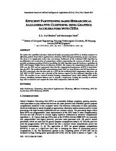
The γ constraint allows us to specify how geometrically well separated the clusters should be. Recall that the triangle inequality for three points a, b, c refers to the expression |D(a, b) − D(b, c)| ≤ D(a, c) ≤ D(a, b) + D(c, b) where D is the Euclidean distance function or any other metric function. We can improve the efficiency of the hierarchical clustering algorithm by making use of the lower bound in the triangle inequality and the γ constraint. Let a, b, c now be cluster centroids and we wish to determine the closest two centroids to join. If we have already computed D(a, b) and D(b, c) and the value |D(a, b) − D(b, c)| exceeds γ, then we need not compute the distance between a and c as the lower bound on D(a, c) already exceeds γ and hence a and c cannot be joined. Formally the function to calculate distances using geometric reasoning at a particular dendrogram level is shown in Figure 3. Central to the approach is that the distance between a central point (c) (in this case the first) and every other point is calculated. Therefore, when bounding the distance between two instances (a, b) we effectively calculate a triangle with two edges with know lengths incident on c and thereby lower bound the distance between a and b. How to select the best central point and the use of multiple central points remains future important research. If the triangle inequality bound exceeds γ, then we save making m floating point power calculations if the data points are in m dimensional space. As mentioned earlier we have no reason to believe that there will be at least one situation where the triangle inequality saves computation in all problem instances; hence in the worst case, there is no performance improvement. But in practice it is expected to occur and hence we can explore the best and expected case results. 4.1 Best Case Analysis for Using the γ constraint Consider the n points to cluster {x1 , ..., xn }. The first iteration of the agglomerative hierarchical clustering algorithm using symmetrical distances is to compute the distance between each point and every other point. This involves the computation (D(x1 , x2 ), D(x1 , x3 ),..., D(x1 , xn )),..., (D(xi , xi+1 ), D(xi , xi+2 ),...,D(xi , xn )),..., (D(xn−1 , xn )), which corresponds to an arithmetic series n − 1 + n − 2 + . . . + 1 of computations. Thus for agglomerative hierarchical clustering using symmetrical distances the number of distance computations is n(n − 1)/2 for the base level. At the next level we need only recalculate the distance between the newly created cluster and the remain-
x1
x2
x3
x4
x5
x3
x4
x4
x5
x5
x5
Fig. 4. A Simple Illustration for a Five Instance Problem of How the Triangular Inequality Can Save Distance Computations
ing n − 2 points and so on. Therefore, the total number of distance calcluation is n(n − 1)/2 + (n − 1)(n − 2)/2 = (n − 1)2 . We can view the base level calculation pictorially as a tree construction as shown in Figure 4. If we perform the distance calculation at the first level of the tree then we can obtain bounds using the triangle inequality for all branches in the second level. This is as bounding the distance between two points requires the distance between these points and a common point, which in our case is x1 . Thus in the best case there are only n − 1 distance computations instead of (n − 1)2 . 4.2 Average Case Analysis for Using the γ constraint However, it is highly unlikely that the best case situation will ever occur. We now focus on the average case analysis using the Markov inequality to determine the expected performance improvement which we later empirically verify. Let ρ be the average distance between any two instances in the data set to cluster. The triangle inequality provides a lower bound; if this bound exceeds γ, computational savings will result. We can bound how often this occurs if we can express γ in terms of ρ, hence let γ = cρ. Recall that the general form of the Markov inequality is: P (X = x ≥ a) ≤ E(X) a , where x is a single value of the continuous random variable X, a is a constant and E(X) is the expected value of X. In our situation since X is distance between two points chosen at random, E(X) = ρ and γ = a = cρ as we wish to determine when the distance will exceed γ. Therefore, at the lowest level of the tree (k = n) then the number ρ = n cρ = n/c, of times the triangle inequality will save us computation time is n E(X) a indicating a saving of a factor of 1/c at this lowest level. As the Markov inequality is a rather weak bound then in practice the saving may be substantially different as we shall see in our empirical section. The computation saving that are obtained at the bottom of the dendrogram are reflected at higher levels of the dendrogram. When growing the entire dendrogram we will save at least n/c + (n − 1)/c . . . +1/c distance calculations. This is an arithmetic sequence with the additive constant being 1/c and hence the total expected computations saved is at least n/2(2/c + (n − 1)/c) = (n2 + n)/2c. As the total computations for regular hierarchical clustering is (n − 1)2 , the computational saving is expected to be by a approximately a factor of 1/2c. Consider the 150 instance IRIS data set (n=150) where the average distance (with attribute value ranges all being normalized to between 0 and 1) between two instances is 0.6; that is, ρ = 0.6. If we state that we do not wish to join clusters whose centroids are separated by a distance greater than 3.0, then γ = 3.0 = 5ρ. By not using
the γ constraint and the triangle inequality the total number of computations is 22201, and the number of computations that are saved is at least (1502 + 150)/10 = 2265; hence the saving is about 10%. We now show that the γ constraint can be used to improve efficiency of the basic agglomerative clustering algorithm. Table 4 illustrates the improvement that using a γ constraint equal to five times the average pairwise instance distance. We see that the average improvement is consistent with the average case bound derived above.
Data Set Unconstrained Using γ Constraint Iris 22,201 19,830 Breast 487,204 431,321 Digit (3 vs 8) 3,996,001 3,432,021 Pima 588,289 501,323 Census 2,347,305,601 1,992,232,981 Sick 793,881 703,764 Table 4. The Efficiency of Using the Geometric Reasoning Approach from Section 4 (Rounded Mean Number of Pair-wise Distance Calculations.)
5 Constraints and Irreducible Clusterings In the presence of constraints, the set partitions at each level of the dendrogram must be feasible. We have formally shown that if kmax is the maximum value of k for which a feasible clustering exists, then there is a way of joining clusters to reach another clustering with kmin clusters [5]. In this section we ask the following question: will traditional agglomerative clustering find a feasible clustering for each value of k between kmax and kmin ? We formally show that in the worse case, for certain types of constraints (and combinations of constraints), if mergers are performed in an arbitrary fashion (including the traditional hierarchical clustering algorithm, see Figure 1), then the dendrogram may prematurely dead-end. A premature dead-end implies that the dendrogram reaches a stage where no pair of clusters can be merged without violating one or more constraints, even though other sequences of mergers may reach significantly higher levels of the dendrogram. We use the following definition to capture the informal notion of a “premature end” in the construction of a dendrogram. How to perform agglomerative clustering in these dead-end situations remains an important open question. Definition 3. A feasible clustering C = {C1 , C2 , . . ., Ck } of a set S is irreducible if no pair of clusters in C can be merged to obtain a feasible clustering with k − 1 clusters. The remainder of this section examines the question of which combinations of constraints can lead to premature stoppage of the dendrogram. We first consider each of the ML, CL and ǫ-constraints separately. It is easy to see that when only ML-constraints are used, the dendrogram can reach all the way up to a single cluster, no matter how mergers are done. The following illustrative example shows that with CL-constraints, if mergers are not done correctly, the dendrogram may stop prematurely.
Example: Consider a set S with 4k nodes. To describe the CL constraints, we will think of S as the union of four pairwise disjoint sets X, Y , Z and W , each with k nodes. Let X = {x1 , x2 , . . ., xk }, Y = {y1 , y2 , . . ., yk }, Z = {z1 , z2 , . . ., zk } and W = {w1 , w2 , . . ., wk }. The CL-constraints are as follows. (a) There is a CL-constraint for each pair of nodes {xi , xj }, i 6= j, (b) There is a CL-constraint for each pair of nodes {wi , wj }, i 6= j, (c) There is a CL-constraint for each pair of nodes {yi , zj }, 1 ≤ i, j ≤ k. Assume that the distance between each pair of nodes in S is 1. Thus, nearestneighbor mergers may lead to the following feasible clustering with 2k clusters: {x1 , y1 }, {x2 , y2 }, . . ., {xk , yk }, {z1 , w1 }, {z2 , w2 }, . . ., {zk , wk }. This collection of clusters can be seen to be irreducible in view of the given CL constraints. However, a feasible clustering with k clusters is possible: {x1 , w1 , y1 , y2 , . . ., yk }, {x2 , w2 , z1 , z2 , . . ., zk }, {x3 , w3 }, . . ., {xk , wk }. Thus, in this example, a carefully constructed dendrogram allows k additional levels. ⊓ ⊔ When only the ǫ-constraint is considered, the following lemma points out that there is only one irreducible configuration; thus, no premature stoppages are possible. In proving this lemma, we will assume that the distance function is symmetric. Lemma 1. If S is a set of nodes to be clustered under an ǫ-constraint. Any irreducible and feasible collection C of clusters for S must satisfy the following two conditions. (a) C contains at most one cluster with two or more nodes of S. (b) Each singleton cluster in C contains a node x with no ǫ-neighbors in S. Proof: Suppose C has two or more clusters, say C1 and C2 , such that each of C1 and C2 has two or more nodes. We claim that C1 and C2 can be merged without violating the ǫ-constraint. This is because each node in C1 (C2 ) has an ǫ-neighbor in C1 (C2 ) since C is feasible and distances are symmetric. Thus, merging C1 and C2 cannot violate the ǫ-constraint. This contradicts the assumption that C is irreducible and the result of Part (a) follows. The proof for Part (b) is similar. Suppose C has a singleton cluster C1 = {x} and the node x has an ǫ-neighbor in some cluster C2 . Again, C1 and C2 can be merged without violating the ǫ-constraint. ⊓ ⊔ Lemma 1 can be seen to hold even for the combination of ML and ǫ constraints since ML constraints cannot be violated by merging clusters. Thus, no matter how clusters are merged at the intermediate levels, the highest level of the dendrogram will always correspond to the configuration described in the above lemma when ML and ǫ constraints are used. In the presence of CL-constraints, it was pointed out through an example that the dendrogram may stop prematurely if mergers are not carried out carefully. It is easy to extend the example to show that this behavior occurs even when CL-constraints are combined with ML-constraints or an ǫ-constraint.
6 Conclusion and Future Work Our paper made two significant theoretical results. Firstly, the feasibility problem for unspecified k is studied and we find that clustering under all four types (ML, CL, ǫ and δ) of constraints is NP-complete; hence, creating a feasible dendrogram is intractable. These results are fundamentally different from our earlier work [4] because the feasibility problem and proofs are quite different. Secondly, we proved under some constraint
types (i.e. cannot-link) that traditional agglomerative clustering algorithms give rise to dead-end (irreducible) solutions. If there exists a feasible solution with kmax clusters then the traditional agglomerative clustering algorithm may not get all the way to a feasible solution with kmin clusters even though there exists feasible clusterings for each value between kmax and kmin . Therefore, the approach of joining the two “nearest” clusters may yield an incomplete dendrogram. How to perform clustering when deadend feasible solutions exist remains an important open problem we intend to study. Our experimental results indicate that small amounts of labeled data can improve the dendrogram quality with respect to cluster purity and “tightness” (as measured by the distortion). We find that the cluster-level δ constraint can reduce computational time between two and four fold by effectively creating a pruned dendrogram. To further improve the efficiency of agglomerative clustering we introduced the γ constraint, that allows the use of the triangle inequality to save computation time. We derived best case and expected case analysis for this situation which our experiments verified. Additional future work we will explore include constraints to create balanced dendrograms and the important asymmetric distance situation.
References 1. S. Basu, A. Banerjee, R. Mooney, Semi-supervised Clustering by Seeding, 19th ICML, 2002. 2. S. Basu, M. Bilenko and R. J. Mooney, Active Semi-Supervision for Pairwise Constrained Clustering, 4th SIAM Data Mining Conf.. 2004. 3. P. Bradley, U. Fayyad, and C. Reina, ”Scaling Clustering Algorithms to Large Databases”, 4th ACM KDD Conference. 1998. 4. I. Davidson and S. S. Ravi, “Clustering with Constraints: Feasibility Issues and the k-Means Algorithm”, SIAM International Conference on Data Mining, 2005. 5. I. Davidson and S. S. Ravi, “Towards Efficient and Improved Hierarchical Clustering with Instance and Cluster-Level Constraints”, Tech. Report, CS Department, SUNY - Albany, 2005. Available from: www.cs.albany.edu/∼davidson 6. C. Elkan, Using the triangle inequality to accelerate k-means, ICML, 2003. 7. M. Garey and D. Johnson, Computers and Intractability: A Guide to the Theory of NPcompleteness, Freeman and Co., 1979. 8. M. Garey, D. Johnson and H. Witsenhausen, “The complexity of the generalized Lloyd-Max problem”, IEEE Trans. Information Theory, Vol. 28,2, 1982. 9. D. Klein, S. D. Kamvar and C. D. Manning, “From Instance-Level Constraints to SpaceLevel Constraints: Making the Most of Prior Knowledge in Data Clustering”, ICML 2002. 10. M. Nanni, Speeding-up hierarchical agglomerative clustering in presence of expensive metrics, PAKDD 2005, LNAI 3518. 11. T. J. Schafer, “The Complexity of Satisfiability Problems”, STOC, 1978. 12. K. Wagstaff and C. Cardie, “Clustering with Instance-Level Constraints”, ICML, 2000. 13. D. B. West, Introduction to Graph Theory, Second Edition, Prentice-Hall, 2001. 14. K. Yang, R. Yang, M. Kafatos, “A Feasible Method to Find Areas with Constraints Using Hierarchical Depth-First Clustering”, Scientific and Stat. Database Management Conf., 2001. 15. O. R. Zaiane, A. Foss, C. Lee, W. Wang, On Data Clustering Analysis: Scalability, Constraints and Validation, PAKDD, 2000. 16. Y. Zho & G. Karypis, “Hierarchical Clustering Algorithms for Document Datasets”, Data Mining and Knowledge Discovery, Vol. 10 No. 2, March 2005, pp. 141–168.