•
Aleksandar T. Lipkovski .
ALGEBRAIC GEOMETRY Selected Topics
•
Contents
O. Introduction.
7
1. Rational algebraic curves 2. Plane algebraic curves. Polynomials in many variables
7 10
3. Transcendence degree. Hilbert's Nullstellensatz
14
4. Algebraic sets and polynomial ideals
16
5. Regular functions and mappings. Rational functions. Dimension. Singularities 6. Projectivization. Projective varieties 7. Veronese and Grassmann varieties. Lines on surfaces 7.1. The Veronese variety 7.2. The Grassmannian 7.3. Lines on surfaces in projective space
20 27
32 32 33 34
8. Twenty-seven lines on a cubic surface 9. Number of equations. Multiple subvarieties. Weil divisors
36 39
10. The divisor class group of nonsingular quadric and cone
43
11. Group of points of nonsingular cubic. Elliptic curves
45
12. Carlier divisors and group of points of singular cubic
51
13. Sheaves and Czech cohomology 14. Genus of algebraic variety
53 59
14.1. Topological genus of projective algebraic curve
59
14.2. Arithmetical genus of projective variety
59
14.3. Geometrical genus of projective variety
61
14.4. Equality of topological, algebraic and geometrical genus for nonsingulmprojective curves
61
•
16. Linear systems
62 63
17. Sheaf, associated to a divisor
65
18. Applications of Riemann-Roch theorem for curves
66 68
15. Vector space, associated to a divisor
References
o.
Introduction
. First version of the present text appeared as one-semester course lecture notes in algebraic geometry. The course for graduate students of mathematics, of geometrieal, topological and algebraic orientation, took place in the spring semester of 1994/95, and was organized on the initiative of Z. Markovic, head of Mathematical Institute in Belgrade, with great support from my colleagues from the Belgrade GTA Seminar l , especially R. Zivaljevic and S. Vrecica. • I had a difficult task. In a short course one should have reached some relevant topics of algebraic geometry. Basics of algebraic geometry require an ample preliminary material, mostly from commutative algebra, homological algebra and topology. I tried to avoid this and to include only a minimal amount of such material. Consequently, the style of writing is laconic, with many references to existing (excellent) textbooks in algebraic geometry, but on the other side, it is consistent, in order to be readable, with some effort of course. The scope of the course should include some of the interesting and important results in algebraic geometry. Two such results are included, both classical but very important: the 27 lines on a cubic surface and the Riemann-Roch theorem for curves. I leave to the reader to judge, whether my task has been solved, and to which extent. The present text could serve different purposes. It could be used as an introduction for nonspecialists, who would like to understand what is going on in algebraic geometry, but are not willing to read long textbooks. It could also be used as a digest for students, who are preparing to take a serious course in algebraic geometry. Nowadays, algebraic geometry became an indispensable tool in many closely related or even far standing disciplines, such as theoretical physics, combinatorics and many others. Specialists in these fields may also find this text useful.
1. Rational algebraic curves In the course of Calculus one evaluates indefinite integrals of the form •
(1)
R(x, J ax2 + bx + c)dx .
Supported by Ministry of Science and Technology of Serbia, grant number 04M03/C 1 GTA stands for: Geometry, Topology, Algebra
8
Aleksandar T. Lipkovski
where R(x, y) is a rational function with two .arguments. These are the simplest integrals with so called quadratic irrationalities. Some readers remember that these integrals are being calculated with the help of so-called Euler substitutions. There are three such substitutions (the types are not distinct): Type 1. If a> 0, one puts ../ax2 + bx + c = t - fox Type 11. If c > 0, one puts ../ax2 + bx + c = xt +
Vc
Type Ill. If the polynomial has real roots .A and j.L, ax 2 + bx + c (x - j.L), and we use ../ax2 + bx + c = t(x - .A).
= a(~ -
.A)
In all three cases, the differential R{x, y)dx is being rationalized and the integral evaluated in elementary functions. The Euler substitutions are described in traditional calculus textbooks, such as [30, p. 59]. A few students understand what is the real meaning of these substitutions. However, they have fine geometrical interpretation. Introduce the curve of second order (2)
and its point (xo, yo). After the translation to that point, the equation of the curve •
IS
(y - YO)2 + 2yo{y - yo)
= a{x -
•
xO)2 + 2axo{x - xo) + b{x - xo)
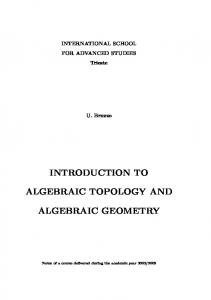
Let y - Yo = t{x - xo) be the line through that point with variable" slope t (see the figure)
(x, y)
•
The other, variable intersection point of the line and the curve (2) is obtained from the system " •
(t 2 - a).(x - xo) = (2axo + b) - 2Yot Y - Yo = t{x - xo) whose solution (x, y) depends rationally on t (for almost all t):
(2axo + b) - 2Yot x = Xo + 2 t -a y = Yo + t(x - xo)
Algebraic geometry (selected topics)
After substitution in the integral, one obtains rational function of argument t and the integral evaluates easily:
R(x, J ax 2 + bx + c)dx
=
R(x(t), y(t))x' (t)dt
= ...
Euler substitutions can be deduced from this general algorithm by different special choices of the point (xo, yo). Type Ill. The point (xo, Yo) = (A, 0) lies on the curve and we put y = t(x - A). Type II. The point (xo, Yo) = (0, VC) lies on the curve and we put y-.,fC = xt. Type 1. Here the situation is slightly more complicated. In the case a > 0 the curve (2) is a hyperbola with asymptotic directions (y'a, ±1). As starting point (xo, Yo), one takes the point at the infinity of one of these two directions. Then the .lines through that point are exactly the lines y = y'ax + t parallel to the asymptote. Each of these lines intersects the· curve in one more point (x, y) and we use y = y'ax + t. From previous discussion one can see that the expressibillty ofthe integral (1) in elementary functions is based on the following specific property of the conic (2). There exist rational functions x = ~(t)j Y = 1J(t) of one argument t such that for different parameter values t, the corresponding point (~(t), 1J(t)) lies on the curve. In this way one obtains all (but one) points of the curve. More specifically, for eacll' point (x, y) =F (xo, Yo) on the curve (2) it is sufficient to draw a line through (xo, Yo) with the slope t = (y-Yo)/(x-xo). We say that in such case curve (2) has rational parametrization. One can easily show that every plane curve of second order has a rational parametrization. Such curves have been called unicursal. Today one rather uses the term rational curves. Let us now apply the above principle of evaluation of the integral (1) with irrationalities of the type JP(x) where P(x) is a polynomial of degree greater than 2. In this case, along with the integral
(3)
R(x, JP(x))dx
one should consider the curve
(4) •
Here we have different behavior. . Some of the curves (4) do admit rational parametrization, and some of them do not. Examples. 1. It is obvious that the curve y2 = x 3 has rational parametriza:. tion (which one?).
2. The curve y2 = x 3 + x 2 also has rational parametrization x = t 2 - 1, y = t(t 2 - 1), It is obtained when one finds the intersection points of the curve and the lines y = tx through (0,0).
10
Aleksandar T. Lipkovski
. 3. The curve y2 = x 3 + ax 2 + bx + c has rational parametrization if and only. if the polynomial x 3 + ax 2 + bx + c has multiple root. When rational parametrization of the curve (4) exists, the integral (3) could be transformed into integral of rational function. How one evaluates the integral when there is no such parametrization? Interesting and complicated theory is obtained already when degree of the polynomial P(x) equals 3 or 4. It is sufficient to consider only the latter case, since degree 3 could be transformed to degree 4 by rational transformations. Example. For a given curve
(5) the right-hand side polynomial of degree 3 has at least one real root. Applying the translation along x axis one could make this root 0 i.e., one could put c O. After substitution y = tx we get
=
x+
a-t2
2
+b-
2
a- t 2
2
2
=0
The rational parametrization
(6)
,
•
a- t 2 x=u--2
a-t2
y=t ~-
2
transforms the curve (5) in the curve of degree 4 with equation 2
1
u = -t" - at
2
4
a2
+ 4 -
The parametrization (6) is rationally invertible
y t =-, x
u=
b
it has a rational inverse
a - (yjx)2
X
+ -"""'"'"'"'-'--'2
This is a very important fact, as we will see later.
2. Plane algebraic curves. Polynomials in many variables Now we should make the term "plane algebraic curve" more precise. Let K be field, so-called ground field, and K[x, y] polynomial ring in two variables with coefficients in K. , . Definition. Plane algebraic curve in the affine plane K2 = points in the plane defined by algebraic polynomial equation
x = {(x,y)
E
K21 f(x,y) = O}
Ak is the set of
'
Algebraic geometry (selected topics)
11
where I(x,y) E K[x,yj. This set is denoted X = V(J). Even such simple definition leads to several problems. Naturally, one would like to establish a one-to-one correspondence between sets and their equations. However, already in the real analytic geometry there exist examples where basically different equations define the same set, or equations define sets that seem unnatural to call "curves". So, in the real plane, equations x = 0 and x 2 = 0 define the x-axis, equations x 2 + y2 = 0, (x 2 + y2)2 = 0 and x 6 + y4 = 0 define the point (0,0), and equation x 2 + y2 + 1 = 0 defines the empty set. Immediately, two questions arise: first, how to treat objects which are produced by this definition but do not agree with our intuitive notion of "curve"; second, in which extent is the set X = V(J) determined by the polynomial I and how to modify the definition in order to get one-to-one correspondence. These problems are present already in the course of analytical geometry for first-year undergraduates. Problem with curves which "are not curves" is being bypassed by calling them "degenerate", etc. The question, in which extent is equation determined by the set of points, is usually not treated at all. The first problem can be easily solved: one should consider complex numbers instead of real ones. This is known as the complexification process. In the general case, one should take the algebraic closure of the given field. The "empty" curves like V(x 2 + y2 + 1) then disappear. In the sequel the ground field Kwill always be algebraically closed, unless the opposite is explicitly stated. Usually, it will be the field of complex numbers C. As to the second problem, it is being answered by the following fact, known as Study's lemma2 • Note that when polynomial I divides polynomial g, then 9 = Ih and every root of lis at the same time the root of g, that is V(J) C V(g). In the case of algebraically closed field the converse is also true. Lemma. Let K be algebraically closed field and I(x, y) E K[x, yj irreducible polynomial. H the polynomial g(x, y) E K[x, y) has a zero in every point of the curve X = V(J) (i.e., ifV(J) c V(g»), then I divides g.
Proof. Let 9 :f: 0 (in the opposite, I divides g). Then also I :f: O. If I is· constant, then I divides g. Suppose I is not constant, but an actual polynomial, say in y: I(x,y) = ao(x)yn + ... E (K[x])[yj with ao :f: 0, n > O. Let us show that 9 is then also an actual polynomial in y. If 9 = g(x) E K[xj, then 0 :f: aog = ao(x)g(x) E K[x) a.nd there should exist ~ E K such that ao(~)g(~) :f: O. Since K is algebraically closed, there exists 1] E K such that I(~, 1]) = 0, which is a contradiction to the choice of~. Therefore, g(x,y) = bo(x)ym + ... E (K[x])[yj with bo :f: 0, m > o. Let now R = R(J,g) E K[x) be the resultant of polynomials I and 9 with respect to y. Let ~ E K be such that ao(~) :f: O. Since K is algebraically closed, there exists 1] E K such that I(~, 1]) = O. Then also g(~, 1]) = 0 and therefore R(~) = O. In such way, aoR = 0 E K[x). Since ao :f: 0, it must be R = 0, which 2Eduard Study (1862-1930), German geometer (Fubini-Study metric in projective space)
12
Aleksandar T. Lipkovski
means that f and 9 have a nontrivial common factor. However, and therefore f must divide 9.
f
is irreducible
Corollary. Irreducible factors of curve's equation are determined uniquely (up to ordering). H f = pflp~2 ... p~. is a factorization in irreducible factors, then VU) = V(prlp~2 ., .p~.) = V(PIP2 ... Pk). This proof can easily be generalized for more than two variables. We see that in the case of algebraically closed field, one of all possible equations of a given curve is determined uniquely by the condition that it has no multiple factors i.e., it is reduced. Study's lemma is a special case of a very important theorem, which could be considered also as a generalization of the main theorem of algebra. It is a famous Hilbert's3 Nullstellensatz, which in its classical version states that "nontrivial" system of algebraic equations over an algebraically closed field always has a solution. Here "nontrivial" means that it is not possible to algebraically deduce a contradiction from the system. More precisely: IT the field Kis algebraically closed and ft, ... ,!k E K[Xl, . .• , xn] are polynomials in n variables such that there are no polynomials 91, ... ,9k E K[Xl, ... , xn] for which it would be 91ft + ... + 9kfk = 1, then the system of algebraic equations •
• • •
has a solution. . It is known that polynomial ring in one variable over a field is a PID (principal ideal domain): it is even Euclidean. This is a consequence of the existence of Euclidean gcd division algorithm. However, in polynomial rings in two variables this is no more true. For instance, ideal (x, y) cannot be generated by single polynomial. However, in 1868 Gordan4 proved that it is possible to find a finite generating set of polynomials in every ideal. His proof was constructive - he described a construction of such basis. Many mathematicians tried to generalize Gordan's construction to the case of more than two variables, but nobody could overcome computing difficulties, and for twenty years this problem, known as Gordan's prob1em, remained open. In 1888 Hilbert proved in his famous basis theorem that every ideal in the polynomial ring with n variables has a finite basis. His proof was existential, not constructive. It has been said that Gordan, after he saw Hilbert's proof, said: "Das ist nicht Mathematik. Das ist Theologie!"s. Only when later Hilbert folffid a constructive proof, Gordan was satisfied and said that theology has its merits. Only after this, existential proofs in mathematics became legitimate. 3David Hilbert (1862-1943), German mathematician. Most famous for his list of problems for 20. century 4Paul Albert Gordan (1837-1912), German mathematician 5 "This is not mathematics. This is theology!" •
13
Algebraic geometry (selected topics)
The notion of resultant was used in the proof of Study's lemma. Let us briefly describe it here. Let A be a UFD (unique factorization domain, factorial ring), say polynomial ring over a field, and let I, 9 E A[x] be two polynomials with coefficients in A, 1= aoxm + ... + am, 9 boxn + ... + bn (we allow also the possibility ao, bo 0). Since A[x] is also a UFD, we are interested in their common divisors. The definition of a common divisor easily leads to the following lemma.
=
=
Lemma. Polynomials I and 9 have nontrivial common divisor {:} there exist polynomials u, v E A[x], u, v '" 0 such that deg u < deg I, deg v < deg 9 and
vI = ug. V
If one writes this condition explicitly, one has u = cOx m - 1 = doxn - l + ... + d n - l and from equality vI,= ug one deduces m
n-l
n
+ .. , + Cm-I,
m-I
'"'" L...J aiXm-i . '"'" L...J djXn-J'-l - '"'" L...J bi Xn-i. ' '"'" L...J CjX m-J'-l = ... i=O j=O i=O j=O m+n-l
=
E E (aidj -
k=O
biCj)x(m+n-I)-k = 0
Hj=k
and comparing the coefficients for x one obtains system of m
E
(aidj-biCj) =0
+ n linear equations
(k=O, ... ,m+n-l)
i+j=k
or explicitly
=0 =0 • • •
••• • •
• • • • • • •
••• • •••• • •• •• •• •• ••• ••• ••
• • • •
•••••••
- blCm-1
aOdn - 1 - bn-1Co aldn - l - bnCo
=0 =0 =0
• • • • • • • • • • • • • • • • • • • • • • • • • • • • • • • • • • • • • • • • • • • • • • • • • • •
- bnCm-l = 0
with m+n indeterminates Co, ... Cm-l,do, ... ,dn - 1. This system has nontrivial solution if and only if its determinant equals O. Definition. Determinant of this system, i.e., the determinant " al
• • •
am
ao
al
• • •
am
n
•••
R(f,g) =
ao bo
bl
• • •
bn
bo
b1
• • •
al
•••
am
bn
m
•••
bo
b1
•••
bn
.
14
Aleksandar T. Lipkovski
is called resultant of polynomials !, 9 with respect to x. The resultant is a polynomial in coefficients ai and bj of degree m + n, homogeneous in each group of indeterminates. Preceding discussion proved the following theorem. Theorem. Polynomials! and 9 have nontrivial common divisor if an! only if R(f, g)
= O.
Applications. 1. Solution of systems with two polynomial equations. Let !, g E K[x, y] (K[x])[y] be two polynomials and R(f, g) R(x) E K[x]. H (xo, yo) is a solution of the system
=
=
,
!(x,y)
= 0,
g(x,y)
=0
then R(xo) = O. One consequence is, if the system has infinitely many solutions, then polynomials! and 9 have a nontrivial common divisor h = gcd(f, g) and the ideal (f,g) = (h) is principal. 2. Parameter elimination. Suppose curve X is described by its rational parametrization
x = Pl(t)/Ql(t) y = P2(t)/Q2(t) Let !(x, t) = Pl(t) - Ql(t)X, g(y, t) = P2(t) - Q2(t)y and let R be the resultant of these polynomials. Then .
(xo, Yo) E X {:} 3to : !(xo, to)
= R(f,g) E K[x, y]
= g(yO, to) = 0 {:} R(xo, Yo) = 0 •
This means that the equation of X is R(x, y) = O. Example. Find the equation of the curve that has a parametrization x = t 2 , Y = t 3 - t. Here f = t 2 - x, 9 = t 3 - t - y and
R(f,g)
=
1 0 0 1 0
0 1 0 0 1
-x
0
0 1 -1 0
-x
0 0
0
-x
-y
0
-1
-y
=y2 _ x 3 + 2X2 -
x I
Therefore, the equation of X is y2 = x 3 - 2X2 + x. One could obtain it also without use of the resultant, but the present method is generally applicable.
3. Transcendence degree. Hilbert's Nullstellensatz
!
Let K be a field and L its extension. Subset S c K is algebraically independent over K if there is no polynomial relation between elements in S, i.e., if there is no polynomial ! E K[Xl,'" ,xn ] such that ! (Cl, ... ,en) = 0 for some
--- - - -
-----
- ---
---
- ---
Algebraic geometry (selected topics)
15
Cl, . . . ,en E S. Family of algebraically independent sets is ordered by inclusion. Maximal elements of this family i.e., maximal algebraically independent sets are called transcendence bases of Lover K. For example, in the field of rational functions K(Xl, ... ,xn ) the set {Xl, ... ,Xn } is one of its transcendence bases over K. Note that, if S is a transcendence basis of Lover K, then L is algebraic over K(S). Main statements about transcendence bases are analogous to corresponding statements about (linear) bases in vector spaces over fields. Theorem. A. Let L be the field generated over K by the set M and let N c M be its algebraically independent subset. There exists a transcendence basis B between N and M. In other words, algebraically independent set can be extended to transcendence basis by adding elements from a given generating set. Theorem. B. Every two transcendence bases of the field Lover K have the same cardinality. Cardinality of any (and every) transcendence basis of Lover K is called transcendence degree of that field extension. Our next goal is to prove Hilbert's Nullstellensatz. That will be done in few steps. Step 1. Let K be algebraically closed and L its finitely generated extension. There exist elements Zl, . .. , Zd+1 in L such that 1. they generate Lover K, 2. Zl, ... , Zd are algebraically independent, 3. Zd+1 is algebraic over K(Zl, ... , Zd). Proof. Follows from the known theorem on the primitive element.
Step 2. Let K be algebraically closed field and Ft, ... , Fm E K[tl' ... , tnj polynomials. H the system of equations Fl = 0, ... , Fm = 0 has a solution in finitely generated extension Lover K, then it has a solution in K also. Proof. L is of the form L :::; K(Xl, ... ,Xr ,1]) where Xl,". ,Xr are algebraically independent over K and 1] is algebraic over' K(xt, ... ,xr ). Let F(xl, ... ,xr,y) E K(Xl, ... ,xr)[yj be the minimal polynomial of 1]. Let now (el, ... ,en) be the solution of the system in Ln. Onehasei =Ci(Xl, ... ,X r ,1]) for some polynomials Ci(xt, ... ,xr,y) E K(Xl, ... ,xr)[yj. Since F is minimal, there exist polynomials Qi such that
I
identically with respect to Xl, ... , Xn y. Since K is infinite, there exist elements al, ... ,an E K such that all denominators in coefficients of polynomials F,Ql' ... ,Qr,Cl , ... ,Cn E K(xt. ... ,xr)[yj and also the highest order coefficient of polynomial F are different from 0 after substitution Xi = ai. Since K is algebraically closed, there exists (3 E K such that F(al, ... , a r , (3) = O. Then 'Yi = Ci(al, ... , a r , (3) is the solution in Kn.
16
Aleksandar T. Lipkovski
Step 3. If polynomials F l , ... ,Fm E K[tl,'" ,tn ] do not generate the unit ideal, then the system Fl = 0, . " ,Fm = 0 has a solution in the field K. Proof. Ideal (Fl , ... ,Fm) is contained in some maximal ideal M. Therefore the quotient L = K[tl, ... ,tn]/M is a field. Let the image of ti in L be ~i' Obviously, L = K(6, ... ,~n) and (6, ... '~n) is a solution of our system in the field L. According to Step 2, there exists a solution in K. ,
Step 4. If the polynomial G equals zero in all zero-points in Kn of polynomials FI , ... ,Fm, then for some r, Gr E (FI , ... ,Fm). Proof. Introduce a new variable u and' consider polynomials FI , ... ,Fm' uG - 1 in the polynomial ring K[h, ... ,tn , u]. According to assumption, they do not have common roots in K, and therefore (Step 3) generate the unit ideal: there exist polynomials PI, ... ,Pm, Q E K[tt, ... ,tn , u] such that PIFI + ... + Pm Fm + Q(uG -1) 1. This identity remains true after the substitution u I/G. Eliminating the denominator, one obtains the necessary statement. This proves the Hilbert's Nullstellensatz.
=
=
4. Algebraic sets and polynomial ideals Definition of algebraic sets in higher dimensional space generalizes the notion of plane algebraic curves. Intuitively, algebraic set is a solution set of system of polynomial equations: If h, ... ,/m E K[xl, ... ,xn], the set V(h, .. · ,/m) = {x E Kn I h(x) = .. , = Im(x) = O} of solutions of the system h(x) = ... = Im(x) 0 is called algebraic set in the affine space Kn. For m 1 (one equation), the corresponding set V (f) is called hypersurface.
=
=
Even for plane algebraic curves it was not easy to establish a one-to-one correspondence between solution sets and equations: different equations could represent the same algebraic set. Instead of systems, let us consider their left-hand sides, that is, finite sets of polynomials. Instead of finite sets, it is useful to consider arbitrary sets of polynomials. . We shall use the notations A = K[XI' •.. ,xn ] for ground polynomial ring and X = Kn = Ai< for ambient affine point space in the whole section. Definition. For any subset S C K[XI"" ,xnJ, algebraic set in X defined by S is the set V(S) = {~= (~I'''' '~n) E X I'll E s, I(~) = O} eX. In this way one obtains the correspondence between subsets in A and subsets in X, that is, the mapping of partitive sets V : 1'(A) -+ 1'(X). Let us establish its elementary properties. _ Lemma 1. (a) SeT:::} V(T) c V(S) (more equations, less solutions).
(b) V(0) = X, V(A) = 0. (c) V(SI U S2) = V(SI) n V(S2)' (d) V (/1, ... ,Im) = V (h) n ... nV (fm) (every algebraic set is the intersection of hypersurfaces).
na
One can easily show that even for arbitrary unions V(Ua Sa) = V(Sa). Does the analogous statement hold for intersections, at least for finite ones?
17
Algebraic geometry (selected topics)
Lemma 2. If 1= (S) is the ideal generated by S
~
A, then V(S) = V(I).
=
According to the Hilbert basis theorem, the ring A is Noetherian, I (ft, ... ,fm) and V(S) V(I) V(ft, ... ,fm). Therefore, every set V(S) is algebraic set, described by finite set of equation.
=
=
One sees, that the mapping V defines (anti)epirnorphism of partially ordered sets
V : ideals inA
~
algebraic sets in X
•
•
When do the different ideals define the same algebraic set? Here the main role is played by the Hilbert's Nullstellensatz. It could be stated in the following manner: if V(I) =
0, then I = A
and its generalized form: if V(I)
=
c V(J), then f
E
.Jj
=
Here .Ji RadI {a E A 13r > 0: a r El} C A is the radical of the ideal I. Construction of radical of a given ideal is possible in every commutative ring and has the following main properties, which could be easily proved.
Lemma 3. (a) (d)
.Ji is ideal in Ai
(b) le J ~
.Ji c.JJ;
(c) I C
Vi;
J.Ji=Vi. Proposition. V(I) = V(J)
.Ji = .JJ
Proof. The direction - I corresponds to the closed set V (J) = W CV. Ideal J / I = I (W) /I(V) of algebraic subset W in algebraic set V is denoted by Iv(W). Therefore, here we also have the corresponding bijections
r
algebraic subsets in V {:} radical ideals in K[V] irreducible algebraic subsets in V {:} prime ideals in K[V] points in V {:} maximal ideals in K[V] The Zariski topology on V is induced from X = Kn. Its open base is also built by , principal open sets D(g) = V \ V(g), 9 E K[V]. Using regular functions one can define mappings which connect algebraic sets and play the role of morphisms in the corresponding category. Let U C Kn, V C Km be two algebraic sets and cp : U ~ V a mapping. Composition with cp defines a mapping
cp* : functions on V
~
functions on U
in the usual way, by the formula cp* (J) = f 0 cp. Definition. We say that cp is a regular mapping, if cp* transforms regular functions into regular functions, that is, if f E K[V] =? cp* (J) E K[U].
Proposition. (a) cp is a regular mapping {:} it is defined in coordinates with m regular functions, that is, there exist It, ... , fm E K[U] such that cp(x) = (Jt(x), ... ,fm(x» E V for all x E U. •
22
Aleksandar T. Lipkovski
(b) Hcp is regular, cp. : K[V] ~ K[U] is an algebra bomomorphism. (c) Conversely, for any algebra bomomorpbism h : K[V] ~ K[UJ tbere is a regular mapping cp : U ~ V such tbat cp. = h. (d) Tbe mapping U
~l
•
I
)
V K[V] is a contravariant functor. Tbe category of algebraic sets and regular mappings is equivalent to tbe category of finitely generated K-algebras witbout nilpotents (so called affine K -algebras) and bomomorpbisms. Proof. (a) H Yi E K[V] are coordinate functions (images of generators of polynomial ring in which the algebraic set V is defined) and cp·(Yi) = Ji E K[U], then for "Ix E U, i-th coordinate of the point cp(x) is Yi(cp(X» = CP·(Yi)(X) = Ji(x) and cp(x) = (ft (x), ... ,/m(x». Conversely, if cp is a mapping of that form and 9 E K[V] a regular function on V, then for "Ix E U, cp·(g)(x) = g(cp(x» = g(ft(x), ... ,/m(x» is a polynomial function of coordinates x, that is, a regular function. (b) is obvious. (c) Let again Yi E K[V] be coordinate functions and h(Yi) = li E K[UJ. Define for x E U, cp(x) = (ft(x), ... ,/m(x» and prove that cp(x) E V. Indeed, if F E I(V), then F(YI, ... ,Ym) = O. One has 0 = h(F(YI, •. ' ,Ym» = F(h(YI), ... , h(Ym» = F(ft, ... ,/m) and F(cp(x» = h(F)(x) = 0, and this means exactly that cp(x) E V. For x E U and 9 E K[V] one has cp. (g) (x) = g(cp(x» =
g(ft (x), ... , Im(x» = g(h(Yl)(X), ... , h(Ym)(x» = h(g)(x) i.e., cp. = h. (d) This is also straightforward. Definition. Isomorphism 01 algebraic sets 7 is isomorphism in the categorical sense, that is, a regular mapping which has inverse regular mapping. In this equivalence of categories, it corresponds to isomorphism of algebras, Le., U ~ V {:} K[UJ ~ K[V]. Examples. 1. Projection cp{x, y) = x is a regular mapping of the hyperbola V = {xy = I} in the line Ai, but not an isomorphism (not even a set bijection). Corresponding algebras are K[x,y]/(xy -1) ~ K[t]. 2. Mapping. cp : Al ~ V = {y2 = x 3 }, t t-+ (t 2 , t 3 ) is regular and a settheoretic bijection. However, it is not an isomorphism. The corresponding homomorphism of algebras cp. : K[V] = K[x, y]/(y 2 - x 3 ) -+ K[t] = K[Al] is defined by x t-+ t 2 , Y t-+ t 3 • Its image is Im cp. = K[t 2 , t 3 ] ~ K[t]. Since cp is a bijection, it has • • mverse mappmg y/x, (x,y) ~ (0,0) 1jJ: V -+ At, 1jJ(x,y) = 0, (x, y) = (0,0) 7 Biregular
isomorphism, as opposed to birational isomorphism which will be introduced
later. •
•
-_.
_
. .-
..
23
Algebraic geometry (selected topics) .
but it fails to be regular in the point (0,0). One could give the following informal interpretation. Algebra K[V] is smaller than K[AI], since in the latter there is a polynomial function with derivative in 0 different from 0, and in the former there is no such function: mapping is "leveling" all tangent vectors in O. 3. Parabola y = xk is isomorphic to the line Al. The corresponding isomorphisms are K(X1"" ,Xd) K{Ad) is algebraic. This extension defines a regular mapping V -7 Ad, so-called nONnalization of the algebraic set V. Normalization is a finite morphism, which means also that it is a finite covering, i.e., over each point of Ad there are at most d points of V. This gives us another geometrical expJanation of dimension.
=
Every local ring Oz.v (x E V) has the same dimension dim V. In local rings (rings with only one maximal ideal) there exists a connection between dimension and the maximal ideal itself: dimK M/ M2 2: Krulldim O. The ring Oz.v (and the point x) is regular, if the exact equality holds. What is the meaning of the vector space Mj M2? It consists of linear parts (Le., differentials) of all functions, regular and equal to zero in x. Therefore, its dual vector space "CM/ M2)* plays the role of the tangent space to the algebraic set V at the point x. The above inequality means that there can exist points which are not regular in the sense that the dimension of the tangent space is strictly greater than the dimension of V itself. Such points are special points. H V is defined by its global equations, they can be characterized in the following way. Definition. Point x E V is a singular point (singularity) of algebraic set V = VU1' ... ,fie) c An if it is a solution of the following system: •
hex)
of-
of-
= 0Xl• (x) = ... = 0 Xn• (x) = 0
(i = 1, ... ,k).
In other words, the singular points are the points where the rank of the Jacobi matrix (:!~ (x) ) ,:=1 •...• 1e drops down. In regular points this rank is equal to J=l •... n
codimension of V. The algebraic definition of singular point, independent of the embedding of V in ambient affine space, was introduced by Zariski8 • He also proVed equivalence with above traditional analytical definition. 80scar Zariski (1899-1986), italian and american algebraic geometer. ,
,
27
Algebraic geometry (selected topics)
••
Algebraic sets without singularities, nonsingular varieties, are the closest analogons of smooth manifolds or complex-analytic varieties. The presence of singular points complicates the structure of algebraic varieties and makes them interesting. Example. There are two typical plane singular cubics, which correspond to simplest types of singularities. These are the alpha-curve y2 = x3 + x2 with a nodal point (a "node"), and the semicubic parabola y2 = x3 with a cuspidal point (a "cusp"). The theory of singularities of algebraic varieties is a very deep theory, which itself requires a long introduction. There are many aspects of studying singularities, such as classification by discrete invariants, topological structure, resolution of singularities, etc. One fruitful method for investigation of singularities of hypersurfaces is given by a combinatorial-geometrical invariant called Newton polyhedron. It was introduced by Newton, but it attracted proper attention only recently, mainly in the work of Arnold's singularity group, in the 1970's (see [2]). Some simple, though interesting combinatorial connections between singularity and its Newton ' polyhedron were studied by the author [17].
6. Projectivization. Projective varieties Besides the algebraic closure of the ground field, there is one more problem in correspondence between the curve as a set of points on one side, and its equation on the other. IT the degree of the curve's equation is d, the number of intersection points with an arbitrary straight line is at most d, but it can also be less. Let C be a plain curve of degree d, defined by equation f(x,y) = 0 where f is a polynomial of degree d. IT L: x a + bt, y c + dt is a straight line, the intersection of C with L is determined by the equation
=
f(a+ bt,c+ dt)
=
= g(t) = ao(a,b,c,d)· t
d
+ ...
It can happen that some of the roots are multiple, that is, some intersections have higher order. The notion of intersection multiplicity resolves this problem (this, however, is not trivial). However, it can happen that the degree of the equation in t is strictly less than d, since the coefficient of the highest order term equals O. In the case of hyperbola and its asymptotic lines, the intersection point has "gone to infinity". Therefore, the points at the infinity should be introduced. It is done with the process of projectivization. There are many equivalent ways to define projective space. A common one is to define the n-dimensional projective space IPn over the field K as the set of all one-dimensional subspaces, that is, the set of all lines through the origin in the vector space Kn+l. IT one considers a unit sphere in this space, each line intersects the sphere exactly in two antipodal points. For this reason, in topology, IPn is defined mostly as the sphere sn C Kn+l with its antipodal points identified. We are interested in analytical approach to this construction: n-dimensional projective space IPn = 1P1< over K is the quotient of the set Kn+l \ {O} by the equivalence relation, induced by homothety: (Xo, Xl,' •. ,Xn ) "" (AXo, Axl,'" ,AXn )
28
Aleksandar T. Lipkovski
where A ",. O. Points in projective space are the corresponding equivalence classes, denoted x = (xo : Xl : ••• : xn). Therefore, (xo: Xl : ••• : Xn) = (AXo : AX1 : ... : AXn ). Numbers Xi are homogeneous coordinates of the point x. Since there is always a coordinate different from 0, the space pn is covered by sets Ai = {x E pn I Xi ",. O} = {x = (Xo: ... : ~: ... : xn)} ~ Kn, each of them isomorphic to the affine space • An. These are the affine charts of the projective space. The transition from homogeneous coordinates of the point X = (Xo: Xl: .•. : Xn) in pn to coordinates (l:xl/xo: ... :xnlxo) ~ (xl/xo, ... ,xnlxo) in the affine chart A8 ~ An is called dehomogenization in Xo, and the converse transition from coordinates (Y1,'" ,Yn) in An to coordinates (1: Y1 : ... : Yn) in pn homogenization.. The complements of affine charts pn \
Af
= {x E pn I Xi = O} = {x = (xo : '" :
9:... : Xn)}
=
P?-l ~ pn-1 are isomorphic to the projective space of dimension n - 1, that is pn= Ai U Pf-1. This decomposition is easily seen on the previous model also. If in the space K n+1 one considers the i-th coor-dinate hyperplane Xi: Xi = 0 and its parallel hyperplane Yi : Xi = 1, then one could divide the lines through the origin into two types: the lines which intersect hyperpl~e Yi and the lines which are parallel to it. Lines in the first family correspond to points of this hyperplane, and they form an affine space Yi ~ K n = An. The other family of lines is the set of all one-dimensional subspaces of the vector space Xi ~ Kn. They form a projective space pn-1 of dimension n - 1. Points in this projective space, that is, lines in Xi, represent the "points at infinity" of the corresponding parallel lines in the "finite" part Yi. The whole projective space pn is the (disjoint) union of its "finite" part Yi ~ An and its "points at infinity" complement' pn-1. Note that the distinction between finite points and points at infinity of the space pn is only formal, since it depends on coordinates. Every point could be made finite or infinite by corresponding change of coordinates. The next step is to define algebraic subsets in projective space. How. ever, there is a small difference comparing to affine case. Polynomial equations in homogeneous coordinates in pn can always be considered to be homogeneous. If 1 E K[so, Sl, .. , ,sn] is a polynomial over K in n + 1 indeterminates so, Sl,'" ,Sn, then it is represented as a sum of its homogeneous components 1 = 10+ h + ... + Ir. If now ~ = (~o: ~1 : ... : ~n) is a point in pn for which I(~) = 0, r then I(A~O,' .. ,A~n) = lo(~o, . .. ,~n) + Ah (~o, ... ,~n) + ... + A Ir(~o, . .. '~n) = 0 for all A E K*. Since the field K is infinite, it follows that all li(~O, .. . '~n) = O. The transition from homogeneous polynomial I(so, ... ,sn) E K[so, ... ,sn] to polynomial 1(1, t1l'" ,tn ) E K[h, ... ,tn ] is called dehomogenization, and the transition from polynomial g(t l , ••. ,tn ) E K[t1l'" ,tn ] to homogeneous polynomial s~egg ·g(s11 so, ... ,snl so) E K[so, S1l .. ' ,sn] (this is a homogeneous polynomial!) homogenization ·with respect to so. Closed algebraic set V c pn is the set of common zeros of the finite (or infinite) set of polynomials 1 E K[so, ... ,Sn]' The correspondence between closed sets V and ideals I is the same as in the affine case, only the ideals obtained are not arbitrary, but with every polynomial they contain also all its homogeneous
-i
•
Algebraic geometry (selected topics)
29
components. Definition. Ideal I C K[so, . .. ,sn] is homogeneous if: f El::} all homogeneous components of f belong to I. Every homogeneous ideal has a basis of homogeneous polynomials. Therefore, every closed set in projective space can be defined by homogeneous equations. Another difference is the absence of Hilbert's Nullstellensatz: there are homogeneous ideals defining the empty set. They can be easily described.
= 0 {:} for soine k, I::> I" := (so, ... ,sn)". Proof. The direction - X~ the mapping I
=
u·o -- v m,O, ... ,0 Ul
=
Vm-l,l, .•. ,0
•••
Un
=
Vm-l,O, ... ,1
is regular and inverse for V~ : lP'n -t lP'd;:' -1. So, V~ : lP'n E:! V~ (lP'n) = V,.:: C lP'd;:' -1. The dimension of the Veronese variety V,.:: is n. Example 1. For n = 1, m = 3, VJ : lP'1 0), forms Fi define subvarieties Gi and let F = F{'l ... F;:· be the corresponding product. Then (F) n1(F1) + ... + nk(Fk) D (more precisely, this holds in affine chart). In other words, ea.c4 effective divisor on pn is a divisor of a homogeneous polynomial form. Let now D be an arbitrary divisor, D = D1 - D2 its decomposition as difference of effective divisol"s, and Di (Gi) (i 1,2) their representation by homogeneous forms. Let c4 degDi and d degD d1 - d2 • Consider the rational function f = GI/xgG2 and its principal divisor (J). This is a global rational function of degree 0, that is, an element of the field K(pn). Its principal divisor is (J) + dH = D1 - D2 = D, where H is the divisor of the . hyperplane Xo = 0 (the hyperplane section divisor). This means that D ,.., dH and CI(pn) = Z . H ~ Z.
=
=
=
=
=
=
=
= =
Theorem. [31, p. 176] Let X be a nonsingular variety, Y C X its subvariety
and U = X \ Y. Then (1) the mapping ,£niGi ~ ,£ni(Gi nU) is an epimorpbism Cl(X) ~ CI(U)j (2) ifcodimx Y ~ 2, then it is an isomorphism CI(X) 9!! CI(U)j (3) if codimx Y = I, then 1 1-+ 1 . Y defines a mapping Z ~ CI(X) and the sequence Z ~ CI(X) ~ CI(U) ~ 0 is exact. Example. IT Y C p2 is an irreducible curve of degree d, then CI(P2 \ Y) 9!! Zd. This can be easily proved i?y the previous theorem.
10. The divisor class group of nonsingular quadric and cone Let us now determine the divisor class group of the nonsingular quadric Q. We shall represent the quadric by the so-called Segre embedding 14 • Stop for the moment to define the product of varieties. The set-theoretic (Cartesian) product of affine spaces is again an affine space: An X Am = An+m, and similarly for corresponding closed subsets. However, for projective closed sets, the situation is more corp.plex. How should one define a structure of a projective variety on the set-theoretic product of two projective lines? Define the Segre embedding S:]p1 X pI ~ p3, (XO:X1) X (YO:Y1) ~ (.zoO:ZOl:ZIO:Z11) with Zij = XiYj. Th~ image S(P1 X pI) is on the quadric Q {zoozu ZOlZlO} C p3. Conversely, if the point (zoo: ZOl : ZIO: Zll) E Q, then at least one coordinate, say zoo =F 0, and S «zoo: zot} X (zoo: ZIO» (ZooZoo: ZOOZOl : ZOOZ10: ZOl ZIO) (zoo: ZOl : Z10: Zll). So, the mapping S defines bijection pI X pI ~ Q, which makes it possible to transport the structure of algebraic variety, induced on the quadric Q from the ambient space p3, on the set pI X PI. Could one define this structure independently from the embedding? Homogeneous polynomial on Q has the form F(zoo, ZOl, ZIO, Zll) = F(xoYo, XOYb XIYO, X1yt} = G(xo, Xl; Yo, Y1). This is a polynomial in two groups of variables, homogeneous in each group separately. The degree in each of the groups of variables need not to be equal: if s = degy G < degz G = r, then the equation
=
=
"
=
=
14Corrado Segre (1863-1924), Italian geometer, famous by his work in birational geometry.
44
Aleksandar T. Lipkovski
G = 0 is equivalent to the system y~-BG = yr-BG = O. Closed subsets ·in pl x pl are defined by systems of polynomial equations of the form G(xo, Xl i Yo, Yl) = 0, homogeneous in each group of variables separately. Subvarieties of codimension 1 in pl X pl are defined by one such equation, as in standard projective space. Namely, if the polynomial F(XO,Xliyo,Yl) is homogeneous in each group of variables separately, and if F factorizes in product of two polynomials F = G . H, then each of the factors must have the same homogeneity property. Let us determine the divisor class group CI(pl x pl). The given divisor D E DiV(pl X pl), in addition to the usual degree degD, has two degrees deg z D and degll D in each of the groups of variables, and one has deg D = degz D + degll D. In this way, one obtains an epimorphism Div(pl x pl) -+ Z2, D t-+ (degzD,degIlD). It is straightforward to check that its kernel is exactly the principal divisor subgroup, so CI(Pl x pl) ~ 'I}. The pair (deg z D, deg ll D) is called type of the divisor D. Segre embedding S : pl X pl -+ p3 defines a homomorphism Div(p3) -+ Div(Pl X pl) by intersection with Q. It extends to classes of divisors, and coincides with the diagonal embedding CI(P3) = Z -+ Z2 = CI(Pl X pl), 1 t-+ (1,1). Example. Apply this to the case of the projective space cubic C. It has the following parametrization: Zll
=
V
3
Obviously, C c Q. Is it possible to represent C as intersection of the quadric and some surface? Consider the cone K : ZOlZll = z~o. The intersection is KnQ = LUC where L is a line. The divisor class group is CI(P3) = Z· H ~ Z where H is the divisor of the (hyper)plane section, so K ,..., 2H. The diagonal ~mbedding gives K = 2 t-+ 2(1,1) = (2,2) = K n Q. The type of this divisor is K n Q = L + C = (2,2), and the type of the divisor L = (1,0). Therefore, one has the type of C = (2,2) - (1,0) = (1,2). Let now Y C p3 be the surface such that its intersection with the quadric is Y n Q = C. Then the type of the divisor Y n Q is, on one side, rC = r(1,2) = (r,2r) and on the other, dH = d(l, 1) = (d, d). Since (r,2r) :f. (d, d), this means that the answer to the above question is negative: there is no surface which would intersect the quadric Q by the curve C! Consider the cone X = V(xy - z2) C A3, with ideal [ = [(X) = (xy - z2) C K[x, y, z} and coordinate ring K[X] = K[x, y, z]J(xy- z 2), and determine its divisor class group. The generators of the ring, the images of the indeterminates X, y, Z we will denote also x, y, z. The directrisse of the cone is the line Y = V (y, z) C X C A3, and this is an irreducible subvariety in X of codiniension 1 - a simple divisor in X. Corresponding chain ofideals in K[x,y,z] is
(0) C (xy - Z2) c (y,z) c (x,y,z) However, after the factorization by [(X) one obtains the ideal [x(Y) = (y,z) c K[X], which is of height 1 but not principal! The corresponding chain of ideals is (0) C (xy - z2) C (y, z) C (x, y, z)
45
Algebraic geometry (selected topics)
H (y, z) = (f) in K[X], then the corresponding originals in K[x, y, z] would satisfy y, z E (f, xy - z2), J E (y, z, xy - z2) = (y, z), and this gives a contradiction when one considers J modulo ideal (x, y, z)2 (that is, its linear components). So, Y '" 0 in Cl(X)! Let us prove that 2Y = 0 in Cl(X), or that 2Y is principal. Consider the function yE K[X], and find a local equation of the set V(y) n X = Y in the open subset U D(x)nX. Then K[U] K[x,y,z,x- I ]/(xY- Z 2) K[x,x-l,z], y X-I z2. One has Y n U = V(y, z) n U, the corresponding coordinate ring is K[Y n U] K[x,x- l ,z]/(X- 1z 2,Z) K[x,x-l,z]/(z). The local equation of Y in U is z 0, the local parameter z. The function y E K[U] has the fOIm y X-I z2. Therefore v(y) = 2 and the principal divisor is (y) = 2Y. Now, there is the exact sequence Z -+ Cl(X) --t Cl(X \ Y) --t 0, where the first mapping is 1 t-+ 1 . Y . The ring K[X \ Y] K[X n D(y)] K[y,y-t,z] is factorial, so Cl (X \ Y) o. Therefore Z --t Cl(X) is an epimorphism and Cl (X) Z/2Z Z2.
=
=
= =
•
=
=
=
=
=
=
=
=
=
11. Group of points of nonsingular cubic. Elliptic curves As we have seen, the degree of the divisor defines a natural homomorphism of the divisor group on the group of integers Div(X) --t Z. In some cases it factors through principal divisors (that is, the principal divisors have degree 0) and defines epimorphism CI(X) --t Z. This was the case for projective space. This is also the case for nonsingular projective curves. Theorem. [33, t. 1, pp. 205-209] H X is a nonsingular projective curve, the degree of any principal divisor is O. The kernel Clo(X) of deg : Cl(X) --t Z is an important subgroup in Cl(X): Theorem. The following statements are equivalent: (1) the curve X is rational;
(2) the group Clo(X) = 0, that is, Cl(X) !:!! Zj (3) there exist two different points P, Q E X such that P '" Q. Proof. H Clo(X) = 0, each divisor of degree 0 is principal, and for any two different points P, Q E X there is a nonconstant rational function J E K(X) such that P - Q = (f). This function defines a rational mapping
1. Then D = D' + P, degD' = degD - 1, D' > O. By induction D' '" P + l . O. Then D '" P + Q + l· O. Find the point R such that
46
Aleksandar T. Lipkovski
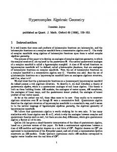
P + Q ,.... R + O. We do this by a geometrical construction. Suppose that points P and Q are different, and let p be the line that they determine. Let S be the third point of intersection of that line and the cubic X. Let q be the line through 0 and S and let R be the third intersection point of the line q and cubic X. Then one has P + Q + S ,.... (p) ,.... (q) ,.... 0 + S + Rand P + Q ,.... R + 0 (se the figure). In the case when some points coincide (P = Q or 0 = S), one takes tangents instead of secants p and q.
P
p
°
We have proved that any effective divisor D > on X is equivalent to the divisor of the form P + kO, where 0 is a fixed point. Obviously, k deg D - 1. If now D is a divisor of degree 0, then it is a difference of two effective divisors of the same degree D = Dl - D2 ,.... (R + k ·0) - (Q + k· 0) = R - Q. Using the same geometrical construction as above in reverse order, one finds the point S as intersection of X and the line through Rand 0, and then point P as intersection of the line through Q and S (see the same figure). One obtains P + Q,.... R+ 0 or D,.... R - Q,.... P - 0 Cp. Therefore, the mapping P t-+ Gp is bijective.
=
=
This bijection introduces a structure of an Abelian group on the set of points of the curve X. This structure is defined purely geometrically, by the constructions described above. The point 0 is the neutral element. If P and Q are two points of our curve, the point R is their sum, and S = - R. One could prove directly that this is a group. The most complicated part is the proof of associative law, elementary but long. How many nonisomorphic nonsingular cubics do exist? We shall give the answer to this question for complex ground field C. The equation of the plane nonsingular cubic is y2 = P3(X) where the right-hand-side polynomial of the third degree does nQthave multiple roots. By translation and homothety in x one could obtain two of its three roots to be and 1. In other words, P3(X) = x(x -l)(x - A) where the third root A =f:. 0,1 parametrizes all such curves. However, for different = x(x -l)(x + 1) and parameter values one could get isomorphic curves: curves y2 = x(x - l)(x - 2) are obviously isomorphic by isomorphism x t-+ 1- x.
°
y2
The three element permutation group S3 (with six permutations) acts on the root triple (0,1, A). If we apply the linear transformation on x again after permutation, to obtain the root triple (0,1, >'), it is easy to check that A could take 1 - A, l~A' A: l' A~ l. It follows directly one of the following six values: A, that all six curves which correspond to these parameter values are isomorphic. Let us produce a function in A, invariant with respect to this action and in this way
:t.
47
Algebraic geometry (selected topics)
remove the six-ply ambiguity. An obvious candidate would be
and another
(A i:-
Definition. IT X is anonsingular cubic with the equation y2 = x(x-l)(x-A) 0,1), the complex number
is called the j-invariant of the curve X. The function A t-t j(X) defines a siX-to-one covering j : Al -+ Al,
{A, :t.l - A, l~~' ~:l' ~il} t-t j(X), branched over points 0 and 1. The value of the j-invariant classifies nonsingular cubics, as the following theorem shows. Theorem. [15, p. 249], [31], ... a) Two cubics X are Y isomorphic {:} j(X) =
j(Y). b) For any complex number a there is a curve X with j(X) = a. Therefore, nonisomorphic nonsingular cubics are parametrized by points of complex line. Nonsingular cubics are called also elliptic curves. This name originates from elliptic integrals. When the arc length of the ellipse (and other curves) is being _calculated, the integrals of functions with radicals P4(X) appear. In the spirit of lecture 1, these integrals are connected to curves y2 = P4(X), which are birationally isomorphic to nonsingular cubics.
V
Classical theory of elliptic integrals culminated in the middle of the last century in the works of Legendre [15]. He reduced all elliptic integrals to the folrp lowing three basic types: first type F(cp) = !co . , second type E(cp) = 2 sm z
Jri Vl-
k2
2
sin xdx and third type G(cp) =
Jri (sm. z-c)
10 2
_
.sm
2
z
The arc length
of the ellipse is expressed by the elliptic integral of the second type, and the first type appears in the arc length of the lemniscate. There is a famil)!- of curves with this property, discovered by Serret [28], which is connected to so~e interesting questions of the theory of elliptic curves and arithmetic. For more details see [23],
[18].
48
AlekBandar T. Lipkovski
As we have seen, the set of points of elliptic curve forms an Abelian group. What is this group? Theorem. As a group, the elliptic curve X is a two-dimensional torus: X ~ CIA ~ JR/Z x JR/Z. Here A c C is a lattice, that is, a free additive subgroup A = Z + ZT C C of rank 2 over Z (T fJ. IR). Proof. [31, pp. 414-416] We will sketch the proof. It requires some classical theory of complex functions. Definition. The function p(z) =
~+
2: [(.z!w)2 - ~]
of the complex
w€A\{O}
argument z is called Weierstrass function. The Weierstrass function and its derivative p'(z) = - 2:w€A (.z':wl s are doubly periodic complex functions with periods 1 and T, in other words A-periodic functions. They satisfy the equation (p')2 = 4 p 3 - 92P - 93 where coefficients g2 = 60 2: w- 4 and 93 = 140 2: w- 6 , and the discriminant a = 9~ - 279i :f. o. w€A\{O}
w€A\{O} •
It follows from these properties that if the lattice A is given, then the mapping C -t jp'2(C) defined with z J-7 (p(z), p'(z)) factors through homomorphism C -t Cl A and induces a bijection of the torus Cl L and the cubic y2 = 4x3 - 92X - 93. Conversely, if the cubic is given, that is, two numbers 92 and 93 satisfying 6 = 9~ - 279i :f. 0, then one coUld show the existence of the lattice A such that its Weierstrass function satisfies the given equation. One could obtain also the connection between i-invarjant of the curve and its coefficients: J = 9i! 6 or i(X) = 17289va. Any lattice A or a complex number T fJ. lR defines an elliptic curve. Obviously, different values of T could define isomorphic curves, exactly when their i-invariants coincide. The following theorem describes when this takes place. Theorem. [31, p. 416] J(T) = J(T') {:} T' = ~;t: for some regular integer matrix (::) E G~ (Z) In the sequel we shall show the connection between elliptic curves and number theory. •
Let X be an elliptic curve with fixed origin 0 and corresponding group structure. For any n E N one has the mapping!pn : X -t X, P J-7 nP with !Pn(O) = O. One could show that this is a regular (polynomial) morphism and homomorphism of the group structure. .
Definition. Endomorphism of the elliptic curve with fixed origin (X, 0) is algebraic morphism f: X -t X which maps the point 0 again in O. H f and 9 are two endomorphisms, define their sum in a usual way, pointwise (f + 9)(P) = f(P) + g(P), and their product as composition (f. g)(P) = f (g(P». The zero-element will be the constant function O(P) = 0, the neutral element the identity l(P) = P. ,
Algebraic geometry (selected topics)
49
Lemma. Endomorphism of elliptic curve is a homomorphism of its group structure. The set End(X, 0) of all endomorphisms is a ring. Theorem. [31, p. 417], [15, p. 18] There exists a bijection between endomorphisms of the elliptic curve (X,O) and complex numbers a E C which leave the lattice invariant aA C A. In such way, an embedding is defined. Proof. From the Serre's theorem on isomorphism of algebraic and analytical structures on complex algebraic varieties [27], algebraic morphisms f : X -t X correspond to holomorphic morphisms f : Cl A -t CIA. Each such mapping extends to the mapping / : C -t C, /(A) C A. It is a holomorphic homomorphism in tp.e neighborhood of 0, so /(z) ao + alZ t a2z2 + ... and /(Zl + Z2) /(Zl) + /(Z2)' Comparing the coefficients in the equality ao + al(zl + Z2) + a2(zl + Z2)2 + '" = (ao+alzl +a2z~+'" )+(aO+alz2+a2z~+''') one obtains ao = a2 aa = ... 0 and /(z) = alZ. So, End(X,O) = R = {a E C1aA C A} is a ring, Z eRe C. Let us now analyze more closely rings of the form R = {a E ClaA C A} where A = Z + Zr (r ft JR.) is a given lattice. Note that ReA, RA c A, that is, the lattice A is a R-module.
=
= =
=
Lemma. Each a E R is integral algebraic number, and R is a subring of the ring of integral algebraic numbers O. Proof. aA C A {:} a . 1 = a + br, a· r = c + dr where a, b, c, d are integers. Therefore, (a - a)(d - a) - ·bc 0 and a 2 - (a + d)a + (ad - be) O. Clearly, integers do leave any lattice invariant, or Z C R. When does the lattice admit nontrivial endomorphisms?
=
=
Lemma. The ring R is strictly greater than the ring of integers Z {:} r is algebraic number of degree 2 over Q. Proof. One has: 3a E R, a ft. Z, aA C A {:} 3a, b, c, d E Z, b =F 0 such that a·1 a+br, a·r c+dr, and by elimination of a one obtains br2+(a-d)r-c O. Conversely, if rE Q(v'-D) = Q[v'-D] for some DE Z, D > 0, r = r + s';-D, then
=
=
R
=
= {a = a + br I ar =
2 ar + br EL}
=
2 {a + br ELl br EL}
= {a + br I a, b, 2br, b(r2 + DS2) E Z} since br2 = -b(r 2 + DS2)
+ 2brr.
It is clear that R is strictly greater than Z.
=
=
=
=
One has ReO OnK where the field K Q(r) Q[r] Q[v'-D], and is its ring of integers. Note that the lattice A is a projective R-module, since R®Q L®Q Q[r]. One has rankz R dimQ R®Q ;;:: rankz 2. This means that for some p E 0, = Z + Zp. Then Rn Zp is a subgroup in Zp, necessary of the form Rn Zp = c . Zp for some positive integer c E N.
°
=
=
°
=
°=
Lemma. (& definition) R = Z + c· Zp. The number c is called the conductor of the ring R.
I
50
Aleksandar T. Lipkovski
=
Proof. If x a + bp E R, then bp.= x - a ERn Zp c I b and x = a + c . b' p.
= c· Zp. In other words,
•
Example. Let D = 1, K = Q(i) = Q[ij and 0 = Z[ij = Z + Zi.
= i, then R = 0 = Z[ij, c = 1 and R = Z + Zi. 2. Ift = 2i, then R = Z[2ij ~ 0, c = 2 and R = Z+2Zi = {a + 2bi I a, bE Z}. 1. If t
,
,
Let us return to elliptic curves. Integers correspond to "trivial" endomorphisms I{Jn : X --+ X, P I-t nP. Is it possible to describe all elliptic curves which allow also nontrivial endomorphisms? The answer is given by a wonderful theorem of number theory. Definition. The elliptic curve X = tion, if End(X, 0) i: Z.
Cl A is a curve with
complex multiplica-
Theorem. (Weber, Filter, Serre) If the curve X has complex multiplication, End(X,O) its ring of endomorphisms and K Q[v'-Dj corresponding field R of algebraic numbers, then
=
=
(1) the invariant j = j(X) is an integral algebraic number; (2) Galois' group Gal(K(j)1 K) is Abe1ian, of order \Pic(R) I = ICI(R)\; (3) number j is rational {:} K(j) = K {:} ICI(R)I = 1 {:} ring 0 is factorial, and there are exactly 13 such values for j: D (discriminant) 1 2
•
c (conductor) 1 •
.
.
J
(invariant)
26 33 26 53
o
3 7 11
_33 53
19
_215 33
43 67 163
~2183353
1
_2 15
_2153353113 -2183353233293 2
3 7 3
2333113 24 33 53 3353173
3
The groups CI(R) and Pic(R) which appear in the theorem are the class group of fractional ideals of the ring R, and the class group of projective R-modules of rank 1. The question how many factorial rings 0 exist, has been answered only recently. From classical theoretical considerations it followed that there are at most o
51
Algebraic geometry (selected topics)
ten, and the calculated tables for small values of D conta.ined only nine such rings (the above table with conductor 1). It was a long-standing open problem whether there is tenth ring (the so called problem 01 the tenth discriminant). In 1967 Stark [29] answered negatively and showed that there is no such ring (see [12, p. 438], [3, p. 253]). .
12. Cartier divisors and group of points of singular cubic The notion of Weil divisor was introduced only for varieties that are nonsingular in codimension 1. In the case of curves, these are the nonsingular projective curves. But what about singular varieties? It would be possible to define divisors for arbitrary varieties as formal finite combinations D = :E niCi of irreducible subvarieties of codimension 1. However, already the notion of principal divisor (and the divisor class group) does not work: the multiplicity of a rational function can not be always consistently defined along subvariety of co dimension 1, since it may contain singular points. In this case one uses a different definition of divisor, suggested by connection between divisors and functions in projective space. The notion of divisor occurs as the answer to a classical question: is there a rational function that has zeros (ni > 0) and poles (ni < 0) of given multiplicity ni on given hypersurfaces Ci. If D = :Ei niCi is a divisor on JP'n, each irreducible subvariety Ci of codimension 1 is globally defined by one polynomial homogeneous irreducible equation gj = 0 and the solution of the problem is the rational function 1 = gfi. This is a global rational function on JP'n only if the degree of the divisor equals 0, that is, if :Eini = O. However, in any affine chart U; = {x;¥: O} it defines a proper rational function f; = f!xjEn i ). Inaddition, the family {U;, f;} (j = 0, ... , n) has the property that functions f; /Ik have neither zeros nor poles on intersections U; n Uk, since corresponding factors cancellate.
n
For arbitrary nonsingular variety X, in an analogous way, each Weil divisor D = :E niCi on X defines a family {U;, f;} consisting of covering U; of X and of rational functions f; E K(U;)* on each element of the covering, such that function f; on U; cuts out the principal divisor (/;) = D n U;, and rational functions I; / Ik have neither zeros nor poles on intersections Uj n Uk. One needs nonsingularity in order to describe each Ci locally by one equation gi = O. Such a family {U;, I;} is called coherent system 01 functions. Conversely, coherent system of functions {U;, f;} on X defines a divisor D = :EniCi on X: note that K(U;) is the field of fractions of the factorial domain K[U;] and represent f; in the form I; = g':t. The coherency conditions uniquely determine subvarieties Ci and multiplicities ni. Two coherent systems of functions {U;, I;} and {Vk, gd define the same divisor if and only if corresponding principal divisors coincide: (/j) = (gk) on intersections U; n Vk, that is, if rational functions f; / gk have neither zeros nor poles on U; n Vk • This defines equivalence on the family of coherent systems of functions. Corresponding equivalence classes are c~ed locally principal (or eartier divisors. ~. Weil divisor corresponds to each Carlier divisor and vice versa, and this is a bijection.
n
,'.,
52
Aleksandar T. Lipkovski
The good property of Cartier divisors is that they can be defined for arbitrary variety X, even when Well divisors can not. The product of two Cartier divisors {Uj, f;} and {Vk, gk} is a Cartier divisor {Uj n Vk, !;gk}, and this defines a group structure on the set CaDiv(X) of Cartier divisors. Analogously to Well divisors, this operation is written additively and called the snm. Every global rational function 1 on X defines a principal eartier divisor {X, J}. This defines a homomorphism K(X)* ~ CaDiv(X). The quotient group of Ca Div(X) by the subgroup of principal divisors is the group of Cartier divisor classes Ca CI(X) . .
IT the variety X is nonsingular in codimension1, then there exist both Well and Cartier divisors .. The construction of Well divisor, corresponding to Cartier one, defines a homomorphism CaCI(X) ~ CI(X). The construction of Carlier divisor shows that this is an inclusion. However, it does not have to be a surjection, as the example of the simple cone shows. In this case, the group CI(X) = Z2 is generated by the class of the directrisse L of the cone. This directrisse can not be defined by one equation in anyneighborhood of cone's vertex, since any function which should describe L as a set of points, cuts out the divisor 2L. Therefore, L is not locally principal, every locally principal divisor is principal, and Ca CI(X) = o. Let us now calculate the Carlier divisor class group of the singular cubic X = V(y2 z - x 3 ) C 1P'2 (the "cusp"-curve). That will introduce group structure on its set of nonsingular points, exactly as in the case of nonsingular cubic. Our construction follows that of [31, p. 187]. First prove an important lemma.
Lemma. (''removing the point from divisor's support" ; (generalization see in [33, t.· 1, p. 193]). If X is a plane projective curve, P E X its point and D E Ca Div(X) Cartier divisor on X, tben tbere is a divisor D' ,..., D wbose support does not contain tbe given point.
,
Proof. Let U be a neighborhood of P and 1 rational function defining locally principal divisor D in that neighborhood. Suppose that the support of the divisor contains the given point. This means that P is a zero or a pole of the function 1, of some mUltiplicity n. Take a global rational function 9 E K(X) which in the point P has zero or pole of multiplicity n. The divisor D' = D - (g) has the reqnired property, since the function 19- 1 is regular in some neighborhood of P. Let now X =V(y2 z - x 3 ) C 1P'2 with singular point S = (0:0:1) and let y = X \ S be the nonsingular subvariety. Each Cartier divisor D E CaDiv(X) is equivalent to divisor D' whose support does not contain the point S, that is, whose local equation does not have a pole in that point. Therefore, D' is a Weil divisor on Y. IT D is principal, D' is such. The divisor D' has not to be uniquely determined, but its degree is. In such way, one defines the degree of divisor D, that is, a homomorphism Ca CI(X) ~ Z. Consider its subgroup Ca CI(X)O of divisor classes of degree 0 and, as in the case of nonsingular cubic, define a mapping
=
=
=
=
f AA:-d ~ AA:
.
of degree d. From the exact sequence 0 --+ --+ [AI(f)]A: --+ 0 one has dim[AI(f)]A: = (A:!n) _ (A:-:+n) and PM(t) = e~n) _ (t+~-d) = d. (!":11)! + .... 3) Particularly, for n = 2, that is, for plane projective algebraic curves of degree d one has PM(t) = (t12) - (t+;-d) = d· t + (1- (d-1Yd-2». Note that if f E Q[t] is a rational polynomial of degree n such that in n + 1 consequent integer points k, k + 1, .. , ,k + n E Z it has integer values, then it can be written in the form pet) = a n (!) +an-l (n:l) + .. '+ao with integer coefficients. Therefore, the highest order coefficient of the Hilbert polynomial has the form din! (d E Z), which can be guessed from previous examples. Examples also show that the degree of Hilbert polynomial equals the dimension of projective variety X. This is really so. One can show that not only the degree, but also the whole polynomial (all its coefficients) is an invariant of the variety, independent from the embedding X C pn. Some of the coefficients· (the first and the last) have a special meaning and geometrical interpretation. Definition. Let Px(t) = d· r. + ... + Px(O). The coefficientd is called degree of projective variety X. The integer Pa(X) := (-IY[Px(O) - 1] is called arithmetical genus of the variety X. Example. Arithmetical genus of the plane algebraic nonsingular curve of degree d equals (d - 1)(d - 2)/2. One can see that the definition of arithmetical genus really does not depend on the embedding X C pn when it is expressed in terms of structure sheaf of the variety. Namely, if ~ is a sheaf on X, its Euler characteristic is defined by x(~) dimHO(X,~) - dimHl(X,~) + .... One could prove that Euler characteristic of the structure sheaf 0 of regular functions on a variety X equals X(O) = Px(O). Therefore, the arithmetic genus of nonsingular projective variety X C pn equals Pa(X) = (-1Y[x(0) -11 where r = dimX. For curves this is reduced to equality Pa(X) dim Hl(X, 0) hl(X, 0).
r;.
=
=
=
Algebraic geometry (selected topics)
61
14.3. Geometrical genus of projective variety. The notion of geometrical genus appears for the first time in the works of Riemann, connected with maximal number of linearly independent global differential forms on a Riemann surface. On the language of sheaves this can be expressed in the following way. Let 0 be the sheaf of regular differential forms on projective nonsingular variety X of dimension r. The canonical sheaf of the variety X is the sheaf Wx = NO, and the dimension of the space of its global sections geometrical genus. Definition. pg(X) = dimHO(X,wx). Example. Let X = pt be the complex projective line and X = U U V its standard affine covering. Then w = 0 and its restriction on U = At is a free O-module of rank 1, generated by the differential of the local coordinate duo Now, CO(X,w) = O(U) x O(V) = K[u]du x K[v]dv, CI(X,w) O(U n V) K[u, 1/u]du, d : '1.1. H '1.1., V t-+ ~, dv H -~du,
=
=
+ 7u2g(~) = o} = 0, Cokerd = Cl /Jmd, Jmd = ([f(u) + u- 2 g(1/u)]du} = Span{uRdu,n # -1},
Kerd = {(f(u)du,g(v)dv) I f(u)
HO(X,w) = 0, HI(X,w) = K .1/'1.1.. du ~ K, hO = 0, hI = 1.
Therefore, the geometrical genus equals pg (PI) = O. We have also calculated HI(pl,w).
14.4. Equality of topological, algebraic and geometrical genus for nonsingular projective curves. The most important types of geometrical theorems are probably the duality theorems, connecting complementary homological objects (homology and cohomology, homology of complementary dimension etc.). These are the key theorems of geometry and topology. Such is the Serre's duality theorem for projective nonsingular varieties, which expresses sheaf cohomology in terms of higher derived functors of the functor Hom(-,w) of complementary dimension. Due to our space restrictions, we shall only state the theorem and the corollary, in which we are now interested. Theorem. Hr-i(x,:F)* ~ Exti(:F,w) for all 0 ~ i ~ r (r = dim X) . . Corollary. Particularly, for i = 0 and :F = 0 (structure sheaf of regular functions) one obtains HO(X,w) = Hom(O,w) ~ Hr (X, 0)*. Therefore, the geometrical genus equals pg(X) = hO(X, w) = hr(x,O). For curves, r = 1 and this leads to equality pg(X) = Pa(X). This equality is valid only for curves. For surfaces a new component appears, so-called irregularity. Its existence was known already in the Italian geometrical school. In this case r = 2 and Pa(X)
= (_1)2[x(0) -1] = hO(X, 0) -
hl(X, 0)
+ h2(X, 0) -1
= h2(X, 0) - hI (X, 0) = pg(X) - irr(X) The equality of arithmetical and topological genus for curves can be proved by complex-analytic means, naturally only when the main field is the field of complex
•
62
Aleksandar T. Lipkovski
numbers, that is, when the topological genus is defined. Note that both arithmetical and geometrical genera can be defined for varieties over any algebraically closed field, not only the field of complex numbers. . ,
15. Vector space, associated to a divisor Let 00 E JPI be the point at infinity of the projective line. The polynomial f E K[JPI \ 00] of degree n has in 00 a pole of order n and does not have other poles. Vice versa, a rational function f E K(JPI) which has only one pole at 00, is a polynomial. One has deg f :$ n {:} (J)
+ n . 00 ~ 0
The vector space of all polynomials of degree at most n (as a subset of the field of • rational functions) could be described by this condition. More generally, let X be a projective variety and D E Div X. Definition. L(D) = {J E K(X) I (J) + D ~ O} C K(X). This is a vector space over the ground field K, of dimension dimK L(D) = leD), the space of all rational functions whose zeros' and poles' divisor is bounded below by the divisor -D. Remarks. 1. If deg D :$ 0, then leD) = O. Global rational functions on a projective variety X have degree O. 2. Spaces of equivalent divisors are isomorphic, that is, if DI ,... D2, then L(D 1) ~ L(D 2) and l(D 1 ) = l(D 2). Namely, if D1 - D2 = (9) where 9 E K(X) is a rational 'function, then the multiplication with 9 produces isomorphism of corresponding vector spaces, since
f E L(D1 ) => (J) + DI
~ 0
=> (J9) + D2 = (J) + (9) + D2 => /9 E L(D 2 )
= (J) + DI ~ 0
Therefore, L(D) and leD) are well defined for classes of equivalent divisors. A priori, the space L(D) has not to be finitely dimensional. However, this is the case. We shall prove it for projective curves . •
Theorem. If X is a nonsingular projective curve and D divisor on X, then the number leD) is finite. Proof. Let D = PI + '" + Pn - Q1 - ... - Qm (n ~ m) with possible repetitions. Since L(D) C L(P1 + ... + Pn ), one could consider m = O. There is a sequence of vector subspaces L(O) C L(Pd c ... C L(P1 + ... + Pn ), and one sees that it suffices to prove dimL(D)/L(D-P) < 00. Let m be the multiplicity of Pin the divisor D and let u be the local parameter in P. Now f E L(D) => (J) + D ~ 0 => ordp f ~ -m => (u m f)(P) E C. One has a linear mapping L(D) -+ C, f t-t (u m f)(P) whose kernel equals {J E L(D) I (u m f)(P) O} L(D - P). It follows that dimL(D)/L(D - P) :$ 1.
= =
Algebraic geometry (selected topics)
63
The proof even provides an upper bound of the dimension leD) :$ degD + 1. Attempting to calculate this dimension, lliemann obtained a lower bound, which was later named after him. Theorem. (lliemann's inequality) If 9 is the genus of the curve, then leD) ;::: degD+1-g. lliemann's student Roch made this inequa.ijty a precise equality, by calculating the additional term. In this way he arrived to very important theorem, named later after lliemann and Roch. Theorem. (The lliemann-Roch theorem for curves) leD) - I(K - D) deg D + 1 - 9 where K is the so called canonical divisor of the curve X.
=
This theorem will be stated and proved later in a different context, using sheaves.
16. linear systems Vector space of rational functions associated to a given divisor is a very important object. In what follows, we will describe its connection to classical notion of linear system. It is known that through each five points of the projective plane in the general position passes exactly one curve of second order. Less known is perhaps such fact: if the curve of third order passes through eight of nine intersection points built by three pairs of lines in the plane, then it passes also through the ninth point. These and similar geometrical theorems were very important in the classical geometry of the last century. They were often proved using linear systems. The simplest linear system is mentioned even today in courses of analytical geometry: This is the bundle of lines in the plane - a set of all lines in the plane passing through a given point. The condition of passing through point can be written as a linear condition on (general) coefficients of line's equation. When, instead of a line, one takes an arbitrary plane algebraic curve of a given order, besides the condition of passing through a point (which is a linear condition on coefficients of curve's equation), one prescribes also the highest multiplicity of this point on the curve (surprisingly, this is also a linear condition on the coefficients!) and finally if, instead of one point, one takes a finite set of points with prescribed multiplicities (that is, an effective divisor), then one obtains a linear system of equations on curve's coefficients, or linear system for short. This notion can be defined more precisely in a different way. Let X be a projective nonsingular variety, D E Div(X) a divisor on X and L(D) the corresponding associated vector space. Definition. Complete linear system on X, defined by the divisor D is a set of divisors IDI = {D' E Div+ X I D' ,.... D} = {(I) + D I f E L(D)}. Note that (I) + D = (g) + D {:} (I) = (g) {:} f = ag, a E K* and therefore IDI = JP'(L(D» = Gr(L(D), 1) is a projective space of dimension dim IDI = leD) -1, the projectivization of the vector space L(D).
64 .
.
Aleksandar T. Lipkovski
Definition. Linear system on X is a projective subspace of some complete linear system IDI. Suppose that L C IDI is a given linear system of dimension m. Since it is a projective subspace, it allows a coordinat~ation L ~ pm. Instead of identifying divisors of L with points of projective space, let us use the projective duality principle and identify them with linear forms on that space. In such way, one obtains coordinate isomorphism cp : L -+ (pm)". Let Xi E (pm)" be coordinate functions on pm and fi = cp-l(Xi) E L(D) corresponding rational functions (i = 0, ... ,m). Then a rational mapping ~ : X -+ pm, ~(x) = (fo(X) , ... ,fm(x» is defined. Show that conversely, any rational mapping of X in a projective space defines a linear system with chosen coordinatization. Let ~ : X -+ pm be rational mapping and - 0 ~ : K(pm) -+ K(X) the corresponding homomorphism of fields of rational functions. If l E (pm)" is a linear form on pm and H C pm a hyperplane it defines, then ~-l(H) C X is the zeros' divisor of the regular function I 0 ~ E K[X]. Set of all such divisors when I E (pm)" is a linear system L with coordinatization (pm)" -+ L, H ~ ~-l(H). Examples. Consider the case X = pn more closely. The class divisor group here is Cl(X) = Z, the given effective divisor D E Div+(X) is equivalent to a divisor (f) where f is a homogeneous polynomial of degree d = deg-f = deg D. Vector space L(D) is isomorphic to vector space V of all homogeneous polynomials of degree d and its dimension is (n!d), and full linear system IDI = Ld is its projectivization, of dimension N = (n!d) -1. Linear system of dimension m is a projective subspace of that space, with basis consisting of m + 1 homogeneous polynomials of degree d. If these are fo(x), ... ,fm(x) EVe K[xo,. " ,xn], the corresponding rational mapping is ~: pn -+ pm, (xo: ... :Xn) X ~ (fo(x): ... :fm(x». Conversely, any rational mapping is defined by such polynomials, which for their part define linear system i.e., vector subspace of dimension m + 1 in vector space V of all homogeneous polynomials of corresponding degree. 1) n = 1, d = 2. Complete linear system
=
L2 = {(f) If = a20x~ + all XOXl + a02 x D defines a rational mapping ~ : pi -+ p2, ~(xo : Xl) = (X~ : XOXl : xn and ~(Pl) is a • comc. 2) n = 2, d = 2. Complete linear system ~ has projective dimension 5 and defines familiar Veronese rational mapping ~ : p2 -+ pS, ~(xo: Xl: X2) = (X~ : XOXl : XOX2 : X~ : XlX2 : x~) and ~(p2) = pt X pi.
*:
3) Rational mapping T : (xo: Xl : X2) ~ (-:;: t;) = (XlX2: X2XO : XOXl) is known as Cremona transformation of projective plane T : p2 -+ p2. What is the corresponding linear system? One has L = {(f)l f E V'} where 0 = {aOxlx2 + alX2XO + a2xoxd C V is a 3-dimensional subspace of 6-dimensional vector space of all homogeneous polynomials of degree 2 in 3 indeterminates. Each equation in V is the equation of a quadric passing through three points P = (1: 0: 0), Q = (0: 1: 0), R = (0: 0: 1). Conversely, any quadric passing through
•
Algebraic geometry (selected topics)
65
these three points should have equation of that fOlm. Therefore, L is the linear system of all quadrics passing through points P, Q, R. Its projective dimension is 2 i.e., it is a two-parameter family of quadrics passing through three given points. Such points are called basic points of a linear system. What is their connection to starting rational mapping? The points in which the mapping ~ is not regular are the solutions of the system XIX2 X2XO XOXl 0 and these are exactly the three basic points. This is a general fact, not simply a coincidence.
=
=
=
17. Sheaf. associated to a divisor Let X be a nonsingular projective variety and D a divisor on X. HOC /c are sheaves of regular and rational functions on X, then the vector space L(D) associated to divisor D appears on the level of global sections L(D) C /c(X), and for D 0, L(O) O(X) K (the only global regular functions on a projective variety are constants). We want to define a sheaf, whose sections over open U would play a role of the vector space L(D nU). The given divisor D on X is locally principal, which means that any· point has a neighborhood U such that Ci n U (/i) or D n U E ni(/i) (g), where /i E K[U] are regular on U and 9 = IF" . The condition (f) + D ~ 0 for I E L(D) locally on U is (f) + Eni(fi) (f) + (g) (fg) ~ 0 i.e., on each component Ci nU of divisor D one has ordl ~ -ni, or I· 9 E K[U] = O(U) or equivalently I E l/g· O(U). One sees that the role of the space L(D n U) is played by the submodule of the field of rational functions in which the local equation 9 of the divisor D becomes invertible: O(U) C l/g·0(U) C /C(U) = /c(X). This enables us to define the space associated to a divisor D in more general setting of Cartier divisors. Definition. H D E CaDiv X is a Cartier divisor on a variety X, D = {(Ui' fi)}, the sheaf associated to D is the sheaf of submodules O(D) C /C of the sheaf of rational functions, generated by 1//i on Ui. Obviously, L(D) = HO(X, O(D» is the space of global sections of this sheaf, and l(D) = dim HO (X, O(D» = hO(O(D» its dimension. Higher cohomology groups of the sheaf O(D) provide new integer invariants, and their alternating sum - Euler characteristic of the sheaf~: x(~) = hO(~) - hl(~) + ... + (_I)nhn(~) where hi(~) dim Hi(X, ~) and n dimX. The Riemann-Roch theorem could now be formulated in the following way. We will also give the sketch of its proof [31, p. 376]. Although it is not possible to explain all technical details in a short review, this proof illustrates the power of the technique of sheaves and their cohomology in modern geometry.
=
=
=
n
=
=
=
= =
=
=
Theorem. (Riemann-Roch theorem for curves). If X is a nonsingular projective curve, 0 its structure sheaf and D a divisor on X, then X(O(D»
= deg D + X(O)
Proof. Induction on degree of divisor. 1) H D = 0, then O(D) = 0 and the statement is obvious.
•
•
66
Aleksandar T. Lipkovski
2) Let the formula hold for divisor D and let P E X. Consider P as a subvariety in X. Its structure sheaf is the "skyscraper" -sheaf K = /C p concentrated in the point P and zero outside it. Its sheaf of ideals is the sheaf O(-P). One has the short exact sequence of sheaves 0-+ O(-P) -+ 0 -+ /Cp -+ 0 which, after tensoring with locally free sheaf O(D sequence
+ P) of rank 1, gives the exact
0-+ O(-P) ® O(D + P) -+ 0 ® O(D + P) -+ /Cp ® O(D + P) -+ 0 or 0-+ O(D) -+ O(D
+ P).-+ /Cp -+ 0
Since the Euler characteristic is additive on exact sequences, and X(/Cp) = 1, one obtains X(O(D + P» = X(O(D» + 1 which proves the inductive step. How to deduce the previous statement of the lliemann-Roch theorem from this one? Since it is a curve case, the Euler characteristic contains only two terms x(O)
= hO(O) -
hl(O)
= dimHO(X, 0) -
dim Hl(X, 0)
= 1- Pa(X) = 1- 9
X(O(D» = hO(O(D» - hl(O(D» = I(D) - dim HI (O(D» The last term, introduced by Roch, could be interpreted in the following way. From Serre's duality theorem, one has Hl(X, O(D» ~ Hom(O(D),w) ~ Hom(O,w ® O(D)*)
= HO(X,w ® O(D)*) = HO (X, O(K - D» where K is the canonical divisor, which corresponds to the canonical sheaf of differential forms w. Now hl(O(D» = hO(O(K -D» = I(K -D) and the lliemann-Roch formula for curves takes its previous form: . •
I(D) -1(K - D) = degD
+ 1- 9
18. Applications of Riemann-Roch theorem for curves From the lliemann-Roch theorem on nonsingular projective curves one could directly derive important corollaries on degree of canonical divisor, curves of genus o and 1, and other. . Application 1. Put D = K, then I(K) -l(O) = degK - 9 + 1. Since, according to definition of canonical divisor, l(K) = 9, and since 1(0) = 1 one obtains that the degree of the canonical divisor is deg K = 29 - 2.
Algebraic geometry (selected topics)
Application if degD > 2g - 2 l(D) = deg D + 1 Application point. Then
67
2. IT divisor D has a sufficiently high degree, or more precisely degK, then deg(K - D) < 0 and I(K - D) O. Therefore,
=
=
g.
3. Let X be a projective curve of genus 0 and D = P E X one
I(D) = degD + 1- 9 + I(K - D) = 2 + I(K - D) ~ 2
This means that the vector space L(D) contains a nonconstant rational function f with a pole of mUltiplicity 1 in the point P, that is, (J)oo = P. This function defines a rational mapping f : X -+ pI of degree 1. From this one could show that f is an isomorphism, that is, all curves of genus 0 are rational. Application 4. Let X be a nonsingular projective curve of genus 1, P E X its point and D = nP. Then deg K = 0 and for all n > 0 one has deg( K - nP) < 0 and hO(K - nP) = O. ThereforehO(nP) = degnP - 9 + 1 = n. There is a sequence of vector spaces F>(O(P» c HO(O(2P» c ... C HO(O(nP» C ... of strictly increasing dimension 1 < 2 < 3 < ... < n < ... Rational functions in HO(O(nP)) do have a pole in P of multiplicity at most n. Particularly, for n = 2 one has dimHO(O(2P)) = 2 and this vector space has a \>asis {1,x}. Complete it to the basis {1,x,y} of HO(O(3P)). The seven functions 1, x, y, x 2, xy, x 3, y2 must be linearly dependent in the six-dimensional space HO (O( 6P)). Each of them has only one pole in P, of multiplicity at most 0, 2, 3, 4, 5, 6, 6 respectively. One concludes that the coefficients in y2 and x 3 should be different from zero. By homothety with respect to x and y one could transform these coefficients to get 1, so the linear combination has the form y2 + aIXY + a2Y = x 3 + bI x 2 + ~x + b3. At last, by change y + HalX + a2) t-+ y (adding to a complete square) it could be transformed to the canonical form y2 = x3 + CIX 2 + C2 X + C3 We obta.ined the canonical equation of nonsingular projective curve of genus 1. As we already know, X is nonsingular {:} the right-hand-side polynomial has only simple roots. We conclude that every nonsingular projective algebraic curve of genus 1 is a plane curve defined by such equation in P2.
•
68
Aleksandar T. Lipkovski REFERENCES
1 Atiyah M.F., Macdonald I.G.: Introduction to commutative algebra, Addison-Wesley, Reading, Massachusets, 1969 (Rnssian: ATbJl M., MaJ(JlOHaJIb,lt H., B8eiJeHue 8 lCoMMymamu8HY'" aAze6py, Map, MocKBa, 1972) 2 ApHOnb,lt B.H., Bap"leHKO A.H., ryceAH-33,Ae C.M.: Oc06eHHocmu iJu~~epeHqupye..wtu: om06pa:JICeHuil, HayKa, MocKBa, 1982 3 BopesH"l 3.H., illaljlapesH"l H.P.: Teopua "'UCeA, HayKa, MocKBa, 1985 4 Brieskorn E., Knorrer H.: Plane Algebraic Curtles, Birkhauser, Basel-Boston-Stuttgart, 1986 (German: Brieskorn E., Knorrer H., Ebene algebraische Kurtlen, Birkhiuser, Basel-BostonStuttgart, 1981) 5 Griffiths P.A.: Introduction to Algebraic Curtles, Translations of Mathematical Monographs 76, American Mathematical Society, Providence, 1989 6 rpaljlljlaTc 4>., Xappac .LbtHxTeHronb~ r.M.: Kwc iJu;;epeHquu.HOZO u uHmezpu.HoZO uw,UCJleHUI, moM 11, 7 H3,1{., HayKa, MocKBa, 1969 31 XapTWopH P.: AJlze6pau"'CeclClU" zeoMempUl, MHP, MocKBa, 1981 (English: Hartshome R., Algebraic Geometry, Graduate Texts in Mathematics 52, Springer-Verlag, New York, Heidelberg, Berlin, 1977) 32 Herzog J.: Generator, and relatiom 0/ abelian ,emigroup' and ,emigroup rings, Manuscripta Math. 3(1970), 153-193 33 WacllapeBH'l Ii.P.: OCHOSIJ& uze6pau"'CeclCoti zeoMempuu, MocKBa, HayKa, 1988 (2 H3,1{.) (1st ed., English: Shafarevich I.R., Basic algebraic geometry (Grundlehren Bd. 213), SpringerVerlag, Berlin, Heidelberg, New York, 1974} 34 WOKYPOB B.B.: PUWaHOSIJ& nosepzHocmu U uze6pau"'CeclCUe lCpuslJ&e (c sseiJeHUeM H.P. I1Ia;apesu"'Ca), CoBpeMeHHble npo6neMbI MaTeMaTHKH - cIIYH.!{aMeHTaJIbHble HanpasneHHJt, TOM 23 (Anre6paH'lecKaJI reOMeTpHJI 1), BHHHTIi, MocKBa, 1988,5-171 35 van der Waerden: A history 0/ algebra {from al-Khwarizmi to Emmy Noether}, Springer-Verlag, 1985 36 Walker R.: Algebraic curve" Princeton Univ. Press, Princeton, 1950 (Russian: YOKep P., AJlze6pau"'CeclCue ICpUSIJ&e, IiJI, MocKBa, 1952)
•
•
..
,