Nov 5, 1999 - studies, but this is just a small part of the benefit of his friendship. Javier Blanco ...... in infinitely many ways since a new, different proof tree can be constructed by choosing the right ...... We invite the reader to show that the ...
Pedro R. D’Argenio Algebras and Automata for Timed and Stochastic Systems
D’Argenio, Pedro Ruben. Algebras and Automata for Timed and Stochastic System / Pedro Ruben D’Argenio. - Doctoral Thesis, University of Twente, 1997. ISBN 90-365-1363-4 Subject headings: automaton / process algebra / system specification / verification / real-time / performance analysis.
The research reported in this dissertation has been supported by the Netherlands Computer Science Research foundation (SION) with financial support from the Netherlands Organization for Scientific Research (NWO) within the scope of the project NWO/SION 612-33-006. The research has been carried out under the auspicies of the Institute for Programming Research and Algorithmics (IPA) and within the context of the Centre for Telematics and Information Technology (CTIT).
IPA Dissertation Series 1999-10
CTIT PhD-Thesis Series 99-25 ISSN 1381-3617
c 1999, Pedro R. D’Argenio, Enschede, The Netherlands. Copyright � Printed by Print Partners Ipskamp, Enschede.
ALGEBRAS AND AUTOMATA FOR TIMED AND STOCHASTIC SYSTEMS
PROEFSCHRIFT
ter verkrijging van de graad van doctor aan the Universiteit Twente, op gezagd van de rector magnificus, prof.dr. F.A. van Vught volgens besluit van het College voor Promoties in het openbaar te verdedigen op vrijdag 5 November 1999 te 16:45 uur.
door
Pedro R. D’Argenio geboren op 14 juli 1968 te La Plata, Buenos Aires, Argentini¨e.
Dit proefschrift is goedgekeurd door de promotor prof. dr. H. Brinksma
A mi mam´ a y mi pap´ a. Decir el por qu´e es imposible e innecesario. Las razones son inagotables y obvias a la vez.
Acknowledgements I will be a little unconventional and reserve the first place to thank others than my supervisor. I would like to address the first acknowledgements to four persons that made it possible for me to actually start my doctoral education. First of all, I would like to thank Carlos Ferrari. He is a remarkable person with very high humanitarian standards. Carlos is one of the closest friends of my father and transitively, a friend of mine. He is responsible in many ways for me taking up doctoral studies, but this is just a small part of the benefit of his friendship. Javier Blanco introduced me to the scientific ideas of correctness, semantics, formal reasoning, to mention but a few of the important keywords of the subject of this dissertation. Later, he was my bridge over the Atlantic ocean, responsible for my introduction to the Dutch scientific environment. And he has been a great companion, too. It took me a while to graduate from the University of La Plata. It was Juan Echag¨ ue who made me do it. That was the moment we built our friendship. He was very supportive when I made the decision to do a PhD abroad. I learned from him how to confront such a big decision not only in the academic aspects but, more important, in my personal life. During the last three months of 1994, I had the pleasure of visiting the Formal Methods Group at the Eindhoven University of Technology. It was there where I met Jos Baeten and had the chance to work with him and his people. Afterwards, Jos signed a big recommendation letter for the position I held during the past four years at Twente. It has been a great pleasure to have Ed Brinksma as my supervisor. He had the big challenge to confront my stubbornness, which, by the way, is not an easy task. At the same time, Ed has always been supportive and encouraging concerning my work and career and I learned a big deal from him. I wonder if I could have had a better supervisor. I have been delighted to work with Joost-Pieter Katoen. and the stochastic automata model were born after a remark of him in the corridor. Thereafter, we have not stopped working and creating new ideas on the subject. Both Ed and Joost-Pieter reviewed the manuscript draft before it was submitted. Their suggestions and comments helped to improve considerably this dissertation, specially in the presentation aspects. Apart from Ed and Joost-Pieter, the other members of the Graduation Committee are Frits Vaandrager, Jos Baeten, Wang Yi, Boudewijn Haverkort, Ignas Nimegeers, and the Chairman, Peter Apers. I am grateful to them for accepting the (literally) heavy task of going through my dissertation. In particular Jos and Frits made several remarks that helped me to correct mistakes that, though they did not seem very important, they could vii
viii
Acknowledgements
have annoyed or misled the reader. In this respect, Mari¨elle Stoelinga is also acknowledge. She spotted a mistake that would have affected the quality of the thesis. Since the first day, I enjoyed going to work every day. The Formal Methods and Tools group at the University of Twente is simply uncommon. You can rarely see such an enjoyable group of smart and kind people fitting together so well. I would like to acknowledge the friendship of Theo Ruys and Lex Heerink. Theo went through the adventure of sharing an office with me since he came. No better fellow could I have had as an officemate. Lex had the challenging task of making this foreign guy feel comfortable in his land. He certainly did. Holger Hermanns, Rom Langerak, Pim Kars, and Dino Distefano have also been marvelous companions. Holger has also contributed with technical discussions that have influenced the contents of this dissertation. Arend Rensink gave helpful answers to my questions and provided great conversations. Jan Tretmans has been quite helpful when I just arrive to Enschede. I also would like to thank Albert, Axel, Han, Henk, Jan F., and Ren´e. And Joke Lammerink, of course, always there to take care of all these things I cannot do very well. I have learned a lot working and coauthoring with other people. Many of them, I have already mentioned. There are still a few to whom I am also entirely grateful. They are Jan Springintveld, Frits Vaandrager, Chris Verhoef, and Sjouke Mauw. I am also grateful to many people at the ex-TIOS and CTIT, in particular, Marloes Casta˜ neda and Ila Reinders; colleagues and friends at the PROMISE group and at the IPA school; people at InCo, Montevideo, in particular, Alfredo Olivero and Luis Sierra; people at DoCS, Uppsala, in particular, Wang Yi and Justin Pearson. I should also acknowledge that it was in Uppsala where I started to write my thesis. I also want to thank my friends and colleagues at the Computer Science Department in La Plata, in particular, Armando De Giusti, Gabriel Baum, and Gustavo Rossi. I have also enjoyed my short visits to the University of Erlangen N¨ urnberg, Verimag (Grenoble), and IRISA (Rennes); I would like to acknowledge the hospitality of Ulrich Herzog, Sergio Yovine, and Sophie Pinchinat. In this job, one has the chance to meet a lot of nice people at conferences, schools, and other kind of meetings. It is unavoidable to learn from them things that range from science to social behaviour. I would like to mention a few whose influence was deeper and I have not yet mentioned. They are Christel Baier, Dimitra Giannakopoulou, and Roberto Segala. The list grows immensely large. If you had the chance to have a glass of wine, beer, or soft drink with me during these events, you are certainly acknowledged here. A big thanks to my friends that make my life interesting in The Netherlands. To name a few: Paula, Aljo˘sa, Anna, Susana, Ciro, Sonia, Val, and Lyande. Y por supuesto, todos mis amigos en la Argentina que siempre me han apoyado: Gabriel, Cecilia, Mariel, Fabi´ an, mis viejos amigos, los de la facu, y los m´as nuevos tambi´en. Un “muchas gracias” con un beso grande y un fuerte abrazo a mi pap´a, mi mam´a, Laura, Nacho, Paula, Coqui, Uli, Manu, mi t´ıa In´es, y el resto de la familia.
Enschede, 1999 Pedro R. D’Argenio.
Contents I
Introduction
1 Introduction 1.1 Real-Time Systems . . . . 1.2 Algebras and Automata . 1.3 Our Contribution . . . . . 1.4 Outline of the Dissertation
1 . . . .
3 4 5 9 10
2 Preliminaries 2.1 Transition Systems . . . . . . . . . . . . . . . . . . . . . . . . . . . . . . . – A Common Language for Untimed Behaviours . . . . . . . . . . . . . 2.2 2.3 An Equational Theory for . . . . . . . . . . . . . . . . . . . . . . . . . .
13 13 17 21
II
27
. . . .
. . . .
. . . .
. . . .
. . . .
. . . .
. . . .
. . . .
. . . .
. . . .
. . . .
. . . .
. . . .
. . . .
. . . .
. . . .
. . . .
. . . .
. . . .
. . . .
. . . .
. . . .
. . . .
. . . .
. . . .
. . . .
Timed Systems
3 Timed Transition Systems 3.1 The Model . . . . . . . . . . . . . . . . . . . . . . . . . . . . . . . . . . . . 3.2 Timed Bisimulation . . . . . . . . . . . . . . . . . . . . . . . . . . . . . . .
29 29 31
4 Timed Automata 4.1 Clocks and Clock Constraints . . 4.2 The Model . . . . . . . . . . . . . 4.3 Semantics for Timed Automata . 4.4 Equivalences on Timed Automata
. . . .
35 35 37 39 41
. . . . . . .
49 50 51 56 60 62 63 65
5
– 5.1 5.2 5.3 5.4 5.5 5.6 5.7
. . . .
. . . .
. . . .
. . . .
. . . .
. . . .
. . . .
. . . .
. . . .
Algebra for Real-Time Systems Syntax . . . . . . . . . . . . . . . . . . . . . . . . Semantics in Terms of Timed Automata . . . . . Timed Automata up to α-conversion . . . . . . . Representability . . . . . . . . . . . . . . . . . . . Congruences . . . . . . . . . . . . . . . . . . . . . An Operational Semantics for the Basic Language Summary . . . . . . . . . . . . . . . . . . . . . . ix
. . . .
. . . . . . .
. . . .
. . . . . . .
. . . .
. . . . . . .
. . . .
. . . . . . .
. . . .
. . . . . . .
. . . .
. . . . . . .
. . . .
. . . . . . .
. . . .
. . . . . . .
. . . .
. . . . . . .
. . . .
. . . . . . .
. . . .
. . . . . . .
. . . .
. . . . . . .
. . . .
. . . . . . .
x
Contents 5.8
Related Work . . . . . . . . . . . . . . . . . . . . . . . . . . . . . . . . . .
65
6 Equational Theory for 6.1 Basic Axioms . . . . . . . . . . . . . . . . . . . . . . . . . . . . . . . . . . 6.2 Axioms for the Static Operators . . . . . . . . . . . . . . . . . . . . . . . . 6.3 Conservative Extension . . . . . . . . . . . . . . . . . . . . . . . . . . . . .
69 69 77 81
7 Further Examples using 7.1 Derived Operations . . . . . . . . . . . . . . . . 7.2 A Railroad Crossing . . . . . . . . . . . . . . . 7.3 Regular Processes and Finite Timed Automata . 7.4 Concluding Remarks . . . . . . . . . . . . . . .
83 84 86 92 98
III
. . . .
. . . .
. . . .
. . . .
. . . .
. . . .
. . . .
. . . .
. . . .
. . . .
. . . .
. . . .
. . . .
. . . .
. . . .
Stochastic Systems
99
8 Probabilistic Transition Systems 8.1 The Model . . . . . . . . . . . . . . . . . . . . . . . . . . . . . . . . . . . . 8.2 Probabilistic bisimulation . . . . . . . . . . . . . . . . . . . . . . . . . . . 8.3 Concluding Remarks . . . . . . . . . . . . . . . . . . . . . . . . . . . . . .
101 101 107 110
9 Stochastic Automata 9.1 Clocks as Random Variables . . . . . 9.2 The Model . . . . . . . . . . . . . . . 9.3 Semantics of Stochastic Automata . . 9.4 Equivalences on Stochastic Automata 9.5 Stochastic Automata and GSMPs . . 9.6 Concluding Remarks . . . . . . . . .
. . . . . .
111 112 112 114 118 126 130
. . . . . . .
133 135 137 142 146 147 148 148
. . . .
151 152 155 158 165
10
– 10.1 10.2 10.3 10.4 10.5 10.6 10.7
. . . . . .
. . . . . .
. . . . . .
. . . . . .
Stochastic Process Algebra for Discrete Syntax . . . . . . . . . . . . . . . . . . . . . Semantics in Terms of Stochastic Automata Stochastic Automata up to α-conversion . . Representability . . . . . . . . . . . . . . . . Congruences . . . . . . . . . . . . . . . . . . Summary . . . . . . . . . . . . . . . . . . . Related Work . . . . . . . . . . . . . . . . .
11 Equational Theory for 11.1 Basic Axioms for Structural Bisimulation . 11.2 Axioms and Laws for Open p-Bisimulation 11.3 Axioms for the Static Operators . . . . . . 11.4 Conservative Extension . . . . . . . . . . .
. . . .
. . . . . .
. . . . . .
. . . . . .
. . . . . .
. . . . . .
. . . . . .
. . . . . .
. . . . . .
. . . . . .
. . . . . .
Event Systems . . . . . . . . . . . . . . . . . . . . . . . . . . . . . . . . . . . . . . . . . . . . . . . . . . . . . . . . . . . . . . . . . . . . . .
. . . .
. . . .
. . . .
. . . .
. . . .
. . . .
. . . .
. . . .
. . . .
. . . .
. . . . . .
. . . . . . .
. . . .
. . . . . .
. . . . . . .
. . . .
. . . . . .
. . . . . . .
. . . .
. . . . . .
. . . . . . .
. . . .
. . . . . .
. . . . . . .
. . . .
. . . . . .
. . . . . . .
. . . .
Contents 12 Analysis of Specifications 12.1 Runs and Schedulers . . . . 12.2 Discrete Event Simulation . 12.3 Reachability Analysis . . . . 12.4 Simple Queueing Systems . 12.5 A Multiprocessor Mainframe 12.6 Transient Analysis in a Root 12.7 Related Work . . . . . . . . 12.8 Concluding Remarks . . . .
xi
. . . . . . . . . . . . . . . . . . . . . . . . . . . . . . . . . . . . . . . . . . . . . . . . . . . . . . . . . . . . Contention Protocol . . . . . . . . . . . . . . . . . . . . . . . .
. . . . . . . .
. . . . . . . .
. . . . . . . .
. . . . . . . .
. . . . . . . .
. . . . . . . .
. . . . . . . .
. . . . . . . .
. . . . . . . .
. . . . . . . .
. . . . . . . .
. . . . . . . .
. . . . . . . .
. . . . . . . .
167 168 170 173 175 181 187 193 193
13 Concluding Remarks 195 13.1 Achievements . . . . . . . . . . . . . . . . . . . . . . . . . . . . . . . . . . 195 13.2 Future Research Directions . . . . . . . . . . . . . . . . . . . . . . . . . . . 196
IV
Technicalities
201
A Proofs from Chapter 4 203 A.1 ∼& is Transitive . . . . . . . . . . . . . . . . . . . . . . . . . . . . . . . . . 203 A.2 Proof of Theorem 4.20 (∼& implies ∼t ) . . . . . . . . . . . . . . . . . . . . 207 B Proofs from Chapter 5 B.1 Alternative Definitions . . . . . . . . . . . . . . . . . . . . . B.2 Proofs of Theorems 5.16 and 5.17 (�α preserves ∼& ) . . . . B.3 Proof of Theorem 5.24 (Correctness of the direct semantics) B.4 Proof of Theorems 5.25 and 5.22 (Congruence of ∼t ) . . . .
. . . .
. . . .
. . . .
. . . .
. . . .
. . . .
. . . .
. . . .
211 211 212 221 227
C Proofs from Chapter 6 239 C.1 Proof of Theorem 6.6 (Existence of basic terms) . . . . . . . . . . . . . . . 239 D Some Concepts of Probability Theory D.1 Probability Spaces and Measurable Functions D.2 Borel Spaces and Probability Measures . . . . D.3 Random Variables . . . . . . . . . . . . . . . . D.4 Some distributions . . . . . . . . . . . . . . .
. . . .
. . . .
. . . .
. . . .
. . . .
. . . .
. . . .
. . . .
. . . .
. . . .
. . . .
. . . .
. . . .
. . . .
. . . .
. . . .
243 243 244 245 245
E Proofs from Chapter 9 249 E.1 ∼& is Transitive . . . . . . . . . . . . . . . . . . . . . . . . . . . . . . . . . 249 E.2 Proof of Theorem 9.20 (∼& implies ∼o ) . . . . . . . . . . . . . . . . . . . . 256 E.3 Proof of Theorem 9.21 (∼o implies ∼c ) . . . . . . . . . . . . . . . . . . . . 258
xii
Contents
F Proofs from Chapter 10 261 F.1 Proofs of Theorems 10.17 and 10.18 (�α preserves ∼& ) . . . . . . . . . . . 261 F.2 Proof of Theorem 10.24 (Congruence of ∼o ) . . . . . . . . . . . . . . . . . 276 G Proofs from Chapter 11 299 G.1 Proof of Proposition 11.4 (Axioms preserve definability) . . . . . . . . . . . 299 G.2 Proof of Theorem 11.6 (Existence of basic terms) . . . . . . . . . . . . . . 300 G.3 Proof of Theorem 11.12 (Soundness of ax ( b ) + O) . . . . . . . . . . . . . 301 Bibliography
311
Nomenclature
327
Index
331
Abstract
335
Samenvatting
339
Part One Introduction
´llu ´: K´ ekszaka Meg´erketz¨ unk. – ´Ime l´ assad: Ez a K´ekszak´ all´ u v´ ara. Nem t¨ und¨ok¨ ol, mint aty´ ad´e. Judit, j¨ossz-e m´eg ut´anam? (Bluebeard: Here we are now. Now at last you see Before you, Bluebeard’s Castle. Not a gay place like your father’s. Judith, answer. Are you coming?)
B´ela Bart´ok. A K´ekszak´ all´ u herceg v´ ara (Blubeard’s Castle). Libretto by B´ela Bal´azs. Hungary, 1918.
Chapter 1 Introduction Computers have changed our lives forever. Three decades ago, the use of computer systems was reduced to specialised environments. The computational power of the system that put the first man on the moon was smaller than the computational power of a modern VCR. Nowadays, our interaction with some kind of computational-based device is just unavoidable. According to R.H. Bourgonjon (1998), the number of microprocessors that we encounter daily in our lives has increased from 2 in 1985 to 50 in 1995. We find these microprocessors in consumer electronics —such us TV’s, VCR’s, CD players—, transportation systems —including airplanes and air traffic control, cars, railway systems—, telecommunication systems, industrial plants, computer networks, medical equipment, . . . You name it! The malfunction of any of these systems has a variety of consequences ranging from simply annoying to life-threatening ones. For many of such systems, it is crucial that they provide a correct and efficient service. In order to gain confidence that such devices satisfy our standards of service, it has been recognised that formal analysis has to be carried out as part of their development. Formal methods provide mathematically-based languages, techniques and automated tools for specifying and verifying this kind of systems (Clarke and Wing, 1996). They have proved to be a powerful and effective tool. Examples of their application abound. Areas in which they were successfully applied include consumer electronics (e.g. Helmink et al., 1994; Bengtsson et al., 1996a; Romijn, 1999), hardware (e.g. Barret, 1989; Boyer and Yu, 1996; O’Leary et al., 1999), automobile industry (e.g. Ruys and Langerak, 1997; Lindahl et al., 1998), aerospace industry (e.g. Eastbrook et al., 1997; Crow and Di Vito, 1998), and weather catastrophe prevention (e.g. Kars, 1998). Although originally focussed on software specification, the advance in formal methods is such that, nowadays, they provide support for every stage of the life cycle of system engineering, including testing (e.g. Tretmans, 1992; Heerink, 1998; Springintveld et al., 1999), and maintenance (e.g. Bowen et al., 1993; van Zuylen, 1993). In this dissertation we concentrate on the study of formal methods for the design phase of the life cycle of system engineering. 3
4
Chapter 1. Introduction
In the formal analysis of systems, there are several aspects that should be taken into account: • Control. The basic aspects of a design is to obtain a correct control flow, i.e., a suitable causal dependency between events. The temporal order in which events happen is crucial for the correctness of a system. For instance, it is evident that a buffer must first accept an input in order to produce an output. The control aspects are essential in the analysis of systems and cannot be overlooked. • Data. Many systems strongly rely on data manipulation. Data usually determines the control flow of the system. Sometimes, data consistency is in the main interest of the system under consideration (e.g. databases). Some other systems, such as many protocols, do not rely heavily on data and can be abstracted in the formal analysis. • Time. A timed system is a system whose behaviour is constrained by requirements concerning the occurrence of events with respect to (real) time. These timing conditions may speak about the acceptable performance of the system or a deadline that should be met.
In this thesis we study and develop formalisms for the design and analysis of systems in which time is an important factor.
1.1
Real-Time Systems
Most of the systems we encounter in our daily life require real-time interaction. For example, when we withdraw money from a cash dispenser, we expect the machine to react within a reasonable amount of time. But our patience has limits and if the transaction delays more than expected, we feel annoyed. For some other systems, it has far more critical consequences if they do not react on time. For instance, a gate controller in a rail-road crossing must react within a very specific period of time when a train is approaching, and close the gate. A small delay could cause a collision with fatal consequences. In these two examples, we can clearly differentiate between two classes of real-time constraints: those that require that a system must react in time, and those that it should react in time but occasionally may not. If a system belongs to the first category it is referred to as a hard real-time system, if it belongs to the second one, as soft real-time system. The analysis of hard real-time systems requires a full exploration of its behaviour searching for undesirable situations. The violation of a timing requirement is unacceptable. Notice the absolute characteristics of the judgment. There are only two options: a system is correct or not. For instance, the rail-road crossing system must satisfy the safety property stating that it is always the case that, if a train is in the crossing, then the gate is closed.
1.2. Algebras and Automata
5
The act of formally analysing whether a system satisfies a property or not, is known as verification. In contrast, the analysis of soft real-time systems requires a parameter of adequacy. For instance, we find it reasonable that at least 95% of the times we withdraw money, the cash dispenser does not make us wait. The soft real-time requirements are typically concerned with the performance characteristics of systems and are usually related to stochastic aspects of various forms of time delay, such as, for example, mean and variance of a message transfer delay, service waiting times, etc. In addition, a stochastic study of the system also allows for reliability analysis, such as, average time during which the system operates correctly. Nevertheless, not all the parameters are soft. Some requirements still must be satisfied. After all the cash dispenser should eventually react by delivering our withdrawal or reporting that it is out of order. The contribution of this dissertation is divided in two parts. The first part focuses on the development of a formal language for the specification of hard real-time systems built on top of existing theory. In the second part, we develop a formal framework for the specification and analysis of soft real-time systems. Since the characteristics of the information we want to collect from soft real-time system is stochastic, we also refer to these systems as stochastic systems. For simplicity, we refer to hard real-time systems as timed systems.
1.2
Algebras and Automata
Probably the simplest way to represent behaviour is by means of automata. An automaton is a graph containing nodes and directed, labelled edges. Nodes represent the possible states of a system and edges (or transitions) represent activity by joining two nodes: one being the source state, that is, the state before “executing” the transition, and the other, the target state, which is the state reached after executing the transition. A simple and self-explanatory example is given in Figure 1.1. Automata have been extended in many forms and used for many purposes, including testing (e.g. Chow, 1978; Tretmans, 1992; Heerink, 1998), programming language semantics (e.g. Plotkin, 1981; Winskel, 1993), model checking (e.g. Clarke and Emerson, 1981; Queille switch on light off light on switch off Figure 1.1: An example of an automaton
6
Chapter 1. Introduction
and Sifakis, 1982), and many other forms of verification. All these techniques provide a solid mathematical framework for the validation of systems. For instance, in model checking, the requirements are expressed by formulas in an appropriate logic and they are checked to be satisfied by the automaton that models the possible behaviours of a system. Such a satisfaction relation is a well defined mathematical relation. Alternatively, verification can be carried in terms of semantic relations over automata. That is, both the requirements and the system are specified by automata, the first one being usually simpler, and they are checked to be related by an equivalence or a preorder relation. Such a relation represents the “implementation” or “conformance” relation. Examples include language inclusion (Hopcroft and Ullman, 1979), failure semantics (Brookes et al., 1984), and bisimulation (Milner, 1980). The process of specification is the act of writing things down precisely. The main benefit in doing so is intangible—gaining deeper understanding of the system being specified. It is through this specification process that developers uncover design flaws, inconsistencies, ambiguities, and incompleteness (Clarke and Wing, 1996). Although automata give a nice graphic representation of the system we want to describe, this same characteristic turns specifications unwieldy as the model gets larger and more detailed. In order to specify complex systems we need a structured approach, a systematic methodology that allows us to build large systems from the composition of smaller ones. Process algebras were conceived for the hierarchical specification of systems. A process algebra is an algebra as it is understood in mathematics that is intended to describe processes. Each element of the process algebra represents the behaviour of a system in the same way as an automaton does. In addition, a process algebra provides operations that allow to compose systems in order to obtain more complex systems. Typical examples of these operations are the sequential composition and the parallel composition. For instance, if p and q represent two systems, we can compose them in parallel to obtain a larger system p || q. Notice that the behaviour modelled by this operation can be complex, but this is hidden behind the simple expression p || q. As any algebra, a process algebra satisfies axioms or laws. The interest of having an axiomatisation for a process algebra is two-fold. First, the concept of algebra is fundamental in mathematics. Therefore, the given axiom system will help to understand the discussed process algebra and the concepts it involves. Second, the analysis and verification of systems described using the process algebra can be partially or completely carried out by mathematical proofs using the equational theory. The works of Hoare (1978) and Milner (1980) marked the origin of the process-algebraic approach that led to a new broad research area.
In this thesis we introduce and study process algebras and automata for the design and analysis of hard and soft real-time systems.
1.2. Algebras and Automata
7
Algebras and Automata for Timed Systems Several models for the analysis and specification of timed systems have been devised, including timed Petri-nets (Sifakis, 1977), duration calculus (Chaochen et al., 1991), and a variety of extensions of automata with time information (e.g. Lynch and Vaandrager, 1996; Segala et al., 1998; Lynch et al., 1999). A model that has been accepted with a large success is timed automata (Alur and Dill, 1990, 1994; Henzinger et al., 1994). Inherently, a timed system induces an infinite behaviour due to the need of representing dense time. Timed automata propose a symbolic way to describe this infinite behaviour. In so doing, it enables a full state space exploration by traversing a “symbolically finite” state space. This is mainly the reason for the popularity of this model. Timed automata have served as a model for many model checking algorithms (e.g Alur et al., 1993; Henzinger et al., 1994; Yovine, 1993; Yi et al., 1994; Olivero, 1994; Pettersson, 1999) and tools that implement these algorithms such as Kronos (Daws et al., 1996; Bozga et al., 1998), Uppaal (Bengtsson et al., 1996b; Larsen et al., 1997) and HyTech (Henzinger et al., 1995). These tools were used in a diversity of case studies (e.g. Ho and Wong-Toi, 1995; Daws and Yovine, 1995; Bengtsson et al., 1996a; Maler and Yovine, 1996; D’Argenio et al., 1997b; Lindahl et al., 1998). Timed automata were also extended to study hybrid systems (Alur et al., 1995) and served as a model for a theory of timed test derivation (Springintveld et al., 1999). A process algebraic approach for timed systems has also been pursued. Originally, time was included in a discrete fashion (e.g. Groote, 1991; Moller and Tofts, 1990; Hansson, 1994; Nicollin and Sifakis, 1994; Baeten and Bergstra, 1996; Vereijken, 1997), that is, time is represented as a “tick” action that describes the passage of a single time unit. These process algebras are adequate to model digital systems but they cannot describe real-time systems in a natural way. For this reason, dense time process algebras were developed (e.g. Yi, 1990, 1991; Baeten and Bergstra, 1991; Davies et al., 1992; Klusener, 1993; Leduc and L´eonard, 1994). Some of these process algebras have been formally related to timed automata (e.g Nicollin et al., 1992; Fokkink, 1993; Bradley et al., 1995, see also Section 5.8). However, these relations only provide a semantic connection and none of them is complete in the sense that such a connection is bijective. Languages that completely represent timed automata have been defined (Lynch and Vaandrager, 1996; Alur and Henzinger, 1994; Yi et al., 1994; Pettersson, 1999) but none of them provide an algebraic framework. To our knowledge no axiomatic theory of timed automata has been devised until now.
Algebras and Automata for Stochastic Systems The analysis of stochastic systems has received a lot of attention but, traditionally, outside the community of formal methods. Long ago, mathematicians defined models for the analysis of stochastic processes. These models, which include the so-called continuous time Markov chains, were used to analyse the performance of systems. But systems started to
8
Chapter 1. Introduction
become more complex and there was a need for a more sophisticated notation to specify performance models. This led to the definitions of models such as queueing networks (Kleinrock, 1975; Harrison and Patel, 1992) and a diversity of stochastic Petri-nets (Ajmone Marsan et al., 1995). Models based on continuous time Markov chains represent the timing of events as a stochastic variable distributed only according to an exponential distribution. This restriction is the key for the vast analytical and numerical theory that supports continuous time Markov chains. However, restricting to exponential distributions is often not realistic and may lead to results that are not sufficiently accurate. For instance, in the analysis of high-speed communication systems or multi-media applications the correlation between successive packet arrivals tends to have a constant length; therefore, the usual Poisson arrivals and exponential packet lengths are no longer valid assumptions (Brinksma et al., 1995). More general models, such as generalised semi-Markov processes (Whitt, 1980; Glynn, 1989, see also Cassandras 1993; Shedler 1993), allow for the description of timings that may depend on any distribution. Unfortunately, none of these models provides a suitable framework for the composition of distributed and communicating systems. The formal methods community tackled the description and analysis of stochastic systems by means of so-called probabilistic process algebras (e.g Giacalone et al., 1990; Hansson, 1994; van Glabbeek et al., 1995; Baeten et al., 1995; Andova, 1999; Baier, 1999), although initially it was intended for verification purposes rather than performance analysis. In addition, they only deal with discrete probability distributions, and most of them do not include a notion of time. It was not until the seminal work of Ulrich Herzog (1990) that process algebras and performance models were combined. Stochastic process algebras were thus introduced. Taking advantage of the analytical framework provided by continuous time Markov chains, so-called Markovian process algebras were devised. They include TIPP (Hermanns and Rettelbach, 1994), PEPA (Hillston, 1996), EMPA (Bernardo and Gorrieri, 1998; Bernardo, 1999), MPA (Buchholz, 1994) and IMC (Hermanns and Rettelbach, 1996; Hermanns, 1998). The general approach, including any continuous distribution function, has also been addressed (G¨otz et al., 1993; Strulo, 1993; Harrison and Strulo, 1995; Brinksma et al., 1995; Katoen, 1996; Priami, 1996; Bravetti et al., 1998). Each approach deals with the parallel composition in a different manner. When no interaction is involved, parallel composition can be easily defined in Markovian process algebras. If arbitrary distributions are allowed, this definition proved to be more complicated yielding complex or infinite semantic objects. Synchronisation leads to more complicated decisions (see Hillston, 1994). Not all the process algebras provide a symmetric interaction. For instance, EMPA requires that at most one of the synchronising components is time dependent. The others must be “passive”. The kind of synchronisation we are interested in is what Jane Hillston (1994) calls patient communication. A patient communication takes place when all the components that intend to synchronise, are ready to do it. This approach is adopted by Harrison and
1.3. Our Contribution
9
Strulo (1995); Brinksma et al. (1995); Hermanns (1998). Hillston’s PEPA also uses this approach but needs to approximate the distribution of the time in order to stay in the domain of exponential distributions. Notice that patient communication can model the aforementioned asymmetric synchronisation: a passive process is always ready to synchronise. Another issue that arises as a consequence of considering parallel composition in interleaving models (such as automata-based models) is non-determinism. Only Hermanns’ Interactive Markov Chains (IMC) and Harrison and Strulo’s process algebra deal with nondeterminism in a satisfactory way1 . The rest of the process algebras solve non-determinism probabilistically, either by the so-called race condition, or by explicitly determining the branching probabilities.
1.3
Our Contribution
This dissertation consists of two parts. In the first part of the thesis we concentrate on timed systems. Timed automata is a well-established model for the analysis of hard realtime systems that has been used successfully on many occasions. However no algebraic theory of timed automata has been discussed so far. The main contribution of this part is thus a process algebra for timed automata which we call (read hearts). Its syntax contains the same “ingredients” as the timed automata model. Moreover, we provide an axiomatic theory that allows us to manipulate algebraically timed automata. In the second part we concentrate on stochastic systems. Although many models have been successfully used for the analysis of performance and reliability of soft real-time systems, none of them provide a general and suitable model to represent systems compositionally. Based on generalised semi-Markov processes and timed automata, we define a new model which we call stochastic automata. The stochastic automata model is a general stochastic model that provides an adequate framework for composition. Several stochastic process algebras have been introduced in the last decade. The most successful ones restrict to the so-called Markovian case. General approaches to stochastic process algebras followed a less successful path, mainly due to the lack of a suitable model to represent this general models in a compositional fashion. Using stochastic automata as the underlying semantic model we define (read spades), a process algebra for stochastic automata. This stochastic process algebra considers arbitrary distributions and non-determinism. A particular characteristic is that parallel composition and synchronisation can be easily defined in the model, and it can be algebraically decomposed in terms of more primitive operations according to the so-called expansion law. We remark that this last property is not present in any of the other existing general stochastic process algebras. In order to show the feasibility of the analysis of systems specified in , we report on 1
EMPA considers non-determinism as well, but it was recently shown that it may violate compositional consistency (Bernardo, 1999).
10
Chapter 1. Introduction
algorithms and prototypical tools to study correctness as well as performance and reliability. The tools were used to analyse several case studies which are reported as well.
1.4
Outline of the Dissertation
This thesis is divided in four parts. The first one is intended to report the introductory concepts. It includes this chapter and Chapter 2 which contains the preliminaries. There, we introduce and discuss intuition and foundations of many aspects which are traditional to concurrency and process theory such as transition systems, bisimulation, process algebras, and properties of each one of them. Although the reader is assumed to have a background in concurrency theory, Chapter 2 intends to recall all those concepts that will be used and redefined in the context of timed and stochastic systems. Thus, intuition or the rationale behind traditional concepts are not repeated in the other chapters except when necessary. The second and the third part discuss the timed and the stochastic theories respectively. They have been structured as follows 1. concrete semantic model, 2. symbolic semantic model, 3. syntax and semantics of the process algebra, 4. its equational theory, and 5. applications. This structure is somehow present already in Chapter 2, although there, the concrete and symbolic model are the same and the last part has been omitted. The contributions on timed systems are reported in the second part. It includes the following chapters: Chapter 3. We give a formalisation of timed transition systems. A notion of bisimulation for this model is defined. Chapter 4. The timed automata model is revisited. We adapt it to our framework and give semantics in terms of timed transition systems. Several notions of equivalences are defined and related. Chapter 5. , the process algebra for timed systems, is introduced. Its semantics is defined in terms of timed automata. Equivalences and congruences are discussed. Chapter 6. Several equational theories for are defined. We study their soundness and completeness with respect to the equivalences defined in Chapter 4 and use it to derive an expansion law.
1.4. Outline of the Dissertation
11
Chapter 7. We discuss several applications of including specification and analysis of timed systems, and algebraic reasoning of timed automata. Some preliminary results of this first part have been published in (D’Argenio and Brinksma, 1996a,b; D’Argenio, 1997a,b). In the third part we report on our contributions to the specification and analysis of stochastic systems. It includes the following chapters: Chapter 8. We introduce probability transition systems that allow for arbitrary probability distributions and define a probabilistic bisimulation on this model. Chapter 9. Stochastic automata are introduced. We discuss different semantics in terms of probabilistic transition systems. Equivalences at the symbolic level are defined and related. We formally compare stochastic automata with generalised semi-Markov processes. Chapter 10. We introduce , a process algebra for the description of stochastic systems, and define its semantics in terms of stochastic automata. Congruence relations are discussed. Chapter 11. We study several axiomatisations and laws for and prove soundness and completeness with respect to the congruences reported in Chapter 10. An expansion law is derived from the equational theory. Chapter 12. We define the theoretical background of algorithms for the quantitative and qualitative analysis of specifications. We report on prototypical tools that implement those algorithms and discuss their use in a variety of case studies. Some preliminary results of this part have appeared in the following articles: (D’Argenio et al., 1997a, 1998a,b,c, 1999b). In Chapter 13 we give some concluding remarks and discuss possible directions for further research. There is also a fourth part that includes appendices containing the most involved technical details. Appendices A, B, and C report the proofs of theorems appearing in the second part, while Appendices E, F, and G contain the proofs of the third part. In Appendix D we recall some basic concepts of probability theory. An overview of the chapter dependencies of this dissertation is given in Figure 1.2. Part two and three can be read in an independent fashion. Occasionally, part three will make a reference to the second part for the sake of not being redundant. This will be explicitly indicated.
12
Chapter 1. Introduction
1. Introduction
Timed Systems
Stochastic Systems
2. Preliminaries
App. D 3. Timed Transition Systems
8. Probabilistic Transition Systems
4. Timed Automata
9. Stochastic Automata
App. A
App. E 5.
10.
: Syntax and Semantics
: Syntax and Semantics
App. B
App. F 6.
: Equational Theory
11.
: Equational Theory
App. C
App. G 7.
: Applications
12.
: Applications
13. Conclusion Figure 1.2: Schematic view of the dissertation
Chapter 2 Preliminaries In this chapter we recall the different methods and techniques used to define and study process algebras. This introductory chapter is based on the extensive literature in process algebra that has been produced along the last two decades. Main references are the text books (Hoare, 1985; Milner, 1989; Baeten and Weijland, 1990), and the articles (Bergstra and Klop, 1985; Bolognesi and Brinksma, 1989; Baeten and Verhoef, 1995).
2.1
Transition Systems
Automata, in their many different variants, are probably the most used models to represent the behaviour of systems. An automaton is a graph containing nodes and edges. Nodes represent the possible states of a system. Edges —called transitions in the context of system behaviour— represent activity by joining two nodes: one being the source state, that is, the state before “executing” the transition, and the other, the target state, which is the state reached after executing the transition. Automata are usually decorated in several ways, giving rise to many different subclasses, each one intended to represent different kinds of behaviours. Throughout this thesis, for instance, we will define 5 classes of automata. To begin with, we recall the definition of labelled transition systems, which are automata whose edges are labelled with so-called actions. Definition 2.1. A (labelled) transition system is a structure TS = (Σ, L, − → ) where: • Σ is a set of states which we denote by σ, σ � , σ0 , σ1 , . . . ; • L is a set of labels which we denote by �, �� , �1 , . . . ; and • − → is a set of transitions, such that − → ⊆ Σ × L × Σ. �
To simplify notation, we write σ −→ σ � instead of (σ, �, σ � ) ∈−→ . We also write in general � � � σ −→ if there exists σ � ∈ Σ such that σ −→ σ � , and if this is not the case, we write σ −→ / . On many occasions it will be convenient to distinguish an initial state σ0 ∈ Σ. In this � case we called the structure (TS, σ0 ) a rooted (labelled) transition system. 13
14
Chapter 2. Preliminaries on σ1
σ0
on off
Figure 2.1: A transition system representing a switch in a stairway
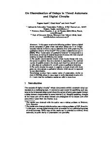
Example 2.2. Figure 2.1 shows a rooted transition system describing the behaviour of an automatic switch that controls a light as it can be found in a staircase or corridor in a hotel. Circles represent states. Their names are written beside them; in this case they are σ0 and σ1 . The initial state σ0 is indicated with a small incoming arrow. Arrows represent transitions. Their labels are given next to them; in this case they are on and off . The behaviour of the system can be described as follows. The state of the system in which the light is off is represented by σ0 , and σ1 represents the state in which the light is on on. People arrive at the staircase and turn on the switch (σ0 −−→ σ1 ). After a while the off
switch turns itself off (σ1 −−→ σ0 ). It could be the case that when the light is on, people press the switch anyway to reset the timer that controls the switching off. In such a case on the light stays on (σ1 −−→ σ1 ). We will use this simple switch as a running example. The intention is to show how it can be described in the different models we will discuss along this thesis. In this way we can compare the accuracy with which we can model the switch system, once we have added time and probability features. � When studying the behaviour of systems it is important to decide whether two systems described in terms of transition systems behave in the same manner. There are many reasons why it is important to equate systems. For instance, checking that a particular system completely satisfies its specification can amount to checking equivalence of the transition system modelling the system and the transition system describing the specification. Another reason is that whenever two systems show equivalent behaviour, one of them could be replaced by the other as part of a bigger system (up to some additional considerations). Many different ways to equate transitions systems have been defined, most of them during the last two decades. For a broad overview, the reader is referred to (van Glabbeek, 1990) and (van Glabbeek, 1993). In this thesis we will concentrate on several notions of bisimulation. A bisimulation (Milner, 1980; Park, 1981) can be seen as a game played by two players —each one of them following the rules given by a (rooted) transition system— in which one player proposes to perform a move —a transition— and the other is obliged to imitate it. At any moment of the game the role of proposing player and imitating player can be interchanged. Two players are bisimilar if none of them is capable to find a strategy to defeat his opponent. Definition 2.3. Let TS = (Σ, L, − → ) be a transition system. A relation R ⊆ Σ × Σ is
2.1. Transition Systems
15
off on σ0
σ1
σ1u
σ0u
on
σ0d
on
on
on
off
on σ1d
off
Figure 2.2: Two bisimilar transition systems
a bisimulation relation if R is symmetric and for all σ1 , σ2 ∈ R and for all � ∈ L the following transfer property holds: �
�
if σ1 −→ σ1� then σ2 −→ σ2� for some σ2� ∈ Σ such that σ1� , σ2� ∈ R. We say that two states σ1 and σ2 are bisimilar, notation σ1 ∼ σ2 , if there is a bisimulation R that relates them, i.e., σ1 , σ2 ∈ R. Two rooted transition systems (TS1 , σ1 ) and (TS2 , σ2 ) are bisimilar, if their initial states σ1 and σ2 are bisimilar in the (disjoint) union of TS1 and TS2 . � It is not difficult to prove that ∼ is the largest bisimulation relation and that it is an equivalence relation. The curious reader is referred to (Milner, 1989). Notation. Since we require that a bisimulation should be a symmetric relation, in many occasions we will give a relation and claim that its symmetric closure —i.e., the smallest symmetric relation that contains it— is a bisimulation. For such a reason, given a relation R over a certain domain, we use the notation Rs to refer to the symmetric closure of the relation R. Similarly we let R∗ denote the reflexive-transitive closure of R, that is, the smallest reflexive and transitive relation containing R. Finally, Req denotes the smallest equivalence relation containing R. We write Id for the identity relation. � Example 2.4. While in Example 2.2 the switch was intended to be a simple button, the transition system on the right of Figure 2.2 describes a switch with two positions: up and down. Thus, σ0u is the state in which the light is off and the switch is in upper position, σ1u represents the state in which the light is on and the switch is up, and σ0d and σ1d are the respective on and off states when the switch is down. It is not difficult to check that the relation R = { σ0 , σ0u , σ0 , σ0d , σ1 , σ1u , σ1 , σ1d }s is a bisimulation. Relation R is depicted with dotted lines in Figure 2.2.
�
16
Chapter 2. Preliminaries
As we have just done, to prove that two systems are bisimilar we have to exhibit a bisimulation. But usually this relation has information that we might find somehow redundant. So, we would like to give instead a smaller relation which omits that information. Hence, we define the notion of bisimulation up to ∼. Notice that it slightly differ from the traditional definition of Milner (1989). Definition 2.5. Let TS = (Σ, L, − → ) be a transition system. A relation R ⊆ Σ × Σ is a bisimulation up to ∼ if R is symmetric and for all σ1 , σ2 ∈ R and � ∈ L the following transfer property holds: �
�
if σ1 −→ σ1� then σ2 −→ σ2� for some σ2� ∈ Σ such that σ1� , σ2� ∈ (∼ ∪R)∗ .
�
In fact, finding a bisimulation up to ∼ suffices to show bisimilarity. This is stated by the following theorem. Theorem 2.6. Let R be a bisimulation up to ∼. Then R ⊆ (∼ ∪R)∗ ⊆∼. The proof of this theorem is analogous to and simpler than the proof of Theorem 3.6. In many cases, one would like to have completely automatic machinery to analyse the behaviour described by transition systems. To do so, algorithms for checking equivalences such as bisimulation have been devised (e.g. Paige and Tarjan, 1987; Kanellakis and Smolka, 1990; Fernandez, 1989), as well as algorithms to check if a transition system satisfies a given property expressed in a certain modal logic (e.g. Clarke et al., 1986; Godefroid and Wolper, 1991; Cleaveland, 1990; Wolper et al., 1983), and algorithms to derive complete test suites to test system implementations (e.g. Chow, 1978), among other kind of automatic analysis. All these algorithms do not operate over arbitrary transition systems. Since all of them require a complete search of the state space and transitions, an essential requirement is that transition systems are finite and hence termination of every algorithm is ensured. Other times, one may admit that a complete automatic analysis of the transition system is either impossible or too ambitious. In this case, a usual technique is simulation (e.g. Eertink, 1995). Simulation allows to study different possible executions of the systems and hence only the current state of the execution that is being traced is relevant. In such a case there is no need to require finiteness of the transition system. It is only important that from each state there is a finite number of outgoing transitions from which we can select one to execute. This kind of transition systems is called finitely branching1 . Definition 2.7. Let TS = (Σ, L, − → ) be a transition system. TS is finitely branching if for all σ ∈ Σ the set {σ −→ σ � | � ∈ L ∧ σ � ∈ Σ} �
is finite. We say that TS is finite if in addition it satisfies the property that the set of states Σ is finite. � 1
One may argue that for simulation purposes one still can have an infinite branching transition system if it is appropriately coded in a symbolic way. But in this case the obtained “symbolic” transition system needs to be finitely branching. In fact, in the rest of the thesis we discuss two classes of automata that abstractly model (uncountably!) infinitely branching transition systems.
2.2.
2.2
– A Common Language for Untimed Behaviours
17
– A Common Language for Untimed Behaviours
Process algebras were introduced at the end of the 70’s. The works of Tony Hoare (1978, 1985), on CSP, and Robin Milner (1980, 1989), on CCS, mark this point. During the 80’s, process algebras grew to end up as quite a mature method to model and analyse concurrent and communicating systems. Apart from CSP and CCS two other process algebras reached a distinct place in formal methods: ACP (Bergstra and Klop, 1985; Baeten and Weijland, 1990) and LOTOS (Brinksma, 1988; Bolognesi and Brinksma, 1989). In this section we discuss a process algebra for which we have selected the most relevant ingredients present in the algebras enumerated before. We call it clubs, standing for Common Language for Untimed Behaviours, and denote it by . The basic ingredient in process algebras is the action name. An action name —or simply, action— describes an activity that is performed by a system. This activity is assumed to be atomic, that is, it cannot be interrupted by any other activity when it is executed. Moreover, its execution does not consume any time. This concept is fundamental for the so-called interleaving models which are at the basis of this thesis. Assume a given process p that represents the behaviour of a system. An action a can be prefixed to p, thus becoming the process a; p, which first performs the action a and then shows the same behaviour as p. The most primitive process is the process 0 (read nil ) which does not show any behaviour; in other words, it does not do anything. In many cases a system offers the possibility to select one out of two possible behaviours p and q to be executed. This operation is called (non-deterministic) choice or sum and denoted by p + q. The previously described operations are called basic operations since all other operations can be eliminated in favour of these. The key operation for modelling concurrent systems, as it is the intention of process algebras, is the parallel composition or merge. p ||A q describes a process that executes p and q in parallel forcing the synchronisation of actions in the set A of action names. Either p or q can execute actions which are not in A independently. These actions interleave with the actions (not in A) of the other process. We will also consider two special notions of parallel composition. The left merge p || A q behaves exactly in the same way that p||A q does with the only exception that the first action (not in A) should be performed independently by process p. Similarly, the communication merge p |A q is a process that behaves like p ||A q with the restriction that the first action (in A) should be a synchronisation action. The left and communication merge are not really intended for the modelling of systems. Nevertheless they are essential to define a finite equational theory (Moller, 1990) as we will do in the next section. The last operation we consider is (action) renaming. Given a function f that takes an action name and changes it into another action name, process p[f ] behaves like process p but with the actions changed according to f . Apart from the just mentioned operations, we allow for recursive definitions. To do so, we consider process variables which are variables that can take processes as values. So, suppose p is a process that contains the process variable X. The recursive equation X = p defines the value of X as the one which solves that equation. In general, we choose the
18
Chapter 2. Preliminaries
unique solution to be the the minimal one following the approach of Milner (1989) instead of following the more general approach of Baeten and Weijland (1990) in which more than one possible solution is considered. Thus, equation X = a; X defines in X a process that performs infinitely many a’s, and Y = a; 0 + Y defines in Y the process that only performs one a. We can also define process variables by means of systems of recursive equations called recursive specifications, in which one process variable may be defined in terms of a process containing many other variables. Summarising, we define as follows. Definition 2.8. The language p
::=
is defined according to the following grammar
0 | a; p | p + p | p ||A p | p || A p | p |A p | p[f ] | X
where a is an action name belonging to the set A of action names, A ⊆ A is a synchronisation set, f : A → A is a renaming function, and X is a process variable belonging to the set V of process variables. A process variable is defined by an equation of the form X = p where p is a term. These kind of equations are called recursive equations. A recursive specification is a set E of recursive equations. Sometimes we will consider a distinguished process variable in the recursive specification E called root. � In general we will assume that prefixing and renaming have precedence over any other operator, and that + is the operation with lowest precedence. Thus, a; 0 + X[f ] ||A b; Y represents the term (a; 0) + ((X[f ]) ||A (b; Y )). Notice that we have not specified the precedence in some cases and hence some terms without parentheses, as for instance a; X[f ] or a; 0 ||A X || B b; Y , are ambiguous. We will always put parentheses to solve ambiguity in those cases. Example 2.9. In Example 2.2 we have described a switch in a stairway that can be switched on by people who arrive to the stair and it automatically switches off after a fixed period of time. So we have two processes in the system. The first is a simple process that describes the arrival of people: Arrival = on; Arrival The second is the switch itself: SwitchOff = on; SwitchOn SwitchOn = on; SwitchOn + off ; SwitchOff The complete system is described by the interaction of the switch and the people that arrive. Since people want to turn on the switch, both processes should synchronise on action on: System = Arrival ||on SwitchOff To simplify notation, we write ||a instead of ||{a} whenever the synchronisation set contains only one action. �
2.2.
– A Common Language for Untimed Behaviours
19
a
a
p −→ p�
a
a; p −→ p
p −→ p�
a
a
p + q −→ p�
a
q + p −→ p�
a
p −→ p�
a∈ /A
a
p ||A q −→ p� ||A q
p −→ p� a
q ||A p −→ q ||A p�
a
a
p −→ p�
a∈ /A
a
p ||A q −→ p� ||A q �
a
p −→ p� a
p || A q −→ p� ||A q
a∈ /A
p −→ p� a
a
p[f ] −−−→
a∈A
a
q −→ q �
p |A q −→ p� ||A q �
a∈A
a
p −→ p� f (a)
a
q −→ q �
p −→ p�
p� [f ]
a
X −→ p�
X =p
Table 2.1: Transition rules for
The behaviour of terms is given in terms of transition systems. The states of the transition system are terms. The transition relation is defined following Plotkin’s style (Plotkin, 1981). In the so-called structured operational semantics, the transitions that a process p can possibly perform are defined in terms of the transitions performed by the subprocesses out of which p is built. terms as it was previously described. Rules in Table 2.1 capture the behaviour of Process 0 does not have any outgoing transition meaning that it cannot do anything. a; p performs an action a and then behaves like p. p + q can perform any transition p or q can perform, and continues with the behaviour of the chosen process. p ||A q can independently perform any transition p or q can perform if this transition does not require synchronisation, i.e., if it is not labelled with an action in A. Synchronisation actions can be performed by p ||A q if both p and q can perform the same synchronisation action. p || A q can only perform transitions labelled with actions not in A whenever p can perform this transition. It continues by executing the “remaining” behaviour of p in parallel with q. p |A q can only perform transitions labelled with actions in A whenever p and q have an outgoing transition labelled with the same synchronisation action. Afterwards, the process behaves as a normal parallel composition. For each outgoing transition of p labelled with a, p[f ] has an outgoing transition renamed by f (a). Finally, a variable X, defined according to the equation X = p, has the same outgoing transitions as its defining process p. Formally, we have: Definition 2.10. The semantics of is defined according to the (labelled) transition → ) where and A are as in Definition 2.8 and − → is the least system TS( ) = ( , A, − relation satisfying the rules in Table 2.1. The semantics of a process p ∈ is defined by � the rooted transition system (TS( ), p).
20
Chapter 2. Preliminaries
Example 2.11. It is not difficult to check that the transition system defined by the process System in Example 2.9 is the one depicted in Figure 2.1 where state σ0 coincides with process Arrival ||on SwitchOff and σ1 with Arrival ||on SwitchOn. � In the previous section we mentioned that one of the reasons why we are interested in equating processes is that we would like to have the possibility of replacing a process by an equivalent one. Since the process will be replaced in a context, we need that such equivalence is a congruence. An equivalence relation is a congruence if for every pair of equivalent processes p and q, and any context C[ ], the processes C[p] and C[q] are also equivalent. The following theorem states that bisimilarity is a congruence for any context. Theorem 2.12. Let p and q two holds that C[p] ∼ C[q].
terms such that p ∼ q. For any
context C[ ], it
In many cases, congruence theorems can be proven using standard results in structured operational semantics by simply inspecting the shape of the rules (de Simone, 1984; Bloom et al., 1995; Groote and Vaandrager, 1992; Baeten and Verhoef, 1993; Fokkink and van Glabbeek, 1996, and many others). This is exactly the case with the previous theorem. We recall the path format of (Baeten and Verhoef, 1993). a Let Rel , Reli be transition relations (as they could be any transition relation −→ ), and let Pred , Predi be state predicates. Let op be an n-ary operation (for example, the binary operations + or ||A ). A rule is in path format if it has one of the following two forms, {pi Reli yi | i ∈ I} ∪ {Predj qj | j ∈ J} op(x1 , . . . , xn ) Rel p
(2.1)
{pi Reli yi | i ∈ I} ∪ {Predj qj | j ∈ J} Pred op(x1 , . . . , xn )
(2.2)
where vars = {x1 , . . . , xn } ∪ {yi | i ∈ I} is a set of distinct variables (over terms), and p, pi , qj are terms with free variables in vars2 . We say that a set of rules is in path format if all of its rules are. Based on (Groote and Vaandrager, 1992), Baeten and Verhoef (1993) proved that bisimilarity is a congruence for any operation whose semantics is defined with rules in path format, provided they satisfy the so-called well-foundedness condition. Later, Fokkink (1994b) dropped that condition thus proving the general case. It is not difficult to check that rules in Table 2.1 are in path format, and that consequently ∼ is a congruence for all operations, from which Theorem 2.12 follows. More recently, Rensink (1997) has proved a general congruence theorem for recursion with the only additional requirement that the rules should not have look-ahead, that is, the free variables of the pi ’s, qj ’s can only be those in {x1 , . . . , xn }. Thus, we can state the following theorem. 2
We have actually defined the so-called pure path format, which is sufficient for the purposes of this thesis. Moreover, we have omitted two formats of rules since they can always be equivalently defined in terms of those given here.
2.3. An Equational Theory for
21
˜ def Theorem 2.13. Let H = {Hi | i ∈ I} denote in general an indexed family over the index ˜ set I. Let p˜ and q˜ be two indexed families of processes with process variables only in X ˜ ˜ such that, for every family r˜ of processes and for every i ∈ I, pi [˜ r /X] ∼ qi [˜ r /X]. Define ˜ ˜ ˜ ˜ Yi = pi [Y /X] and Zi = qi [Z/X], i ∈ I. Then Yi ∼ Zi , for all i ∈ I. a
Consider the recursive equation X = a; 0 + X. Transition X −→ 0 can be deduced in infinitely many ways since a new, different proof tree can be constructed by choosing the right hand side of the + at different occasions. In this case, we say that variable X is defined with unguarded recursion. Unguarded recursion can also induce infinite branching in the obtained transition system as in the case of Y = a; 0 + (Y |a a; b; 0), in which the number of b’s that is performed depends on the number of times the right hand side of + a is chosen when proving Y −→ . Unguarded recursion is not always a desirable property. Especially if one thinks of the deduction system as something to be run on a computer. In the following, we formally characterise the notion of guarding. Definition 2.14. An occurrence of X is guarded in a term p ∈ if p has a subterm a; q such that this occurrence of X is in q. A term p is guarded if all the occurrences of its process variables are guarded. A recursive specification E is strictly guarded if the right-hand side of every recursive equation in it is a guarded term, i.e., for all X = p ∈ E, p is guarded. A recursive specification E is guarded if it can be rewritten into a strictly guarded recursive specification by unfolding the equations. (By “properly unfolding the equations” we mean that whenever X = p ∈ E and Y occurs unguarded in p, then we take the new specification E � = (E\{X = p}) ∪ {X = p[Y /q]} provided that Y = q ∈ E.) A recursive specification E is regular if it is guarded, it defines finitely many recursive equations (that is, E is a finite set), and for every recursive equation X = p ∈ E, the term p does not contain the operations ||A , || A , |A , and [f ]3 . � It is not difficult to prove that the semantics of a term whose variables are defined in a guarded recursive specification is a finitely branching transition system, and, conversely, that every finitely branching transition system can be written as a term with variables defined in a guarded recursive specification. Similarly, a term with variables defined in a regular recursive specification defines a finite transition system and vice-versa.
2.3
An Equational Theory for
In this section we introduce an equational theory for . An equational theory, also called abstract algebra or variety, is a structure containing a signature, which is a set of operations together with their arity, and a set of equations or axioms of the form t = t� , where t and t� are terms containing only operations in the signature and usually some free variables. We will use the terms axiomatic system or axiomatisation to refer to the set of axioms. 3
The notion of regular recursive specifications could be generalised to include all the operations by carefully avoiding recursion cycles within the so-called static operations. However, this definition is not that simple and it does not extend expressiveness. As a consequence, it is sufficient for us to restrict the definition.
22
Chapter 2. Preliminaries
A1 p + q = q + p
M
A2 (p + q) + r = p + (q + r) A3 p + p = p A4 p + 0 = p
p ||A q = p || A q + q || A p + p |A q
LM1 0 || A p = 0 LM2 a; p || A q = 0
if a ∈ A
LM3 a; p || A q = a; (p || A q)
if a ∈ /A
LM4 (p + q) || A r = p || A r + q || A r R1 0[f ] = 0 R2 (a; p)[f ] = f (a); (p[f ])
CM1 0 |A p = 0
R3 (p + q)[f ] = p[f ] + q[f ]
CM2 a; p |A a; q = a; (p ||A q)
if a ∈ A
CM3 a; p |A q = 0
if a ∈ /A
CM4 (p + q) |A r = p |A r + q |A r CM5 p |A q = q |A p Table 2.2: Axiom system for
The interest of giving an equational theory for and any other process algebra is twofold. First, the concept of algebra is fundamental in mathematics. That implies that the given axiom system will help for the understanding of the discussed process algebra and the concepts it involves. Second, the analysis and verification of systems described using the process algebra can be partially or completely carried out by mathematical proofs using the axiomatisation. Definition 2.15. The equational theory for is defined as follows. The signature contains the constant 0, the unary operators a; and [f ], for every a ∈ A and f : A → A, and the binary operations +, ||A , || A , and |A , for every A ⊆ A. The axiom system is given in Table 2.2. We identify with sig( ) and ax ( ) the signature and axiom system of . � An equational theory defines an abstract structure that talks in general about different possible models which we call algebras. An algebra is a structure (M, F, �) where M is a set of objects called carrier set, F is a set of functions over M, and � is a congruence relation on M for the functions in F 4 . We say that such an algebra models a given equational theory if for each operation in the signature there is a corresponding function in F with the same arity, and besides, The usual definition of algebra does not include the relation �. Instead, it considers equality to be the identity in M . Our definition is a simple generalisation but it does not define “more” algebras since it could be easily translated into the traditional definition by considering the quotient M/ � as carrier set, and the set of functions F/ � containing the functions of F with the usual transformation to range over M/ �. 4
2.3. An Equational Theory for
23
every law t = t� proved using the axiom system (together with equational reasoning) holds when the = symbol is replaced by the � relation, every operation in the terms t and t� is replaced by their respective function in the algebra, and the free variables are consistently replaced by any object in M. In this case, we usually say that the equational theory is sound for the algebra. Conversely, we say that an equational theory is complete for the algebra if for any two objects in M that are equivalent according to �, they can be proved to be equivalent by using the axiom system. In the following we state soundness and completeness of with bisimilarity being the equivalence relation. We ambiguously use the same symbol to represent an operation in the signature and its respective function in the algebra. Theorem 2.16 (Soundness). The equational theory of sound for the algebra ( , sig( ), ∼)
given in Definition 2.15 is
The style of proving this theorem is classic in process algebra (e.g. Milner, 1989; Baeten and Weijland, 1990; Baeten and Verhoef, 1995, see also Aceto et al. 1994 where a systematic approach is reported). Because of the characteristics of equational reasoning, it is enough to consider only the axioms instead of any possible law derived from them as the definition of soundness requires. We do that as follows: for each axiom t = t� in ax ( ) define a bisimulation relation R containing every possible pair p, p� where p and p� are respective instances of t and t� with a consistent substitution of the free variables. As an example, the relation { p + p, p | p ∈ } ∪ { p, p | p ∈ }, which can be proved to be a bisimulation, states soundness for axiom A4. When we introduced we mentioned that operations 0, a; , and + are basic operations since the other operators can be eliminated in favour of them. That is, every term has a containing only provable equivalent basic term. In fact this is valid for the subset of c closed terms, i.e., terms not containing process variables. We denote by the set of closed terms. Besides, we denote by b the set of basic terms, i.e., the subset of c containing only those terms formed using the operations 0, a; , and +. To state elimination we transform some axioms and derived theorems into a strongly terminating rewriting system (Klop, 1992) and show that the normal form (i.e., the term that cannot be reduced any further) is a basic term. This is a usual technique in process algebras (see e.g. Bergstra and Klop, 1985; Baeten and Weijland, 1990; Baeten and Verhoef, 1995). In fact, for our case we consider axioms R1–R3, M, LM1–LM4, and CM1–CM4 as rewrite rules with direction left to right. For instance, from M we take the rewrite rule p ||A q → p || A q + q || A p + p |A q Since including CM5 as a rewrite rule would not give a strongly terminating rewrite system (i.e., a system in which there is no infinite reduction sequence), we do not do so, but use it to derive three more rules which give us the desired rewriting system. These rules are actually an appropriate variation of CM1, CM3, and CM4 in which the terms are commuted respect to the communication merge. For instance, using axioms CM4, CM5, and A4 we can prove that p |A (q + r) = p |A q + p |A r
24
Chapter 2. Preliminaries
and transform it also in a rewrite rule. Theorem 2.17 (Elimination). For every closed term p ∈ c there exists a basic term q ∈ b such that p = q can be proven using the axiom system ax ( ). Elimination explains which are the fundamental concepts in the theory —namely, the basic operations— by stating which are the minimal elements we can construct, and still keep the full expressive power of the theory. But elimination does have another important role. It is a key tool in proving completeness. Because of elimination we can restrict to prove completeness of the sub-theory induced by b and then have completeness of c for free. To be more precise, take two terms p and q in c such that p ∼ q. Because of elimination there are p� , q � ∈ b such that p = p� and q = q � are provable in ax( ), and by soundness and transitivity of ∼, p� ∼ q � . So proving that p� = q � is provable in ax( ), we have that p = q is also provable in ax( ). The proof that the sub-theory containing the basic operations in the signature and axioms A1–A4 as axiom system is complete for bisimulation in b is given in (Milner, 1989). Theorem 2.18 (Completeness). The equational theory of complete for the algebra ( c , sig( ), ∼).
given in Definition 2.15 is
Notice that completeness only holds for the set of closed terms. When process variables and recursion are introduced, additional laws are needed (Milner, 1984, 1989). As simple counterexample we mention that the processes a; 0 and Y , defined by Y = a; 0 + Y , are bisimilar, but they cannot be proven equivalent in ax( ). The elimination theorem tells us which are the basic operations. A more elaborated theorem, the so-called expansion law , complements elimination by saying how the nonbasic operations like the parallel composition can be decomposed in terms of the basic ones. � � � Theorem 2.19 (Expansion law). Let p = ai ; pi and q = bj ; qj where k∈K rk denotes the process r1 + r2 + · · · + rn , if K = {1 . . . n}, or 0, if K = ∅. Then, the following equalities can be proven from the axiom system ax ( ). � � � ai ; (pi ||A q) + bj ; (p ||A qj ) + ai ; (pi ||A qj ) p ||A q = ai ∈A /
p[f ] =
�
bj ∈A /
ai =bj ∈A
f (ai ); (pi[f ])
The last property we discuss in this introductory chapter is conservative extension. When developing a complex equational theory on top of a more basic one it is interesting to know whether the properties of the (original) basic theory are preserved in the extended one. More precisely, we can say that, given two equational theories E1 and E2 such that the signature of E1 is contained in the one of E2 , E2 is a conservative extension of E1 if exactly the same theorems regarding only the original terms, i.e., those from E1 , can be proven in the axiom systems of both E1 and E2 ,. Formally, we say that E2 is a conservative
2.3. An Equational Theory for
25
extension of E1 , if sig(E1 ) ⊆ sig(E2 ), and for every pair of closed terms p and q whose operations are in sig(E1 ), p = q is provable in ax (E1 ) if and only if it is also provable in ax (E2 ). As an example we can state the following theorem in the context of . Theorem 2.20 (Conservative extension). The equational theory of given in Definition 2.15 is a conservative extension of the basic equational theory whose signature are the basic operations and its axiom system contains only the axioms A1–A4. The technique for proving this theorem has been formalised in (Verhoef, 1994) and generalised in (D’Argenio and Verhoef, 1997). From the latter, we recall that conservative extension can be guaranteed if the following conditions hold: 1. Every axiom of ax (E1 ) is provable in ax (E2 )5 , 2. E1 is sound and complete for (M1 , F1 , �1 ) and E2 is sound for (M2 , F2 , �2 ), and 3. (M2 , F2 , �2 ) is a model conservative extension of (M1 , F1 , �1 ), that is, M1 ⊆ M2 , F1 ⊆ F2 , and for all t, t� ∈ M1 , t �1 t� ⇐⇒ t �2 t� . In the context of structured operational semantics, model conservative extension reduces, in many occasions, to check two simple conditions. The first one can be carried out by simple inspection of the set of rules that defines the semantics of the terms (in our case the rules in Table 2.1). The new rules, that is, the rules introduced in the extended process algebra, should not introduce new relations or predicates for the terms in the old signature. Formally, take SOS 1 and SOS 2 to be the set of rules defining the semantics of the terms in sig(E1 ) and sig(E2 ) respectively. Then it should be the case that SOS 1 ⊆ SOS 2 and for every new rule in (SOS 2 −SOS 1 ) —which has the shape of rule (2.1) or (2.2), see page 20— the operation op should not belong to the old signature sig(E1 )6 . The second condition requires that the equivalence relation which is being axiomatised is defined in terms of predicates and relations only, as it is the case of bisimulation. Under these conditions conservative extension follows. So, for Theorem 2.20, the original set of rules are those for a; and + in Table 2.1 (i.e., the three first rules), all the others are the “new rules”. Clearly, the new rules only define the semantics of the new operations ||A , || A , |A , and [f ]. From the previous discussion, the theorem is hence proved.
Actually (D’Argenio and Verhoef, 1997) asks that ax (E1 ) ⊆ ax (E2 ), but this condition can be straightforwardly relaxed to what we ask here. 6 This condition is stronger than that in (D’Argenio and Verhoef, 1997), which, however, is much more technically involved. For our purposes, the stronger condition will suffice. 5
Part Two Timed Systems
‘Er, how are we for time?’ he said ‘have I just got a min—’ And so the Universe ended. Douglas Adams, The Restaurant at the End of the Universe. London, 1980
Chapter 3 Timed Transition Systems Timed transition systems are a variant of transition systems which incorporate information about time. The usual way is to consider non-negative real numbers as part of the label on the transition relation. These numbers are intended to represent the necessary amount of time to move from the source state to the target state. There have been several definitions of timed transition systems. The most widely used contains transitions labelled with an action name or with a time label (a non-negative real number). Thus this kind of timed transition system is nothing else but a transition system with A ∪ IR≥0 as set of labels. Usually some consistency requirements are imposed on the timed transitions —such as time additivity and time determinism (see Yi, 1990)— to ensure that time progresses as expected. Another approach is to consider instead transitions labelled with both action names a(d)
and time. Thus, σ −−−→ σ � means that, at a state σ, it is possible to execute action a after idling for d time units and move to the new state σ � . This approach has been used in real-time ACP (Baeten and Bergstra, 1991; Klusener, 1993), to name the most popular case, and is the one that we use as a concrete model to describe real time behaviours. In this chapter, we define timed transition systems and give the notion of equivalence we use to equate timed behaviour. This equivalence is a simple variation of bisimulation that takes the passage of time into account. The model we present is based on the model defined by Klusener (1993), although its formalisation is inspired by (Yi, 1990).
3.1
The Model
Timed transition systems are a variant of transition systems which incorporate information about time. Time is added by including a class of labels taken from a time domain. A time domain is a totally ordered monoid with an addition operation + and a neutral element 0 that is also the minimum in the ordering, such that d ≤ d + d� for all d and d� belonging to the time domain, and d + d� ≤ d if and only if d� = 0. We choose the set IR≥0 of non-negative real numbers as our time domain.
29
30
Chapter 3. Timed Transition Systems
→ , U) Definition 3.1. A timed transition system is a structure TTS = (Σ, A × IR≥0 , − where • Σ is a set of states; • A is a set of actions; • − → ⊆ Σ × (A × IR≥0 ) × Σ is the transition relation; and • U ⊆ IR≥0 × Σ is the until predicate. We write a(d) instead of (a, d) and, as for transition systems (see Definition 2.1), we use the a(d)
a(d)
a(d)
shorthand notations σ −−−→ σ � , σ −−−→ , and σ −−−→ / . We also write Ud (σ) if d, σ ∈ U. In addition, for all σ ∈ Σ and a ∈ A, TTS should satisfies the following axioms: Until
∀d, d� ∈ IR≥0 . Ud (σ) ∧ d� < d =⇒ Ud� (σ);
Delay
∀d ∈ IR≥0 . σ −−−→ =⇒ Ud (σ).
a(d)
As for transition systems, it will be convenient to distinguish an initial state σ0 ∈ Σ. In this case we call the structure (TTS, σ0 ), a rooted timed transition system. � a(d)
The intended meaning of a transition σ −−−→ σ � is that, whenever the system is in state σ, it can change to state σ � by performing an action a after idling d units of time. Intuitively, Ud (σ) means that the system can idle in a state σ at least d units of times. Axiom Until states that if the system can idle d units of time in a state σ, then it is also able to idle there for less time. Axiom Delay says that every time that the system is in a state σ in which an action a can be performed after idling d units of time, it should be explicitly said that the system in state σ can idle until that time. The reader might think that predicate U is redundant, however this is not the case. Predicate U is crucial to model features like urgency, time divergence and time deadlock. We briefly explain each of them. • A system in state σ is urged to perform an action a at time d if it cannot idle any further in that state, and it has the possibility to do this action. Formally we can say a(d)
that state σ is urgent at time d if σ −−−→ for some action a and there is no d� > d such that Ud� (σ). • A system is time divergent in state σ if it can idle there for ever, that is, if Ud (σ) a(d)
for all d ∈ IR≥0 . Notice that, in this case, if σ −−−→ , for a particular d, the system may still choose not to do action a and keep idling. Compare this with the case of urgency in which the action becomes a mandatory escape as time progresses. • Finally, a system has a time deadlock in a state σ if it can idle there until a time d at which it is not allowed to idle anymore but at the same time there is no possible a(d)
/ for any a ∈ A, and there is no d� > d action outgoing from σ, i.e., Ud (σ), σ −−−→ such that Ud (σ).
3.2. Timed Bisimulation
31
The features we have just discussed are quite important to model and analyse systems. In fact, they are crucial for the verification of so-called hard real-time systems. For instance, urgency is the key component to describe time-outs, and a time deadlock may represent an endpoint in the lifetime of the described system, usually with catastrophic consequences. Example 3.2. In this example we consider the same switch in a stairway that we already described in Example 2.2, but we explicitly model an additional feature. We fix the time when the light must be turned off. So, assuming that the light is turned off 2 minutes after the last time the on button was pressed, the switch can be modelled by the timed transition system (Σ, A × IR≥0 , − → , U) where Σ = {σ0 , σ1 }
A = {on, off }
on(d)
Ud (σ0 ) ⇐⇒ 0 ≤ d
on(d)
Ud (σ1 ) ⇐⇒ 0 ≤ d ≤ 2
σ0 −−−−→ σ1 ⇐⇒ 0 ≤ d σ1 −−−−→ σ1 ⇐⇒ 0 ≤ d ≤ 2 off (2)
σ1 −−−−→ σ0 Notice that in state σ0 the system is allowed to idle indefinitely, while in state σ1 , when the light is on, the system cannot idle beyond 2 minutes. After idling 2 minutes the system is forced to execute either the action off or on. Notice that action off can only take place after idling exactly 2 minutes and not before. While in σ0 the time diverges, in σ1 an urgency situation arises at time 2, and actually, it urges for a decision between turning off the light or resetting the timer by pressing on again. If we choose σ0 to be the initial state, we can model the switch as a rooted timed transition system. � The kind of timed transition system we have defined is particular to this thesis. However their relation with existing models is straightforward. To begin with, our model is based on (Klusener, 1993). The main difference is that Klusener uses absolute time, that is, the a(d)
time stamp (i.e. the d in −−−→ and Ud ) indicates the time elapsed since the very beginning of the process, while we use relative time, meaning that the time stamp refers to the time elapsed since the current state has been reached (or, alternatively, since the last action occurred). In fact, predicate U is borrowed from (Klusener, 1993). Here, we formalised its behaviour in a relative time setting by adding the axioms Until and Delay. But probably the most widely used timed transition system model is the one that considers discrete actions (i.e. actions in A) and timed actions separately as labels of the transition relation (see Yi, 1990, 1991, for a formalisation). Under the usually accepted conditions of time determinism and time additivity property (Yi, 1990), this model is equivalent to ours.
3.2
Timed Bisimulation
To equate timed transition systems we use a variant of bisimulation semantics (see Definition 2.3), which is called timed bisimulation.
32
Chapter 3. Timed Transition Systems
→ , U) be a timed transition system. A relation R ⊆ Definition 3.3. Let (Σ, A × IR≥0 , − Σ × Σ is a timed bisimulation relation if R is symmetric and for all σ1 , σ2 ∈ R and for all a ∈ A and d ∈ IR≥0 , the following transfer properties hold: a(d)
a(d)
1. if σ1 −−−→ σ1� then σ2 −−−→ σ2� for some σ2� ∈ Σ such that σ1� , σ2� ∈ R; and 2. if Ud (σ1 ) then Ud (σ2 ). We say that two states σ1 and σ2 are timed bisimilar, notation σ1 ∼t σ2 , if there is a timed bisimulation R that relates them, i.e., σ1 , σ2 ∈ R. Two rooted timed transition systems (TTS1 , σ1 ) and (TTS2 , σ2 ) are timed bisimilar, if their initial states σ1 and σ2 are timed bisimilar in the (disjoint) union of TTS1 and TTS2 . � Notice that by symmetry of R, the second transfer property could be also written as “Ud (σ1 ) if and only if Ud (σ2 )”. Relation ∼t can be proved to be a timed bisimulation and an equivalence relation following the same proof as for ∼. Notice that by definition ∼t contains all timed bisimulations, which makes it the largest one. As in Section 2.1, we refer to (Milner, 1989) for the proof that shows ∼ is an equivalence and the largest bisimulation. Thus, we state the following theorem. Theorem 3.4. 1. ∼t is a timed bisimulation relation, and 2. ∼t is an equivalence relation over the set of states Σ. As for bisimulation, we can define the notion of timed bisimulation up to ∼t , and it is also the case that finding a timed bisimulation up to ∼t suffices to show timed bisimilarity. Definition 3.5. Let (Σ, A × IR≥0 , − → , U) be a timed transition system. A relation R ⊆ Σ × Σ is a timed bisimulation relation up to ∼t if R is symmetric and for all σ1 , σ2 ∈ R and for all a ∈ A and d ∈ IR≥0 , the following transfer properties hold: a(d)
a(d)
1. if σ1 −−−→ σ1� then σ2 −−−→ σ2� for some σ2� ∈ Σ such that σ1� , σ2� ∈ (∼t ∪R)∗ ; and 2. if Ud (σ1 ) then Ud (σ2 ).
�
Theorem 3.6. Let R be a timed bisimulation up to ∼t . Then R ⊆ (∼t ∪R)∗ ⊆∼t . Proof. It is sufficient to prove that (∼t ∪R)∗ is a timed bisimulation. It is not difficult to check that (∼t ∪R)∗ is � symmetric. So, it remains to check that the transfer properties hold. Since (∼t ∪R)∗ = n≥0 (∼t ∪R)n we prove that by induction on n. � The case for n = 0 is trivial. So, suppose σ1 , σ2 ∈ 0≤h≤n+1 (∼t ∪R)h . Then, there is � a σ ∈ Σ such that σ1 , σ ∈ 0≤h≤n (∼t ∪R)h and σ, σ2 ∈∼t ∪R.
3.2. Timed Bisimulation
33 a(d)
a(d)
1. Suppose σ1 −−−→ σ1� . Then, σ −−−→ σ � and σ1� , σ � ∈ (∼t ∪R)∗ , for some σ � ∈ Σ, by a(d)
a(d)
induction hypothesis. Besides, σ −−−→ σ � implies σ2 −−−→ σ2� and either σ � , σ2� ∈∼t or σ � , σ2� ∈ (∼t ∪R)∗ , for some σ2� ∈ Σ, depending on whether σ, σ2 ∈∼t or a(d)
σ, σ2 ∈ R. Thus, σ2 −−−→ σ2� and σ1� , σ2� ∈ (∼t ∪R)∗ . 2. Clearly Ud (σ1 ) implies Ud (σ) and Ud (σ) implies Ud (σ2 ), from which this transfer property follows. Q.E.D.
Chapter 4 Timed Automata Although timed transition systems give an adequate mathematic framework to represent the behaviour of real-time systems, they certainly are inappropriate to do automatic analysis due to their intrinsically infinite size, let alone to use it as a formalism for the specification of timed systems. Therefore, there is a need to represent a timed system in a symbolic way. Probably, the most successful formalism to symbolically specify real-time systems is the timed automata model (Alur and Dill, 1990, 1994; Henzinger et al., 1994). A timed automata is a transition system annotated with timers. The timers, which are called clocks, can be reset to 0 and they increase according time passes. Constraints on the value of the clocks will determine whether a transition may or must be executed. Timed automata have been successfully used in automatic verification of real-time systems, particularly by model checking properties given in an appropriate temporal logic (Alur et al., 1993; Henzinger et al., 1994). Many tools has been implemented using this methodology. In particular, the tools Kronos (Yovine, 1993; Olivero, 1994; Bozga et al., 1998) and Uppaal (Larsen et al., 1997; Pettersson, 1999) reached an appropriate level of maturity; they have been satisfactorily used in many actual case studies (see, e.g., Bengtsson et al., 1996a; Maler and Yovine, 1996; D’Argenio et al., 1997b). In this chapter we introduce the timed automata model (actually, a slight variant of the traditional model introduced by Henzinger et al., 1994), and define its semantics in terms of timed transition systems. We also define some equivalence relations directly on timed automata following the bisimulation style. These notions take into account the symbolic information and, since they are strictly finer than timed bisimulation, they are particularly useful to prove equivalence of behaviour in many cases, without the need to go down to the concrete behaviour given by timed transition systems.
4.1
Clocks and Clock Constraints
In Example 3.2, we described a set of possible transitions by simply saying on(d)
σ1 −−−−→ σ1 ⇐⇒ 0 ≤ d ≤ 2 35
36
Chapter 4. Timed Automata
v(x) ≤ d |= v(x ≤ d)
v(x) − v(y) ≤ d |= v(x − y ≤ d)
|= v(φ) |= v(φ� ) |= v(φ ∧ φ� )
d ≤ v(x) |= v(d ≤ x)
d ≤ v(x) − v(y) |= v(d ≤ x − y)
|� = v(φ) |= v(¬φ)
Table 4.1: Satisfaction of a clock constraint in a valuation v
To do this, the constraint 0 ≤ d ≤ 2 is crucial, and similarly for the definition of Ud . In fact, constraints like this are the ones we are going to use to describe symbolically the timed behaviour of systems. Apart from that, we are going to consider an additional ingredient: the so called clock variables or clocks for short. A clock is a variable that allows us to record the passage of time. Like a chronometer, they can be reset to 0 and inspected at any moment to see how much time has passed since their resets. By having several different clock variables we can measure and compare the timing of different events, as we define all clocks to increase at the same rate. The way to inspect clocks is by means of constraints defined as follows. Definition 4.1. Given a set of clock variables C we define the set Φ of clock constraints according to the following grammar φ
::=
x ≤ d | d ≤ x | x − y ≤ d | d ≤ x − y | (φ ∧ φ) | (¬φ)
where d ∈ IR≥0 and x, y ∈ C. If φ is a clock constraint in Φ, we denote with var(φ) the set of clock variables occurring in φ. � We notice that abbreviations like tt, ff , x = d, x > d, x − y < d, φ ∨ φ� , x ∈ [d, d� ), can def def be defined in Φ. For instance, tt ⇐⇒ x − x ≤ 0 or x ∈ [d, d�) ⇐⇒ (d ≤ x) ∧ ¬(d� ≤ x). Constant numbers in clock constraints are usually restricted to non-negative integers. This is required for decidability matters when doing analysis of real time systems. Since in our work, we are not bound to decidability concerns, we will not impose this restriction. Nonetheless, this restriction must be considered as soon as any analysis technique is applied in any framework we are going to discuss afterwards. The satisfaction of a constraint depends on the value each clock takes. Hence, the satisfaction of a constraint is subject to a valuation. A valuation is a function v : C → IR≥0 that assigns a non-negative real value to each clock. We let V denote the set of all valuations. We define the satisfaction of a constraint φ in a valuation v, denoted by |= v(φ), inductively in the usual way (see Table 4.1). We say that a constraint φ holds, and denote |= φ, if φ is satisfied in every valuation v, that is for all v, |= v(φ).
4.2. The Model
37
Since a valuation is a snapshot of the clock values in a particular instance, we need operations that manipulate valuations consistently as time evolves. The first operation defines the valuation that is obtained after d units of time has passed since we observed an old valuation v. This valuation is denoted by v + d and defined by def
(v + d)(x) = v(x) + d for all clock x ∈ C. The second operation gives the new valuation after resetting a set of clocks C in a given valuation v. We denote it by v[C 0], C ⊆ C, and define, for all x∈C � 0 if x ∈ C def v[C 0](x) = . v(x) if x ∈ /C �→
�→
Recall that axiom Until in Definition 3.1 states that if the system can idle d units of time at a given sate, then it is also able to idle there for less time. We can also characterise the class of clocks constraints that meet a similar property. They are called past-closed constraints. A clock constraint φ ∈ Φ is past-closed if for every valuation v ∈ V and time d ∈ IR≥0 , |= (v + d)(φ) =⇒ |= v(φ) We let Φ denote the set of all past-closed constraints.
4.2
The Model
In Example 3.2, we described a simple system using timed transition systems. Since the number of transitions was uncountably large, we resorted to some symbolic description. Although not in our example, the number of states may also be uncountable and we would need to mention all of them also in a symbolic way. Timed automata were introduced precisely to represent timed behaviour in such a symbolic manner. A timed automaton is basically a transition system whose arrows and nodes are decorated with clocks and clock constraints. Definition 4.2. A timed automaton is a structure TA = (S, A, C, ✲, ι, κ) where: • S is a set of locations; • A is a set of actions; • C is a set of clocks; • ✲⊆ S × (A × Φ) × S is the set of edges; • ι : S → Φ is the invariant assignment function; and
38
Chapter 4. Timed Automata
s0
on
s1 x x≤2
on
x = 2, off Figure 4.1: A timed automaton representing a switch in a stairway • κ : S → ℘(C) is the clock resetting function. ✲ s� instead of (s, a, φ, s� ) ∈ ✲ and s ✲ whenever there is an s� such We write s a,φ✲ � that s s. In many occasions it will be of convenience to distinguish an initial location s0 ∈ S. In this case we call the structure (TA, s0 ), a rooted timed automaton. � a,φ
a,φ
✲ s� intuitively means that when the system is in location s it could change to s location s� by performing an action a only in those moments in which the clock constraint φ, called guard , is satisfied. Immediately afterwards, all clocks in κ(s� ) are reset. A timed automaton is allowed to idle in a location s only as long as the associated invariant ι(s) is satisfied. a,φ
Example 4.3. The switch of Example 3.2 can be described by the timed automaton def System = (S, A, C, ✲, ι, κ) where S = {s0 , s1 } A = {on, off } C = {x}
s0 s1 s1
on,tt✲
s1 s1 off ,x=2✲ s1 on,tt✲
κ(s0 ) = ∅ κ(s1 ) = {x}
ι(s0 ) = tt ι(s1 ) = (x ≤ 2)
We assume s0 to be the initial location. The timed automaton is depicted in Figure 4.1. There, we represent the locations by circles which are divided in two halves. Inside the upper half we enumerate the clocks to be reset according to κ. In the lower half, we write the invariant of the location assigned according to ι. Edges are represented by arrows labelled with the corresponding action and clock constraint. To avoid messing the picture we do not write the constraint tt, the empty set, and the braces enclosing sets. � Timed automata were introduced by Alur and Dill (1990, 1994) although the concept of invariant was added later in the so called timed safety automata (Henzinger et al., 1994; Nicollin et al., 1992, 1993). The model we have defined is a slight variation of the timed safety automata model. We defined the clock resettings to be associated to locations instead of edges. The main reason to do so is that it allows a simpler treatment when using timed automata as the underlying semantic model of a real-time process algebra (see Chapter 5). Our approach allows to have a prefixing operation (like in ) and a separate operation
4.3. Semantics for Timed Automata
39
representing the clock resetting and yet having a straightforward semantics. Compare with the process algebra of (Yi et al., 1994; Pettersson, 1999) in which the prefix operation is integrated with both the clock resetting and the guard. Nonetheless, this variation does neither restrict nor add expressiveness. Our timed automata can be translated into timed safety automata by “pulling” the clock resettings a,φ✲ � out of the target location into the arrow, that is, an edge s s will be translated � a,φ,κ(s )✲ � into s s . Conversely, a timed automaton with resettings on the edges could be transformed by “pushing” the clock resetting into the target state, i.e., given an edge def a,φ,C✲ � a,φ✲ � s s we define s s and κ(s� ) = C. In case many edges with different clock resettings go to the same location, this state is “split” into different locations, one for each different set of clocks. Remark 4.4. We remark that transition systems are a subset of timed automata. In fact, every transition system can be translated into a timed automaton in the following way. Given the transition system (Σ, A, − → ), we define the timed automaton (Σ, A, ∅, ✲, ι, κ) a a,tt✲ � σ whenever σ −→ σ � . That is, where κ(σ) = ∅ and ι(σ) = tt for all σ ∈ Σ, and σ a transition system is a timed automaton in which the occurrence of activity is not bound to any time. Conversely, every timed automaton which is not bound to time can be straightforwardly translated into a transition system by removing all the “additional ingredients”. Timed automata whose activity are time dependent cannot be translated into transition systems without losing information. � In the same way we did for transition systems in Definition 2.7, we can characterise whether a timed automaton is finite or finitely branching. The way in which we define it is quite the same. Definition 4.5. Let TA = (S, A, C, ✲, ι, κ) be a timed automaton. TA is finitely branching if for all s ∈ S the set {s
a,φ✲
s� | a ∈ A ∧ φ ∈ Φ ∧ s� ∈ S}
is finite. We say that TA is finite if the set of locations S is also finite.
�
It has been shown in (Alur et al., 1993; Alur and Dill, 1994) that reachability analysis is possible for finite timed automata, provided that the constants used in the clocks constraints are integers, or can be scaled to integers.
4.3
Semantics for Timed Automata
In Chapter 3 we introduced a concrete model to describe timed behaviour: the timed transition systems. In the previous section we defined timed automata to symbolically specify timed systems, but we only explained intuitively their behaviour. In the following we define the semantics of timed automata in terms of timed transition systems.
40
Chapter 4. Timed Automata
Definition 4.6. Let TA = (S, A, C, ✲, ι, κ) be a timed automaton. The interpretation → , U) where of TA is given by the timed transition system TTS(TA) = (S × V, A × IR≥0 , − − → and U are defined as the least sets satisfying the following rules: 0] + d)(ι(s)) |= (v[κ(s) Ud (s, v) �→
a,φ✲
s�
|= (v[κ(s) a(d)
(s, v) −−−→ (s� , (v[κ(s)
0] + d)(φ ∧ ι(s)) �→
Act
s
�→
Idle
0] + d))
The interpretation of the rooted timed automaton (TA, s0 ) in the initial valuation v0 ∈ V is given by the rooted timed transition system (TTS(TA), (s0 , v0 )). � Since ι(s) is a past-closed constraint, it follows that TTS(TA) satisfies axiom Until in a(d)
0] + d)(ι(s)) and Definition 3.1. Moreover, notice that if (s, v) −−−→ then |= (v[κ(s) so Ud (s, v), which implies that axiom Delay holds as well. Hence, TTS(TA) is indeed a timed transition system. Rule Idle states that the system is allowed to idle in a location s which was reached with clocks valuated according to v, if after resetting the clocks in κ(s) and letting d units of time pass, the invariant ι(s) still holds. Rule Act explains the case in which a transition a,φ✲ � s was reached when the can take place. So, if a location s with an outgoing edge s clocks where valued according to v, action a can be executed after d units of time if, in addition to the invariant ι(s), the guard φ holds in valuation v after resetting the clocks in κ(s) and idling for d units of time. Once the action is executed, the system changes its location to s� and hence it is reached with the clocks valued according to the valuation in 0] + d. which s was left, that is, v[κ(s) �→
�→
Example 4.7. By Definition 4.6, the semantics of the timed automaton in Example 4.3 → , U) where is the timed transition system TTS(System) = (S × V, A × IR≥0 , − on(d)
(s0 , (x := d� )) −−−−→ (s1 , (x := d� + d)) ⇐⇒ d, d� ∈ IR≥0 on(d)
(s1 , (x := d� )) −−−−→ (s1 , (x := d)) ⇐⇒ 0 ≤ d ≤ 2, d� ∈ IR≥0 off (2)
(s1 , (x := d)) −−−−→ (s0 , (x := 2)) ⇐⇒ d ∈ IR≥0 Ud (s0 , (x := d� )) ⇐⇒ d, d� ∈ IR≥0 Ud (s1 , (x := d� )) ⇐⇒ 0 ≤ d ≤ 2, d� ∈ IR≥0 Choosing valuation x := 0 to be initial, we see that (TTS(System), (s0 , (x := 0))) is a possible interpretation for the rooted timed automaton. �
4.4. Equivalences on Timed Automata
4.4
41
Equivalences on Timed Automata
In the following we define several notions of equivalences for timed automata. In the first place, we extend timed bisimilarity to timed automata. This is rather straightforward since we do that on top of the semantics of timed automata in terms of timed transition systems. Definition 4.8. Two locations s1 and s2 of a timed automaton TA are timed bisimilar , notation s1 ∼t s2 , if they are timed bisimilar in TTS(TA) for all valuations, that is, if for every v ∈ V, (s1 , v) ∼t (s2 , v). Two rooted timed automata (TA1 , s1 ) and (TA2 , s2 ) are timed bisimilar if their interpretations are timed bisimilar for every initial valuation, that is, if (TTS(TA1 ), (s1 , v0 )) and (TTS(TA2 ), (s2, v0 )) are timed bisimilar for every valuation v0 ∈ V. � Since ∼t is an equivalence relation on the set of the actual states, it is immediate that ∼t is also an equivalence relation on the set of locations S. Timed bisimulation is our preferred equivalence since it precisely captures the timed and branching behaviour of a timed system. However, proving things to be timed bisimilar directly on the timed transition system can be quite difficult. In many cases, we do not need to resort to the definition of timed bisimulation to prove that two timed automata are timed bisimilar. We can state that without leaving the symbolic description by using stronger equivalences defined at this level. In the following, we define three different notions of equivalences and we relate them to each other and to timed bisimulation. We show that timed bisimulation is the weakest relation and isomorphism is the strongest one. To start with, we define the notion of isomorphism on timed automata. Definition 4.9. Let TA = (S, A, C, ✲, ι, κ) and TA� = (S � , A, C, ✲ � , ι� , κ� ) be two timed automata. We say that TA and TA� are isomorphic, notation TA ∼ = TA� , if there is a bijective function I : S → S � such that 1. s
a,φ✲
s� ⇐⇒ I(s)
a,φ✲ �
I(s� ),
2. ι(s) = ι� (I(s)), and 3. κ(s) = κ� (I(s)). In this case we say that the function I is an isomorphism. Two rooted timed automata � (TA, s0 ) and (TA� , s�0 ) are isomorphic if in addition I(s0 ) = s�0 . The definition of isomorphism could be extended by allowing a bijection on the clocks and another on the actions. For our purposes, the simpler Definition 4.9 is sufficient. Although isomorphism is a simple notion, it is certainly too strong. In the following we define a structural bisimulation which, although strong, it will be useful in many cases since it is defined in the style of bisimulation but directly on timed automata.
42
Chapter 4. Timed Automata
Definition 4.10. Let (S, A, C, ✲, ι, κ) be a timed automaton. A relation R ⊆ S × S is a structural bisimulation if R is symmetric and for all a ∈ A and φ ∈ Φ, whenever s1 , s2 ∈ R the following transfer properties hold: 1. if s1
a,φ✲
s�1 , then there is a s�2 ∈ S such that s2
a,φ✲
s�2 and s�1 , s�2 ∈ R;
2. ι(s1 ) = ι(s2 ); and 3. κ(s1 ) = κ(s2 ). We say that two locations s1 and s2 are structurally bisimilar, and denote s1 ∼s s2 , if there exists a structural bisimulation R such that s1 , s2 ∈ R. Two rooted timed automata (TA1 , s1 ) and (TA2 , s2 ) are structurally bisimilar, if their initial locations s1 and s2 are structurally bisimilar in the (disjoint) union of TA1 and TA2 . � The proof that ∼s is the largest structural bisimulation relation and that it is an equivalence relation follows exactly the same technique as the proof for standard bisimulation. Thus, we state the following theorem without proof. Theorem 4.11. 1. ∼s is a structural bisimulation relation, and 2. ∼s is an equivalence relation on the set S of locations. As for the other bisimulations, we can define the notion of structured bisimulation up to ∼s . Definition 4.12. Let (S, A, C, ✲, ι, κ) be a timed automaton. A relation R ⊆ S × S is a structural bisimulation up to ∼s if R is symmetric and for all a ∈ A and φ ∈ Φ, whenever s1 , s2 ∈ R the following transfer properties hold 1. s1
a,φ✲
s�1 , then there is a s�2 ∈ S such that s2
a,φ✲
s�2 and s�1 , s�2 ∈ (∼s ∪R)∗ ;
2. ι(s1 ) = ι(s2 ); and 3. κ(s1 ) = κ(s2 ).
�
The following theorem, which states that finding a structured bisimulation up to ∼s is enough to prove structured bisimilarity, can be proved in similar way to Theorem 3.6. Theorem 4.13. Let R be a structural bisimulation up to ∼s . Then R ⊆ (∼s ∪R)∗ ⊆∼s . Structural bisimulation does not consider the actual behaviour of the automaton but rather its syntactic structure. Some simple examples which we would reasonably require to be equal but are not are given in Figure 4.2. Although yet too strong, structural
4.4. Equivalences on Timed Automata
43
x x≤3
�∼s a ff
(a)
a x2
y, z y≤3
a y2
(b)
Figure 4.2: Two examples of non structurally bisimilar timed automata
bisimulation will turn out to be useful to prove the soundness of many axioms for the process algebra that we will introduce in the following chapters. In the following, we define a symbolic bisimulation which equates timed automata like in Figure 4.2. In addition to the structure of timed automata, the symbolic bisimulation considers that, in some cases, clocks with different names may respond to the same functionality or value, and besides, it takes into account that invariants and guards can be equivalent according to an adequate renaming of clocks. From this rough description, it becomes clear that special care should be taken with clocks. We will need the notion of free variables of a particular location. A free variable is a clock variable which may appear in a guard or invariant sometime in the future without being reset (i.e. before it appears in a clock resetting set). Definition 4.14. Let (S, A, C, ✲, ι, κ) be a timed automaton. The set of free variables of a location s ∈ S, notation FV (s), is defined as the smallest set satisfying � � a,φ✲ � FV (s) = {x | s s ∧ x ∈ var(φ) ∪ FV (s� )} ∪ var(ι(s)) − κ(s) � Symbolic bisimulation considers clocks which are set at the same moment to be equivalent. As a consequence, a symbolic bisimulation relation contains triplets s1 , s2 , SR , where s1 and s2 are locations, and SR is a component explaining how the clocks relate. We call SR a synchronisation relation. Concretely, SR contains pairs of sets of clocks C1 , C2 . Each Ci contains clock that can be free in si or bound by κ(si ). The idea is that clocks in C1 ∪ C2 are “synchronised” in the sense that they have been reset at the same moment. Therefore, in particular κ(s1 ), κ(s2 ) ∈ SR. Knowing that some clocks have been synchronised (i.e., reset at the same time) according to SR, a pair of (not necessarily equivalent) constraints may become equivalent. For instance, if SR contains the pairs {x}, {y} and {z}, {x, w} then φ1 ≡ (x − z > 2) and φ2 ≡ (y − x > 2) ∧ (x − w ≤ 2) turn to be equivalent. This can be easily concluded if
44
Chapter 4. Timed Automata
we define two suitable substitutions that rename clocks in the same pair to the same clock 1 2 and ξSR such that variable. In the aforementioned example, define the substitutions ξSR def
def
1 2 1 2 2 ξSR (x) = ξSR (y) = xˆ and ξSR (z) = ξSR (x) = ξSR (w) = yˆ
for some clocks xˆ, yˆ ∈ C, then we have 1 2 (φ1 ) ⇐⇒ (ˆ x − yˆ > 2) ⇐⇒ (ˆ x − yˆ > 2) ∧ (ˆ x − xˆ ≤ 2) ⇐⇒ ξSR (φ2 ) ξSR
We formalise the definition of these substitutions in the following. Definition 4.15. A substitution is a function ξ : C → C and it extends to clock constraints as expected. Let SR ⊆ ℘(C)×℘(C) such that for all C1, C2 , C1� , C2� ∈ SR, if (C1 ∩C1� )∪(C2 ∩C2� ) �= 1 2 ∅ then C1 , C2 = C1� , C2� . We say that ξSR and ξSR are the left and right substitutions induced by SR if they satisfy j i ξSR (x) = ξSR (y)
def
⇐⇒
∃ C1 , C2 ∈ SR. x ∈ Ci ∧ y ∈ Cj
for all x, y ∈ C, i, j ∈ {1, 2}.
�
i is well defined since elements in SR are required to be, roughly speaking, Notice that ξSR pairwise disjoint. The definition of the symbolic bisimulation heavily relies on SR and the induced left and right substitutions. Thus, in a triplet s1 , s2 , SR , the invariants of s1 and s2 have to be equivalent under the hypothesis that clocks are synchronised according to SR. Similarly, the simulation of the edges, i.e. the transfer properties that involve the edges, has to preserve the guards under SR. In this case it is also important that, once the target locations of the edges are reached —say, they are s�1 and s�2 —, they have to be related in a new triplet s�1 , s�2 , SR � and in this case SR� has to preserve the old equivalence imposed by SR for the clocks that are still relevant. We call this last property forward compatibility.
Definition 4.16. Let (S, A, C, ✲, ι, κ) be a timed automaton. A symbolic bisimulation—indexbisimulation!symbolic is a relation R ⊆ S ×S × ℘(℘(C)× ℘(C)) that, whenever s1 , s2 , SR ∈ R, the following properties hold. 1. C1 , C2 , C1� , C2� ∈ SR and (C1 ∩ C1� ) ∪ (C2 ∩ C2� ) �= ∅ then C1 , C2 = C1� , C2� . � 2. For i = 1, 2, {Ci | C1 , C2 ∈ SR} ⊇ FV (si ) ∪ κ(si ). 3. κ(s1 ), κ(s2 ) ∈ SR. 1 2 4. |= ξSR (ι(s1 )) ⇔ ξSR (ι(s2 )).
5. s1
a,φ1✲
s�1 , then either
1 (a) |= ¬(ξSR (ι(s1 ) ∧ φ1 )), or
4.4. Equivalences on Timed Automata (1)
45
(n)
(b) there are s2 , . . . , s2 ∈ S, n ≥ 1 such that (i)
a,φ2
✲ s(i)
for all i = 1, . . . , n; � 2 (i) 1 ii. |= ξSR (ι(s1 ) ∧ φ1 ) ⇒ i ξSR (ι(s2 ) ∧ φ2 ); and i. s2
2
iii. for all i, there exists SR � such that s�1 , s2 , SR� ∈ R and it is forward compatible with SR, that is, (i)
{ C1 ∩ FV (s�1 ), C2 ∩ FV (s2 ) | C1 , C2 ∈ SR � } − { ∅, ∅ } = (i)
{ C1 ∩ FV (s�1 ), C2 ∩ FV (s2 ) | C1, C2 ∈ SR} − { ∅, ∅ }. (i)
6. s2
a,φ2✲
s�2 , then either
2 (a) |= ¬(ξSR (ι(s2 ) ∧ φ2 )), or (1)
(n)
(b) there are s1 , . . . , s1 ∈ S, n ≥ 1 such that (i)
i. s1 ii. |=
a,φ1
✲ s(i)
1 2 ξSR (ι(s2 ) ∧
for all i = 1, . . . , n; � 1 (i) φ2 ) ⇒ i ξSR (ι(s1 ) ∧ φ1 ); and
iii. for all i, there exists SR � such that s1 , s�2 , SR� ∈ R and it is forward compatible with SR, that is, (i)
{ C1 ∩ FV (s1 ), C2 ∩ FV (s�2 ) | C1 , C2 ∈ SR � } − { ∅, ∅ } = (i)
{ C1 ∩ FV (s1 ), C2 ∩ FV (s�2 ) | C1, C2 ∈ SR} − { ∅, ∅ }. (i)
We say that two locations s1 and s2 are symbolically bisimilar, and denote s1 ∼& s2 , if there exists a symbolic bisimulation R such that s1 , s2 , SR ∈ R for some SR satisfying (a) if {x} ∪ C1 , C2 ∈ SR and x ∈ FV (s1 ) then C1 ⊆ {x}; (b) if C1 , {x} ∪ C2 ∈ SR and x ∈ FV (s2 ) then C2 ⊆ {x}; and (c) if {x}, {y} ∈ SR, x ∈ FV (s1 ), and y ∈ FV (s2 ) then x = y. Two rooted timed automata (TA1 , s1 ) and (TA2 , s2 ) are symbolically bisimilar, if their initial locations s1 and s2 are symbolically bisimilar in the (disjoint) union of TA1 and � TA2 . The definition of symbolic bisimulation may look impressive, but it is not so hard to understand if one has in mind that the sets SR are intended to represent equivalence relations on clocks which are modified consistently as the simulation steps are taken. Notice that SR cannot simply be an equivalence relation since we need to differentiate whether a clock is relevant in the left or the right location. We will find out sometimes that clock x on the left should match clock y on the right and clock y on the left should be matched to some other clock on the right, perhaps, clock x. The example set SR we used before
46
Chapter 4. Timed Automata
Definition 4.15, contained pairs {x}, {y} and {z}, {x, w} , where the x of the first pair is intended to be different to the one in the second pair. Condition 1 requires that SR is indeed a set of “equivalence classes” by making sure that the elements in it are pairwise disjoint. In other words, one clock should be matched uniquely to the same set of clocks both in the left side and in the right side. Besides SR should contain the useful clocks, that is, clocks which are going to be used in the future starting from the current locations. The useful clocks are those that are set or free in the current location. This is stated by condition 2. Item 3 synchronises all the clocks that are set at the same moment by requiring that they share the same equivalence class. The invariant of two related locations should be equivalent up to the synchronisation of clocks as is required in 4. The transfer property 5 states in which way an arrow outgoing from the left location should be simulated by the related location. Condition 5a checks whether the arrow is relevant or not, that is, whether or not it is guarded by a false statement. Otherwise case 5b should be considered. In fact, an arrow can be simulated by several arrows (item 5(b)i). At any moment the simulated arrow is enabled, it should hold that at least one of the simulating arrows should be enabled (item 5(b)ii). Besides, target locations should also be related together with a new set of equivalence classes SR � , with the requirement that SR � should be forward compatible with SR, that is, it should synchronise the same relevant clocks as SR. Clocks which are not free in the new locations are not relevant anymore. This last condition is stated in item 5(b)iii. Finally item 6 states the symmetric transfer property. Intuitively, two locations may be related by a symbolic bisimulation but they are not necessarily symbolically bisimilar. This has to do with the fact that a triplet s1 , s2 , SR “remembers” in SR how the clocks were related in the past (refer to the forward compatibility property in 5(b)iii). For two locations to be symbolically bisimilar, their free clock variables cannot be arbitrarily synchronised. Following the criterion of timed bisimulation in which two locations are timed bisimilar if they are related in every valuation (see Definition 4.8), we require that SR satisfies the following additional conditions. First, we require that free variables are not related to any other variable at the same side. This is stated by items (a) and (b). We also require that if two free variables of different sides are related they should have the same name (condition (c)). As expected, ∼& is an equivalence relation. In this case, the proof is not standard. Theorem 4.17. ∼& is an equivalence relation on the set S of locations. Proof. To prove that ∼& is an equivalence relation we need to prove that it is reflexive, symmetric, and transitive. Reflexivity follows from the fact that ∼s ⊆∼& , which is proven below in Theorem 4.19. If R is a symbolic bisimulation, it is not difficult to prove that { s2 , s1 , SR −1 | s1 , s2 , SR ∈ R} is also a symbolic bisimulation, which proves symmetry. Moreover, notice that this relation satisfy conditions (a), (b), and (c) in Definition 4.16 whenever the given relation R does. Transitivity is the most complicated to prove. We state that in a separate lemma which can be found in Appendix A.1. Q.E.D. In the following we relate all notions of equivalence on timed automata we defined so
4.4. Equivalences on Timed Automata
47
far. First we state that, given two isomorphic timed automata, any pair of locations related by the isomorphism are also structurally bisimilar. Theorem 4.18. Let I be an isomorphism from TA to TA� . Then the locations s and I(s) are structurally bisimilar in the (disjoint) union of TA and TA� . def
Proof. The fact that the relation R = { s, I(s) | s ∈ S} is a structural bisimulation should be clear. Q.E.D. In the next theorem we state that if two locations are structurally bisimilar, they are also symbolically bisimilar. Theorem 4.19. Let s1 and s2 be two locations in a timed automaton TA. If s1 ∼s s2 then s1 ∼& s2 . Proof. Let Rs be a structural bisimulation such that s1 , s2 ∈ Rs . We define the relation R& as the least relation satisfying the following rules. s1 , s2 ∈ Rs SR = { κ(s1 ), κ(s2 ) } ∪ { {x} − κ(s1 ), {x} − κ(s2 ) | x ∈ FV (s1 ) ∪ FV (s2 )} s1 , s2 , SR ∈ R& s�1 , s�2 , SR � ∈ R&
s�1
a,φ✲
s��1
s�2
a,φ✲
s��2
s�1 , s�2 ∈ Rs
SR �� = { κ(s��1 ), κ(s��2 ) } ∪ { C1 ∩ FV (s��1 ), C2 ∩ FV (s��2 ) | C1 , C2 ∈ SR � } s��1 , s��2 , SR �� ∈ R& It is not difficult to check that R& is a symbolic bisimulation. From this, and from the fact that SR in the first rule satisfies conditions (a)–(c) in Definition 4.16, the theorem follows. Q.E.D. Similarly we state that if two locations are symbolically bisimilar, they are also timed bisimilar. The proof of the following theorem can be found in Appendix A.2. Theorem 4.20. Let s1 and s2 be two locations in a timed automaton TA. If s1 ∼& s2 then s1 ∼t s2 . We summarise the relation between the equivalences introduced before. We have that 1. two isomorphic (rooted) timed automata are also structurally bisimilar, 2. two structurally bisimilar timed automata are also symbolically bisimilar, 3. two symbolically bisimilar timed automata are also timed bisimilar, and 4. in none of the previous cases the converse holds in general.
48
Chapter 4. Timed Automata ∼ �=
x x≤2
a 1≤x
∼s a 1≤x
x x≤2
a 1≤x
�∼s ∼&
y y≤2
a y ∈ [1, 2]
�∼& ∼t
y y≤2
a y ∈ [1, 2]
a y (x > 1) �→ a; 0 to describe the same behaviour. Like in , a; 0 represents the process that executes action a and terminates. The timed automaton has some additional annotations that constrain the time in which a should be executed. provides the necessary operations to represent such a timing constraint. Operation {|x|} . . . represents the clock resetting in the initial x x≤2
a, x > 1
Figure 5.1: A simple timed automata
49
50
Chapter 5.
– Algebra for Real-Time Systems
location, . . . (x ≤ 2) � > . . . corresponds to the invariant, and the guard on the arrow is represented by . . . (x > 1) �→ . . . . After discussing the syntax in the first section, we present an operational semantics that associates a timed automaton to every term. We also show that any timed automaton can be coded in terms of , hence concluding that both the automata and algebraic approach are equally expressive. Finally, we give a direct semantics in terms of timed transition systems and prove that it is equivalent, or more precisely timed bisimilar, to the interpretation of the associated timed automaton.
5.1
Syntax
Like timed automata, uses clocks and constraints over clocks (see Section 4.1). A term is constructed using any of the operations of plus three new operations. The old operations define the same processes when reinterpreted in . It is worth mentioning that operations do not impose any time restrictions. Nevertheless, their behaviour should be extended to take time into account. For instance, a; p is a process that at any moment can perform action a and continue executing p. One of the new operations is the guarding operation. Given a clock constraint φ, φ �→ p represents a process that can execute any action p can, but only at those moments φ holds. The invariant operation controls how long a process is allowed to idle. Thus, given a past closed constraint ψ, ψ � > p is a process that can idle as long as ψ holds or execute p before. In fact, p must be executed before ψ does not hold anymore. The last of the new operations is the clock resetting. {|C|} p is a process that behaves like p but resets all the clocks in C before doing anything else. We will usually write {|x1 , . . . , xn |} p instead of {|{x1 , . . . , xn }|} p. Definition 5.1. Let A be a set of action names and let C be a set of clocks. The language is defined according to the following grammar p
::=
0 | a; p | φ �→ p | ψ � > p | {|C|} p | p + p | p ||A p | p || A p | p |A p | p[f ] | X
where a ∈ A is an action name, φ ∈ Φ is a guarding constraint, C ⊆ C is a clock resetting set, ψ ∈ Φ is a time invariant, A ⊆ A is a synchronisation set, f : A → A is a renaming function, and X is a process variable belonging to the set V of process variables. As for , process variables are defined by recursive equations of the form X = p where p is a term, and a set E of recursive equation defines a recursive specification. We occasionally consider a distinguished process variable in the recursive specification E called root. � Definition 2.14 applies also for . Thus, the notion of guarded and regular recursive specifications is defined for exactly as for . We will assume that the new operations φ �→ , {|C|} , and ψ � > have the highest precedence together with prefixing and renaming. Notice that no confusion arises if we use
5.2. Semantics in Terms of Timed Automata
51
these operations (except renaming) without parenthesis. Thus {|x|} (x < 5) � > (x > 2) �→ a; X means {|x|} ( (x < 5) � > ( (x > 2) �→ (a; X) ) ). Example 5.2. We enhance the specification of the switch given in Example 2.9 to meet the time requirements as in Examples 3.2 and 4.3. The specification of the switch is as follows. The arrival of people can happen at any time. Thus, Arrival = on; Arrival The switch can be turned on at any moment, however it turns itself off after exactly two minutes of idling. SwitchOff = on; SwitchOn SwitchOn = {|x|} (x ≤ 2) � > ( on; SwitchOn + (x = 2) �→ off ; SwitchOff ) The complete system is described by the composition of the switch and the arriving people which interact on action on. System = Arrival ||on SwitchOff � As the reader may notice at this point, the clock resetting operation is a binder, that is, {|C|} p binds every free occurrence of clocks belonging to C in p. This immediately induces the concepts of free and bound (clock) variables. Intuitively a clock x is free in p if p has a subterm φ �→ q or φ � > q, with x occurring in φ, that does not appear in a context {|. . . x . . .|} . . . . A clock x is bound in p if p has a subterm {|. . . x . . .|} q. We define formally only the set fv (p) of free variables of the process p. Definition 5.3. Let p ∈ . The set fv (p) of free (clock) variables of p is defined as the least set satisfying the equations in Table 5.1. � Thus, for instance, if p ≡ {|x|} (y − x < 4) � > a; 0 + (x ≥ 2) �→ b; 0 then fv (p) = {x, y}; notice, however, that x appears also bound.
5.2
Semantics in Terms of Timed Automata
We define the semantics of in terms of timed automata. A timed automaton is associated to a term using structured operational semantics. In order to define the semantics of the parallel composition, we need to consider the auxiliary function ck. Given a process p, ck(p) returns a process that behaves like p except that no clock is reset at the very beginning. It is defined recursively in Table 5.2. Notice that ck(X) defines a new variable and, besides, it holds that ck(ck(p)) = ck(p). To give semantics to a term, we need to define the different parts of the timed automaton. We start by defining the clock setting function κ, the invariant ι and the set
52
Chapter 5.
– Algebra for Real-Time Systems
fv (0)
= ∅
fv (p ||A q) = fv (p) ∪ fv (q)
fv (a; p)
= fv (p)
fv (p || A q) = fv (p) ∪ fv (q)
fv (φ �→ p) = var (φ) ∪ fv (p) fv (p + q)
= fv (p) ∪ fv (q)
fv ({|C|} p) = fv (p) − C
fv (p |A q)
= fv (p) ∪ fv (q)
fv (p[f ])
= fv (p)
fv (X)
= fv (p)
(X = p)
fv (ψ � > p) = var (ψ) ∪ fv (p) Table 5.1: Free and bound variables in
ck(0) = 0
ck({|C|} p) = ck(p)
ck(a; p) = a; p
ck(op(p)) = op(ck(p)) ck(p ⊕ q) = ck(p) ⊕ ck(q) ck(X) = Xck
(op ∈ {φ �→ , ψ � > , [f ]}) (⊕ ∈ {+, ||A , || A , |A })
(provided X = p and Xck = ck(p))
Table 5.2: Auxiliary clock removal operation
of edges ✲ as the least relations satisfying the rules in Table 5.3. Notice that it can easily be deduced that κ(ck(p)) = ∅
ι(ck(p)) = ι(p)
p
a,φ✲
ck(p)
p�
a,φ✲
p�
(5.1)
and fv (p) ⊆ fv (ck(p)) ⊆ fv (p) ∪ κ(p). terms. Notice that 0 cannot execute The rules capture the intuitive behaviour of any action but it can idle indefinitely. The execution of a in process a; p does not have any temporal restriction, neither in the invariant nor in its guard; thus, it can be postponed at will. φ �→ p can perform any action p can; however, they are restricted to the temporal boundaries imposed by φ. This can be observed from the fact that φ is “added” to the guard on the transition. Process p + q can idle as long as at least one of p and q can. Moreover, p + q can execute any action p or q can at the moment it is executed in the original process. Thus, since an action cannot be executed after the idling time is finished, we require that, for its execution, the corresponding invariant must also hold. In principle, processes {|C|} p and ψ � > p have the same outgoing edges as p since these operators only
5.2. Semantics in Terms of Timed Automata
53
κ(0)
= ∅
κ(p ||A q) = κ(p) ∪ κ(q)
κ(a; p)
= ∅
κ(p || A q) = κ(p) ∪ κ(q)
κ(φ �→ p) = κ(p) = κ(p) ∪ κ(q)
κ(p + q)
κ({|C|} p) = C ∪ κ(p)
κ(p |A q)
= κ(p) ∪ κ(q)
κ(p[f ])
= κ(p)
κ(X)
= κ(p)
(X = p)
κ(ψ � > p) = κ(p) ι(0)
= tt
ι(p ||A q) = ι(p) ∧ ι(q)
ι(a; p)
= tt
ι(p || A q) = ι(p) ∧ ι(q)
ι(φ �→ p) = ι(p) = ι(p) ∨ ι(q)
ι(p + q)
ι({|C|} p) = ι(p)
ι(p |A q)
= ι(p) ∧ ι(q)
ι(p[f ])
= ι(p)
ι(X)
= ι(p)
(X = p)
ι(ψ � > p) = ψ ∧ ι(p)
a; p
a,tt✲
a,φ✲
p
p
p�
a,φ∧ψ✲
p+q p
a,φ�✲
φ �→ p
p�
p
a,φ∧φ�
✲ p�
a,φ✲
p p ||A q
ι(p) = ψ
a,φ✲
p�
p� ||A ck(q) p
a,φ✲
p || A q
a,φ✲ a,φ✲
p p[f ]
p�
p� ||A ck(q) a,φ✲
p�
f (a),φ✲
p�
a,φ✲
p�
a,φ✲
✲ p�
q�
||A q � p
a∈ /A
X
p�
p�
a,φ✲
p�
ck(q) ||A p�
p� a∈ /A
a∈A a,φ✲
p |A q p
p� [f ]
a,φ✲
a,φ✲
q ||A p
a,φ∧φ�
a,φ✲
ψ� >p
p�
a,φ�✲
ι(p) = ψ
a,φ∧ψ✲
p
p
q
p�
q+p
a∈ /A
p ||A q p
p�
{|C|} p
a,φ✲
p
a,φ✲ a,φ✲
Table 5.3: SOS rules for
p�
q
a,φ∧φ�✲
p� p�
a,φ�✲
q�
p� ||A q �
X =p
a∈A
54
Chapter 5.
– Algebra for Real-Time Systems
add information to the state. For {|C|} p, clocks in C are reset together with the clocks to be reset by p. The invariant of ψ � > p is restricted to satisfy ψ in addition to the invariant of p. Since in p ||A q, p and q are running in parallel each one of them cannot idle longer than its invariant permits. Thus, the conjunction of these invariants determines the general invariant of p ||A q. Notice that, to execute a synchronisation action a ∈ A, a must be enabled in both p and q. That is why the conjunction of the independent guards is the new guard. Non-synchronisation actions proceed as in the original process though special care is needed for the process which remains idle. This is the situation in which the a,φ✲ � auxiliary operation ck comes into play. If we admitted an edge p ||A q p ||A q instead a,φ✲ � of p ||A q p ||A ck(q), the clocks of q, which were reset as soon as p ||A q was reached, would be reset again when p� ||A q is reached after performing action a. This last situation does not reflect the intuitive behaviour since time for the process q would seem not to have progressed. However, the semantics is not yet well defined. In fact, not every process can have a straightforward timed automaton as a semantic interpretation. To do so, clock names must be considered with care. Consider, for instance, the process
p1 ≡ {|x|} a; (x > 2) �→ {|x|} (x ≤ 2) �→ b; 0
(5.2)
The second occurrence of x is intended to be bound to the outermost clock setting as shown by the grey arrow. Using the rules in Table 5.3, the following timed automaton would be obtained. x
a
x
b, x > 2 ∧ x ≤ 2
In this sense, x would be captured by the innermost clock setting as shown by the black arrow in (5.2). Therefore, we consider that clocks are different if they are set at different locations, although they may have the same name. A similar problem occurs with invariants instead of guards. Unintended binding of clock names, which we simply call clock capture, may also occur in contexts with summations and parallel composition. Consider the process fv p2 ≡ {|x|} (x > 2) �→ a; 0 + (x ≤ 2) �→ b; 0 Naively, the following timed automaton could be wrongly interpreted for p2 .
5.2. Semantics in Terms of Timed Automata
55
x a, x > 2
b, x ≤ 2
This timed automaton, however, is the interpretation of process p3 ≡ {|x|} ((x > 2) → � a; 0 + (x ≤ 2) �→ b; 0). According to our intentions, this should be different from p2 . Notice that the rightmost x is free in p2 but bound in p3 . Similarly, an attempt to define the timed automaton for process fv p4 ≡ {|x|} (x > 2) �→ a; 0 ||A (x ≤ 2) �→ b; 0 would induce a capture of the rightmost clock x. We give a dynamic characterisation of processes which do not have conflict of variables. We do so in two steps. has a local conflict of (clock) variables if cv(p) can be Definition 5.4. A process p ∈ proven using the rules in Table 5.4. Otherwise, we say that p is locally free of conflict and this is denoted by ¬cv(p). � We call it “local” since the predicate does not evaluate future states; notice that it is never the case that cv(a; p), regardless whether p has conflict or not. Since we are going to define the idea of conflict-freedom dynamically, predicate cv suffices. As a matter of fact, to consider a process conflict-free, we check that none of its derivatives has a local conflict.
var (φ) ∩ κ(p) �= ∅ cv(φ �→ p)
var(ψ) ∩ κ(p) �= ∅ cv(ψ � > p)
> , [f ]} cv(p) op ∈ {φ �→ , {|C|} , ψ � cv(op(p)) κ(p) ∩ fv (q) �= ∅ ⊕ ∈ {+, ||A , || A , |A } cv(p ⊕ q) cv(q ⊕ p)
cv(p) X = p cv(X) cv(p) ⊕ ∈ {+, ||A , || A , |A } cv(p ⊕ q) cv(q ⊕ p)
Table 5.4: Conflict of clock variables in
56
Chapter 5.
Definition 5.5. We say that p ∈ if for every sequence p ≡ p0
a1 ,φ1✲
p1
a2 ,φ2✲
– Algebra for Real-Time Systems
is conflict-free (or does not have conflict of variables)
p2 · · · pn−1
an ,φn✲
pn ,
¬cv(pi ) for all i ∈ {0, . . . , n}. Otherwise, we say that p has conflict of variables. We say that a recursive specification is conflict-free (or does not have conflict of variables) if every process variable it defines is conflict-free. � To give some examples, notice that none of the above defined processes p1 , p2 and p4 a,tt✲ is conflict-free. In particular, notice that ¬cv(p1 ), but p1 (x > 2) �→ {|x|} (x ≤ 2) �→ � � b; 0 ≡ p1 and cv(p1 ). We are now ready to define the semantics of a term. def
| p is conflict-free }. The semantics of is defined Definition 5.6. Let cf = {p ∈ cf cf ✲ according to the timed automaton TA( ) = ( , A, C, , ι, κ) where A and C are as in Definition 5.1 and ✲, ι, and κ are the least relations satisfying the rules in Table 5.3. The semantics of a process p ∈ is defined only if it is conflict-free. In that case it is given by � the rooted timed automaton (TA( cf ), p). Example 5.7. It is not difficult to check that the timed automaton defined by the process System in Example 5.2 is the one depicted in Figure 4.1. �
5.3
Timed Automata up to α-conversion
The intention of Definition 5.6 is to give a straight semantics to . However, this is at the cost of excluding some terms, namely those that have conflict of variables. In this section we enlarge the class of terms to which semantics can be given. Such a class includes all processes defined by guarded recursion. Capture of variables is a well known problem in languages with variables. It can be solved by considering terms modulo α-congruence. This is the solution proposed in the λ-calculus (Barendregt, 1984; Stoughton, 1988), and adopted by the π-calculus (Milner et al., 1992; Milner, 1993) in the context of a process calculus with variables. To define α-congruence we first need to introduce the notion of substitution in . Notation. Let C, C � ⊆ C. We use the notation ξ{C � /C} to represent a surjective (total) function in C → C � . In particular, if it is a bijection, we denote it by ξ[C � /C] , and if C � = {x} we write ξ{x/C} Given a function ξ : C → C, we define the function ξ ξ{C � /C} as follows � ξ{C � /C} (x) if x ∈ C def ξ ξ{C � /C} (x) = ξ(x) otherwise We denote by id the identity function, and we just write ξ{C � /C} (or ξ[C �/C] , if it applies) instead of id ξ{C � /C} . The overloading in the use of ξ{C � /C} and ξ[C � /C] should be harmless. �
5.3. Timed Automata up to α-conversion
57
ξ(0) = 0 ξ(φ �→ p) = ξ(φ) �→ ξ(p) ξ(φ � > p) = ξ(ψ) � > ξ(p) ξ({|C|} p) = {|C � |} ξ ξ[C � /C] (p)
(C � ∩ ξ(fv (p) − C) = ∅) (op ∈ {a; , [f ]})
ξ(op(p)) = op(ξ(p)) ξ(p ⊕ q) = ξ(p) ⊕ ξ(q) ξ(X) = Xξ
(⊕ ∈ {+, ||A , || A , |A }) (provided X = p and Xξ = ξ(p))
Table 5.5: Substitution in Definition 5.8. As in Definition 4.15, a substitution is a function ξ : C → C that can be extended to constraints. We extend it to sets in the usual way: ξ(C) = {ξ(x) | x ∈ C}. We also extend it to terms recursively as stated in Table 5.5. � Notice that the substitution on a process variable X is defined in terms of a new process variable Xξ whose definition is like X’s but with the clock variables substituted according to ξ. A term α-converts to another if it has the same syntactic form with the exception that bound clocks might be renamed together with its binder. Definition 5.9. We define the relation �α ⊆ × as the least relation satisfying rules in Table 5.6. We call �α α-congruence, and if p �α q, we say that p and q are α-congruent, or that one can α-convert to the other. � By induction on the depth of the proof tree of �α , it can proved that it is an equivalence relation. The fact that for every context C[ ], p �α q implies C[p] �α C[q] should be clear from the definition. As a consequence, we can state: Proposition 5.10. �α is a congruence. The following proposition can be straightforwardly proved by induction on the depth of the proof tree. Proposition 5.11. p �α q implies fv (p) = fv (q). Every process defined with process variables in a guarded recursive specification can be α-converted into a new one with no local conflict of variables. What we have just stated is a consequence of the following theorem.
58
Chapter 5.
p �α q
X∈V X �α X
0 �α 0
– Algebra for Real-Time Systems
X=p Y =q X �α Y
ξ[C � /C] (p) �α ξ[C � /C � ] (q) C � ∩ ( (fv (p) − C) ∪ (fv (q) − C � ) ) = ∅ {|C|} p �α {|C � |} q p �α q
op ∈ {a; , φ �→ , ψ � > , [f ]} op(p) �α op(q)
p �α q
p� �α q � ⊕ ∈ {+, ||A , || A , |A } p ⊕ p� �α q ⊕ q �
Table 5.6: α-conversion in Theorem 5.12. Let p ∈ and p �α q.
be a guarded process. Then there is a q ∈
such that ¬cv(q)
Proof sketch. More generally, using structural induction we prove that for every guarded p and every C ⊆ C, there is a q such that p �α q, ¬cv(q), and κ(q) ∩ C = ∅. The idea is that C will carry along the proof tree of p �α q the possible variables that may introduce conflict. As an example, we give the inductive case of φ �→ p. By induction hypothesis there is a q such that p �α q, ¬cv(q), and κ(q) ∩ C � = ∅ for any given C � ⊆ C. In particular, take C � = C ∪ var (φ). Hence φ �→ p �α φ �→ q, ¬cv(φ �→ q) (since ¬cv(q) and κ(q) ∩ var (φ) = ∅), and κ(q) ∩ C = ∅. Q.E.D. The theorem does not hold in general. The unguardedly defined process X, with X = {|x|} (a; 0 + X) ||? (x ≤ 1) � > X, cannot be α-converted into a process locally free of conflict since it would require an infinite proof tree to do so. The solution that we propose to give semantics to any term is similar to the approach proposed in π-calculus and its derived calculi (such as the fusion calculus (Parrow and Victor, 1998; Victor, 1998)), although in our case, special care is needed. The new semantics will be defined by the previous rules plus a new one: alpha
p
a,φ✲
p�
p� �α q � p
a,φ✲
¬cv(p) ¬cv(q � ) q�
What rule alpha does is to keep the moves within processes locally free of conflict. So, as soon as a process p moves to a process p� that has local conflict of variables, rule alpha finds an α-congruent q � which does not, and uses it to simulate the move1 . Thus, we also need to prune those edges whose target is a locally conflictive process since they take us to a,φ✲ � an undesired dead end. So, the new semantics defines a new edge ✲ � such that p q a,φ✲ q and p and q are locally free of conflict. if and only if p 1
The majority of the papers discussing π-calculus or related calculi do not explicitly give a rule, but it is simply stated that the operational semantics is defined up to α-conversion. An exception is (Sangiorgi,
5.3. Timed Automata up to α-conversion
59
Since there are terms that cannot be appropriately α-converted into another term that is free of local conflict we need to rule them out. Definition 5.13. A process p ∈ is α-conflict-free if there is a p0 ∈ ¬cv(p0 ), and for every n > 0, whenever p0
a0 ,φ0✲
p1
a1 ,φ1✲
p2 · · · pn
an ,φn✲
such that p �α p0 ,
pn+1 ,
and ¬cv(pi ), 0 < i ≤ n, then there is a q ∈ such that ¬cv(q) and pn+1 �α q. We remark � that ✲ is calculated as the least relation satisfying rules in Table 5.3 and alpha. In other words, a term is α-conflict-free if, after been appropriately α-converted it never reaches a term that cannot be α-converted into a locally conflict-free process. def
Definition 5.14. Let α = {p ∈ | ¬cv(p) and p is α-conflict-free}. The semantics of up to α-conversion is defined by the timed automaton TA( α ) = ( α , A, C, ✲ � , ι, κ) where A and C are as in Definition 5.1, ι, and κ are defined by the least relations satisfying def the rules in Table 5.3, and ✲ � = ✲ ∩( α × A × Φ × α ) with ✲ been the least relation satisfying rules in Table 5.3 and rule alpha above. The semantics up to α-conversion of a process p ∈ is defined whenever p is α-conflictfree by any rooted timed automaton (TA( α ), q), provided p �α q ∈ α . � By Theorem 5.12 it follows that guarded processes are guaranteed to have semantics up to α-conversion. Proposition 5.15. If every process variable appearing in p ∈ is defined using guarded recursion, then the semantics of p up to α-conversion is defined. At this point, it should be clear that α-congruence does not preserve structural bisimulation. (The distracted reader may check Figure 5.2.) This may rise the question whether Definition 5.14 is indeed a good definition. In the next theorem we state that α-congruence preserves symbolic bisimulation. Theorem 5.16. Let p, q ∈ α ; so, none of them has local conflict of variables and moreover they are α-conflict-free. If p �α q then p ∼& q where p and q should be interpreted here as states in TA( α ). The proof of this theorem as well as the one of Theorem 5.17 below can be found in Appendix B.2. As a corollary we have that the semantics up to α-conversion is well defined. 1996) that explicitly gives the rule a
p −→ p� a
p �α q
q −→ p�
.
Notice that we could not use a similar rule, since p �α q does not imply κ(p) = κ(q), and as a consequence variables that should have been bound, suddenly would become free.
60
Chapter 5.
– Algebra for Real-Time Systems
{|x|} (x < 2) � > a; 0
�α
{|y|} (y < 2) � > a; 0
x x tt �→ on; Xs1 Xs0 = {|∅|} tt � Xs1 = {|x|} (x ≤ 2) � > ( tt �→ on; Xs1 + (x = 2) �→ off ; Xs0 ) The reader is invited to check that (TA( tomaton of Example 4.3.
cf
) � {Xs0 , Xs1 }, Xs0 ) is isomorphic to the au�
62
Chapter 5.
– Algebra for Real-Time Systems term
By combining Definition 5.14 and Theorem 5.18 we immediately have that any which is α-conflict-free has a symbolically bisimilar term that is conflict-free. Corollary 5.18.1. For every α-conflict-free p ∈ that p ∼& q.
α
there is a conflict-free q ∈
cf
such
From Theorem 5.18 and its proof, we have the following corollary. Corollary 5.18.2. In the conditions of Theorem 5.18, the recursive specification ET A resulting from the definition in the proof is guarded if the timed automaton TA is finitely branching, and it is regular if TA is finite. Reciprocally, any conflict-free guarded specification defines a finitely branching timed automaton. Similarly, any conflict-free regular specification defines a regular timed automaton. This should be straightforward for the reader learned in process algebras. In fact the condition of “conflict-free” can be dropped but its proof requires some algebraic manipulation. We refer to Chapter 7, Section 7.3.
5.5
Congruences
Assume that ck is also an operation of the language. Under this condition, it is not difficult to observe that the rules given in Tables 5.3, B.2, and B.3, plus a suitable modification of rules for ck (see rules (5.1), page 52) are all in path format. As a consequence, strucoperations, according to (Baeten and Verhoef, tural bisimulation is a congruence for 1993). Since in addition none of the rules have look-ahead, by (Rensink, 1997), structural bisimulation is also a congruence for recursion (see Chapter 2, page 20). Theorem 5.20. Let p and q be two terms such that p ∼s q. For any context C[ ], (see it holds that C[p] ∼s C[q]. Moreover, ∼s is also a congruence for recursion in Theorem 2.13 for an appropriate formulation). Symbolic bisimulation is also a congruence for operations. Its proof is much more involved, and since our interest is rather on timed bisimulation we will omit it. Theorem 5.21. Let p, q ∈ α such that p ∼& q. For any and C[q] are α-conflict-free, it holds that C[p] ∼& C[q].
context C[ ] such that C[p]
As for timed automata, and like structural and symbolic bisimulation, timed bisimulation also extends naturally to : p ∼t q if there are p� and q � such that they are α-conflict-free, p �α p� , q �α q � , and (p� , v) ∼t (q � , v) for all valuation v, where (p� , v) and (q � , v) are states in the timed transition system obtained from the semantics of the timed automaton TA( α ) (or equivalently TA( cf )). Timed bisimulation is also a congruence for operations. The proof of the following theorem is given in Appendix B.4. Theorem 5.22. Let p and q be two α-conflict-free terms such that p ∼t q. Let C[ ] be a context such that C[p] and C[q] are α-conflict-free. Then, it holds that C[p] ∼t C[q].
5.6. An Operational Semantics for the Basic Language
Ud 0, v
Ud p, v Ud p + q, v
0] Ud p, v[C Ud {|C|} p, v
|= (v + d)(ψ) Ud p, v Ud ψ � > p, v
Ud p, v Ud φ �→ p, v
Ud a; p, v
63
Ud p, v Ud q + p, v
Ud p, v X =p Ud X, v
�→
a(d)
|= (v + d)(φ) p, v −−−→ p� , v �
a(d)
a; p, v −−−→ p, v + d
�→
p, v[C
a(d)
φ �→ p, v −−−→ p� , v �
a(d)
a(d)
0] −−−→ p� , v �
|= (v + d)(ψ) p, v −−−→ p� , v �
a(d)
a(d)
{|C|} p, v −−−→ p� , v � a(d)
p, v −−−→ p� , v � a(d)
p + q, v −−−→ p� , v �
ψ � > p, v −−−→ p� , v � a(d)
p, v −−−→ p� , v � a(d)
q + p, v −−−→ p� , v �
a(d)
p, v −−−→ p� , v � a(d)
X, v −−−→ p� , v �
X=p
Table 5.7: An operational semantics for the basic language
5.6
An Operational Semantics for the Basic Language
In this section we give a semantics for directly in terms of timed transition systems. We show that it coincides (modulo timed bisimulation) with the semantics via the timed automaton. Let br be the subset of terms formed by the basic operations 0, a; , + φ �→ , ψ � > , and {|C|} as well as recursion. (The superindex br stands for basic terms with recursion.) A direct operational semantics for this sub-language in terms of timed transition system is given in Table 5.7. Definition 5.23. Let V be the set of all clock valuations. The direct semantics of br is defined by the timed transition system TTS( br ) = ( br × V, A × IR≥0 , − → , U) where A is as in Definition 5.1 and −→ and U are the least relations satisfying rules in Table 5.7. The direct semantic of each process p ∈ br in the initial valuation v0 ∈ V is defined by the rooted timed transition system (TTS( br ), p, v0 ). � The direct semantics of br is well defined, that is, it satisfies axioms Until and Delay in Definition 3.1. This fact can be proven by straightforward induction on the depth of the proof tree. Rules in Table 5.7 express the concrete behaviour of each term. In this case the execution of a transition or the idling time is made explicit instead of been coded into clock
64
Chapter 5.
– Algebra for Real-Time Systems
constraints. Thus, for instance, process φ �→ p can actually perform any action a that p can perform at time d in the valuation v whenever the condition φ holds in v after d units of time has passed; or, for example, process ψ � > p can idle d units of times in a valuation v if p also can idle d units of time, and moreover, condition ψ holds in v after idling d units of time. So far we stated two ways of interpreting terms in br . We have just given a semantics in terms of timed transition systems. Alternatively, a timed transition system could be associated to every term p in br in two steps, namely, by obtaining the semantics in term of timed automata —either using Definition 5.6, or obtaining a timed automaton up to α-conversion with Definition 5.14— and then interpreting it in terms of a timed transition systems, according to Definition 4.6. The natural question is whether both semantics are equivalent. Theorem 5.24 states that both way of interpreting a process are equivalent up to timed bisimulation. Theorem 5.24. For every α-conflict-free p ∈ br , and for every closed valuation v0 , p, v0 ∼t (p� , v0 ), where p� �α p and ¬cv(p). Here, p, v0 is a state in the timed transition system TTS( br ) from the direct semantics, and (p� , v0 ) is a state in the “two steps” semantics TTS(TA( α )). Proof. We state that def � R = p, v1 , (p, v2) | p ∈
br
∧ ¬cv(p) ∧ v1 � fv (p) = v2 � fv (p)
s
,
def
with v � C = v ∩ (C × IR≥0 ), is a timed bisimulation up to ∼t . This suffices to prove the theorem. The proof makes use of the fact that �α preserves symbolic bisimulation in TA( α ), as it is stated by Theorem 5.16, and that �α also preserves bisimulation in TTS( br ). This last fact is proved in (D’Argenio and Brinksma, 1996a). The complete proof of this theorem can be found in Appendix B.3. Q.E.D. Like for timed automata, the notion of timed bisimulation can be extended to terms in under the semantics given above. Thus, p and q are timed bisimilar, notation p ∼t q, if for all v0 ∈ V, p, v0 ∼t q, v0 . An interesting fact is that, under this semantics, timed bisimulation is a congruence for any sequential term, and the condition of α-conflict-free required by Theorem 5.22 can be dropped. This arises as a consequence of the generality of the semantics which do not impose any condition on the construction of the terms. (Compare Definitions 5.6, 5.14, and 5.23.) Thus, we can state the following theorem whose proof can be found in Appendix B.4. br
Theorem 5.25. Let p, q ∈ br , such that p ∼t q. Let C[ ] be a context built using operators 0, a; , φ �→ , ψ �> , {|C|} , +, and process variables. Then, it holds that C[p] ∼t C[q]. Moreover, ∼t is also a congruence for recursion in br (see Theorem 2.13 for an appropriate formulation).
5.7. Summary
5.7
65
Summary
In Figure 5.3, we summarise this chapter. Black arrows should be read as “can be interpreted in terms of”. Thus, an α-conflict-free term p can be interpreted in terms of timed automata using the semantics up to α-conversion. If p is in addition conflict-free, we can directly use the semantics in terms of timed automata without any need to α-convert. One way or the other, the obtained automata are equivalent up to symbolic bisimulation. So, if we go further and give semantics to the obtained timed automata, the underlying timed transition systems are timed bisimilar. This is an immediate consequence of the fact that symbolic bisimilarity implies timed bisimilarity as it was stated in Chapter 4. Alternatively, any sequential term, i.e., any term not containing the parallel operator, has a direct semantics in terms of timed transition systems. This semantics is equivalent to previous ones up to timed bisimulation. The grey arrow indicates that any (denumerably branching) timed automaton can be represented by a term. Notice that such a term will always be a sequential and conflictfree term, that is, a term belonging to the intersection of all the sub-languages we discussed along the chapter. Unfortunately, although any timed transition system can be translated into a timed automaton by allowing uncountable branching, not every timed transition system can be translated into . To do so, uncountably branching summation should instead be allowed, but such a summation cannot be constructed using the language given above, as it is the case for a denumerable summation (see Section 5.4).
5.8
Related Work
During the last decade, many well-known process algebras have been extended with features to manipulate time (e.g. Davies et al., 1992; Yi, 1990, 1991; Moller and Tofts, 1990; Nicollin and Sifakis, 1994; Baeten and Bergstra, 1991; Klusener, 1991, 1993; Baeten and Bergstra, 1995; Bolognesi and Lucidi, 1992; Leduc and L´eonard, 1994). However not all of them were studied in relation to timed automata. In the following we enumerate the works that relate a process algebra or a language to timed automata • Nicollin et al. (1992, 1993) gave an interpretation of ATP (Nicollin and Sifakis, 1994) in terms of timed automata, considering a dense time domain. Yovine (1993) showed that such a translation preserves timed branching bisimulation. ATP is basically an extension of CCS (Milner, 1989) including a timeout operation, an execution delay or watchdog operation and the notion of urgent actions. Neither clocks nor time variables are considered in ATP. Basically the same study was done by Daws et al. (1994) for ET-LOTOS (Leduc and L´eonard, 1994). In this case, also timed branching bisimulation is shown to be preserved. In neither of these works an inverse study was carried out, i.e., to express a timed automata in terms of the process algebra.
66
Chapter 5.
– Algebra for Real-Time Systems
cf
br
α
TA TA(
α
TTS(TA(
br
α
TA(
cf
)
TTS(TA(
cf
))
)) ∼t
∼t TTS(
∼&
)
) TTS
Figure 5.3: Summary of
semantics
5.8. Related Work
67
• Fokkink (1993, 1994a) sketched an interpretation of ACP with prefix integration (Klusener, 1991, 1993; Baeten and Bergstra, 1991) into timed automata. Moreover, the class of strongly regular processes and timed automata turn out to be equivalent when certain restrictions (namely, non-Zenoness and fairness) are imposed in the behaviour of the timed automata. Thus ACP with prefix integration is more expressive
than timed automata. For instance, consider the (finite!) ACP process a[v] · b[w] · 0, that records in v the time when a was performed, and after v v a; ({|y|} (2y ≤ x) � > (2y = x) �→ b; 0). Such an extension would, of course, affect the tractability of the language. • Lynch and Vaandrager (1996) introduced a language that explicitly manages clocks. Such a language has the same expressive power as timed automata with respect to (weak) timed trace equivalence. • Alur and Henzinger (1994) studied the extension of programming languages with clock variables. They discuss their semantics in terms of the so called real-time programs which are easily translated into timed automata (see Henzinger et al., 1994). • Yi et al. (1994) gave an algebra that represents timed automata without invariants. Later, Paul Pettersson (1999) extended it to include invariants as well. Basically, the algebra is a syntax for the timed automata including CCS parallel composition and restriction. The invariant operation is handled in the same way we do, but the prefixing operation integrates the guard and the clock resetting as well. It has the form (φ, a, C).p with φ ∈ Φ and C ⊆ C. It can be understood as our term φ �→ a; {|C|} p. Thus, since terms with conditions in their first actions unavoidably become open terms, it is necessary to consider an initial valuation in its semantics for which [C 0] is taken. �→
• In a similar manner to (Nicollin et al., 1992, 1993; Daws et al., 1994), Bradley et al. (1995) gave a translation of AORTA (Bradley et al., 1994) —another CSP/LOTOSlike extension— into timed automata. The translation has been shown to preserve some appropriate equivalence. AORTA does not have the expressive power of timed automata, and hence an inverse translation is not given. From the above mentioned works only (Lynch and Vaandrager, 1996; Alur and Henzinger, 1994; Yi et al., 1994; Pettersson, 1999) contain variables and constraints in the fashion of timed automata, just like . From these works, (Alur and Henzinger, 1994) is less formal and the relation between the language and timed automata are discussed as recipe rather than as a formal proof system.
Chapter 6 Equational Theory for Equational theories for timed process algebras have been defined and studied in many occasions (see, e.g, Yi, 1991; Moller and Tofts, 1990; Baeten and Bergstra, 1991; Klusener, 1993; Davies et al., 1992; Fokkink and Klusener, 1995; Groote, 1997). Most of them axiomatise timed bisimulation. Yet, their concern is to study the theory of timed processes in general. The few that have been formally related to timed automata (see Section 5.8) only provide a semantic connection. To our knowledge no axiomatic theory of timed automata has been devised. In the previous chapter we discussed as a formal description language whose semantics is defined in terms of timed automata. In this chapter we define an equational theory for . It gives us an axiomatic framework to manipulate timed automata. Thus, large expressions can be reduced by using properties such as the expansion law, and redundant information can be eliminated by, for instance, using axioms that say how to reduce the number of clocks or how to find tighter constraints. We state soundness and completeness of the axiom system with respect to symbolic bisimulation. We also introduce some useful axioms for timed bisimulation. We first discuss the core algebra with only the basic operations and then we extend it with the static operations. We shortly show that the discussed theories are conservative extensions of the theory for .
6.1
Basic Axioms
In this first section we discuss the equational theory for the sublanguage consisting of the basic operations. So the signature of the language b we consider, includes only prefixing, nil, summation, guard, clock resetting, and the invariant operation. The axioms for b are given in Table 6.1 and can be explained as follows. The choice is commutative (A1) and associative (A2). Axioms A3 and A3� state a stronger property in the line of idempotency of +. In fact idempotency can be proved using any of these two axioms. A4 states that 0 is the neutral element for + in the context of unbounded idling, that is when there is no invariant that restricts the progress of time. Stp says that a 69
70
Chapter 6. Equational Theory for
A1
p+q =q+p
A2
(p + q) + r = p + (q + r)
A3
φ �→ p + φ� �→ p = (φ ∨ φ� ) �→ p
A3�
ψ� > p + ψ� � > p = (ψ ∨ ψ � ) � >p
A4
a; p + 0 = a; p
Stp
ff �→ a; p = 0
L1
φ �→ p = φ� �→ p
if |= φ ⇔ φ�
L2
ψ� > p = ψ� � >p
if |= ψ ⇔ ψ �
G0
φ �→ 0 = 0
G1
tt �→ p = p
G2
φ �→ (φ� �→ p) = (φ ∧ φ� ) �→ p
G3
φ �→ (ψ � > p) = ψ � > (φ �→ p)
G4
φ �→ ({|C|} p) = {|C|} (φ �→ p)
G5
φ �→ (p + q) = φ �→ p + φ �→ q
I1
tt � >p=p
I2
ψ� > (ψ � � > p) = (ψ ∧ ψ � ) � >p
I3
ψ� > ({|C|} p) = {|C|} (ψ � > p)
I4
ψ� >p+ψ� >q =ψ� > (p + q)
I5
> (φ� �→ b; q) ψ� > (φ �→ a; p) + ψ � �
if var (φ) ∩ C = ∅
if var (ψ) ∩ C = ∅
= (ψ ∨ ψ � ) � > ((ψ ∧ φ) �→ a; p + (ψ � ∧ φ� ) �→ b; q) CR1 {|C|} p = p
if C ∩ fv (p) = ∅
CR2 {|C ∪ C � ∪ {x}|} p = {|C ∪ {x}|} ξ{x/C �} (p) CR3 {|C|} {|C �|} p = {|C ∪ C � |} p CR4 {|C|} p + {|C|} q = {|C|} (p + q)
D1
φ �→ a; ({|y|} p) = φ �→ a; ({|y|} (x − y�d) � > p)
D2
φ �→ a; p = φ �→ a; ((x − y�d) � > p)
if |= (φ ⇒ (x�d)) and x �= y if |= (φ ⇒ (x − y�d)) where � ∈ {≤, , =}
Table 6.1: Axioms for
b
6.1. Basic Axioms
71
prefixed process guarded by an unsatisfiable condition cannot proceed with its execution. L1 and L2 state that processes are equal up to equivalence of constraints. We will in general take these two axioms for granted and never refer to them in our calculations. The way in which guards can be simplified is explained by axioms G0–G5. Notice that they cannot be eliminated except in the case of tt. In particular, axioms G3, G4 and G5 say how to move invariants, clock resettings and summations out of the scope of a guard. Similarly, axioms I1–I5 explain how to simplify the invariant operation. I3 says how to take clocks resettings out of the scope of an invariant, while I4 and I5 move the invariant out of the scope of a summation. CR1 and CR2 eliminate redundant clocks. In particular, CR2 implies that it is always possible to reduce the number of clocks to be reset to at most one per clock resetting operation. CR3 gathers all the clocks resettings in only one operation and CR4 moves clocks out of the scope of a summation. Finally, D1 and D2 state that the difference between clocks is invariant and thus it could be “transported” along the execution. In particular, D1 explains how this difference is stated. Notice that axioms do not necessarily preserve free variables. For instance, G1 (and L1) allows us to prove (x ≥ 0) �→ p = p. Definition 6.1. The equational theory for b is defined as follows. The signature contains the constant 0, the unary operators a; , φ �→ , ψ � > , and {|C|} , for every a ∈ A, φ ∈ Φ, ψ ∈ Φ, and C ⊆ C, and the binary operation +. The axiom system is given in Table 6.1. We identify with sig( b ) and ax ( b ) the signature and the axiom system of b . We also identify with ax ( b ) − D the subset of axioms that does not contain axioms D1 and D2. � Using the axiom system, some interesting properties can be derived. Property 6.2. The following equalities can be proved using the axiom system ax ( 1. p + p = p 2. φ → � φ� �→ p = φ� �→ φ �→ p 3. ψ � > ψ� � > p = ψ� � >ψ� >p
b
)−D.
4 . 0 + φ �→ a; p = φ �→ a; p 5. ψ � >p=ψ� > ψ �→ p 6. ff � >0+p=p
For the last two properties induction is also necessary. In particular 5 also requires αconversion. Proof. As an example we prove property 5. We use induction on the size of the term p. (Remember that we will omit to refer to axioms L1 and L2.) Case 0. G0
ψ� >0 = ψ� > ψ �→ 0 Case a; p. ψ� > a; p I5
G1,A3
=
I4
ψ� > (tt �→ a; p + tt �→ a; p) = ψ � > tt �→ a; p + ψ � > tt �→ a; p A3
= ψ� > (ψ �→ a; p + ψ �→ a; p) = ψ � > ψ �→ a; p
72
Chapter 6. Equational Theory for
Case φ �→ p. G3
ind.
G3
> p = φ �→ ψ � > ψ �→ p = ψ � > φ �→ ψ �→ p ψ� > φ �→ p = φ �→ ψ � Prop. 2
=
ψ� > ψ �→ φ �→ p
Case ψ � �> p. >p ψ� > ψ� � Prop. 3, G3
=
Prop. 3
=
ind.
ψ� � >ψ� > p = ψ� � >ψ� > ψ �→ p
ψ� > ψ �→ ψ � � >p
Case {|C|} p. Assume C � ∩ var(ψ) = ∅. ψ� > {|C|} p
(�α )
=
I3
ψ� > {|C � |} ξ[C �/C] p = {|C � |} ψ � > ξ[C � /C] p
ind.
= {|C � |} ψ � > ψ �→ ξ[C �/C] p
I3,G4
=
ψ� > ψ �→ {|C � |} ξ[C �/C] p
(�α )
=
ψ� > ψ �→ {|C|} p
Case p + q. I4
ind.
ψ� > (p + q) = ψ � >p+ψ� >q = ψ� > ψ �→ p + ψ � > ψ �→ q I4,G5
=
ψ� > ψ �→ (p + q) Q.E.D.
Notice that ff � > 0 is the neutral element with respect to summation in , and not 0 as in . In fact, this seems reasonable if we agree on the intuition that the neutral element should be the “least” expressive unit. Summation has the intuition of “adding” new behaviour and as a consequence the neutral element is the one that can be added to any behaviour without altering it. In fact 0 has certain behaviour in itself: it can idle infinitely long. Instead ff � > 0 is the immediate time deadlocking process; it cannot do anything, including idling. In the following we prove that the axiom system ax ( b )−D, together with α-congruence, is sound and complete for symbolic bisimulation. Theorem 6.3. Let p and q be α-conflict-free terms. If p = q is proved by means of equational reasoning using ax ( b ) − D and α-conversion, then p ∼& q. Proof. The case of α-conversion is Theorem 5.16. For every axiom p = q in ax ( b ) − D assume ¬cv(p) and ¬cv(q) after appropriate α-conversion. For every axiom, with the exception of CR2, we define the relation R = { p, q, SR | ¬cv(p) ∧ ¬cv(q) ∧ κ(p), κ(q) ∈ SR ∧ ( {x}, {x} ∈ SR − { κ(p), κ(q) } ⇐⇒ x ∈ FV (p) ∪ FV (q))} ∪ Id &
6.1. Basic Axioms
73
with Id & being the identity relation for symbolic bisimulation defined as follows ¬cv(p) ∧ κ(p), κ(p) ∈ SR def ∧ ( C, C � ∈ SR ⇒ C = C � ) p, p, SR ∈ Id & ⇐⇒ ∧ {C | C, C � ∈ SR} ⊇ κ(p) ∪ FV (p) In every case, R is a symbolic bisimulation. Observe that CR2 has a flavour of α-conversion. In fact, we could define a weaker notion of α-congruence, say �α , just like �α in Definition 5.9, but adding the following rule ξ{C � /C} (p) �α ξ{C � /C � } (q) C � ∩ ( (fv (p) − C) ∪ (fv (q) − C � ) ) = ∅ {|C|} p �α {|C � |} q in which we consider a (surjective) simultaneous substitution ξ{C � /C} instead of the bijective case ξ[C � /C] Notice that {|C ∪ C � ∪ {x}|} p �α {|C ∪ {x}|} ξ{x/C �} (p). So, proving that �α preserves ∼& implies that CR2 preserves ∼& . The proof that �α preserves ∼& follows tightly the proof of Theorem 5.16 (see Appendix B.2). Q.E.D. Axioms D1 and D2 do not preserve ∼& . To make it clear, consider the following equality (remember that |= y ≥ 0 ⇔ tt): (x > 1) �→ a; (x < 1) �→ b; 0
CR1,L1
=
(x > 1) �→ a; {|y|} (y ≥ 0 ∧ x < 1) �→ b; 0
D1
= (x > 1) �→ a; {|y|} (x − y > 1 ∧ y ≥ 0 ∧ x < 1) �→ b; 0
L1
= (x > 1) �→ a; {|y|} ff �→ b; 0
CR1,Stp
=
(x > 1) �→ a; 0
It should be clear that (x > 1) �→ a; (x < 1) �→ b; 0 �∼& (x > 1) �→ a; 0. Nevertheless, ax ( b ) is sound for timed bisimulation. Theorem 6.4. Let p and q be α-conflict-free terms. If p = q is proved by means of equational reasoning using ax ( b ) and α-conversion, then p ∼t q. Proof. Since ∼t ⊆∼& and using the previous theorem, it is only necessary to check that D1 and D2 preserve ∼t . In this case it is easier to use the direct semantics in terms of timed transition systems (see Definition 5.23)1 . For D1, we define def
> p), v
| v ∈ V} R1 = { φ �→ a; ({|y|} p), v , φ �→ a; ({|y|} (x − y�d) � ∪ { {|y|} p, v , {|y|} (x − y�d) � > p, v
| v ∈ V∧ |= v(φ)} ∪ Id 1
In (D’Argenio and Brinksma, 1996a,b) the complete set of axioms ax ( timed bisimulation using the direct semantics.
b
) has been proved to preserve
74
Chapter 6. Equational Theory for
For D2, we define def
> p), v
| v ∈ V} R2 = { φ �→ a; p, v , φ �→ a; ((x − y�d) � ∪ { p, v , (x − y�d) � > p, v
| v ∈ V∧ |= v(φ)} ∪ Id Both relations can be proved to be timed bisimulations. As a consequence, the theorem follows. Q.E.D. In fact this last theorem is also valid for the set br of arbitrary sequential and recursive terms. To prove it, all axioms should be checked using the direct semantics given in Section 5.6. The style of proving this is quite the same to the proofs above. The curious reader is referred to (D’Argenio and Brinksma, 1996a) where this proof can be found. An interesting property that is derived from these axioms is that every term can be expressed in a normal form. Definition 6.5. We define the set B ⊆ proceed inductively as follows:
of basic terms using an auxiliary set B � . We
• 0 ∈ B� • p ∈ B, φ ∈ Φ and a ∈ A • p, q ∈ B �
=⇒
φ �→ a; p ∈ B �
p + q ∈ B�
=⇒
• p ∈ B � , ψ ∈ Φ and x ∈ C
=⇒
{|x|} ψ � >p∈B
B � is the set of all terms whose clock resettings and invariants are all within the scope of a prefix construction. Notice that a basic term has the general format (modulo A1, A2, A3, A3� and A4) � � � p = {|x|} ψ � > φi �→ ai ; pi i∈I
� where each pi is a basic term and is as in Section 5.4. We say that a basic term p is non-redundant if, for all i ∈ I, ψ ∧ φi is satisfiable, i.e. |= ¬((ψ ∧ φi ) ⇔ ff ), and moreover, each pi is also non-redundant. � In fact the existence of non-redundant basic terms plays an important role in the proof of completeness of ax ( b ) − D. The following theorem can be proven by structural induction using the axioms. Its complete proof is given in Appendix C.1. Theorem 6.6. For every term p ∈ b there is a non-redundant basic term q such that p = q can be proven by means of the axiom system ax ( b ) − D and α-conversion. We dedicate the rest of the section to prove completeness of ax ( b ) − D with respect to ∼& . To do so, some auxiliary definitions and propositions will be necessary.
6.1. Basic Axioms
75
> q � be two basic terms. We say that Definition 6.7. Let p ≡ {|x|} ψ � > p� and q ≡ {|x|} ψ � p is a summand of q, notation p ≤ q, if q = {|x|} ψ � > (q � + p� ) can be proved in ax ( b ) − D. We extend ≤ to any term by defining p� ≤ q � whenever p� = p ≤ q = q � where = is the equality induced by ax ( b ) − D together with α-conversion. � Proposition 6.8. ≤ as defined above, is a partial order on
b
.
Proof. Since = is an equivalence relation by definition, we only need to restrict to the defining case. We only show the case of transitivity which is the less straightforward. Suppose p ≤ q and q ≤ r, p and q are as in Definition 6.7, and r ≡ {|x|} ψ � > r � . Then {|x|} ψ � > r�
(≤)
=
CR4,I4
=
(≤)
=
CR4,I4
=
CR4,I4,(≤)
=
CR4,I4
=
{|x|} ψ � > (r � + q � ) ({|x|} ψ � > r � ) + ({|x|} ψ � > q�) ({|x|} ψ � > r � ) + ({|x|} ψ � > (q � + p� )) ({|x|} ψ � > r � ) + ({|x|} ψ � > q � ) + ({|x|} ψ � > p� ) ({|x|} ψ � > r � ) + ({|x|} ψ � > p� ) {|x|} ψ � > (r � + p� ) Q.E.D.
Proposition 6.9. Let p ≡ {|x|} ψ �> p� be a basic term. 1. If φ �→ a; p�� is a summand of p� then p 2. Conversely, if p
a,φ✲ �
a,φ✲ �
p� for some p� such that p� = p�� .
p� , there is a summand φ �→ a; p�� of p� such that p� = p�� .
) − D together with α-conversion. � �� Proof. In fact α-conversion suffices. It is immediate that, if p ≡ {|x|} ψ� > i∈I φi �→ ai ; pi , a,φ✲ � � p p if and only if a ≡ aj , φ ≡ φj , p� �α pj , for some j ∈ I. Q.E.D. Here, equality means that it can be derived from ax (
b
We are now able to prove completeness. Theorem 6.10. The axiom system ax ( the algebra ( b , sig( b ), ∼& ).
b
) − D together with α-conversion is complete for
Proof. Let p, q ∈ b such that p ∼& q. Because of Theorem 6.6 and soundness, there are non-redundant basic terms pˆ and qˆ such that pˆ ∼& p ∼& q ∼& qˆ. Moreover, because of α1 > q � . Since pˆ ∼& qˆ, |= ξSR (ψ) ⇔ conversion, we can assume pˆ ≡ {|x|} ψ � > p� and qˆ ≡ {|x|} ψ � � 2 � ξSR (ψ ) for some adequate SR. But according to conditions (a)–(c) in Definition 4.16, we can guarantee that |= ψ ⇔ ψ � . So, by axiom L2 and w.l.o.g., we can assume ψ ≡ ψ � .
76
Chapter 6. Equational Theory for
We proceed by induction on the maximum number of nested prefixes in pˆ and qˆ. If it > q � with is 0 then pˆ = {|x|} ψ � > 0 = qˆ. Otherwise, pˆ = {|x|} ψ � > p� and qˆ = {|x|} ψ � � � � � � � φi �→ ai ; pi φj �→ aj ; qj . and q � = p� = i∈I
j∈J
Take a summand φk �→ ak ; pk of p� . Then pˆ ak ,φk✲ � p� with k ∈ I and pk = p� with ψ ∧ φk satisfiable. Since ˆ p, qˆ, SR ∈ R for some symbolic bisimulation R with SR satisfying conditions (a)–(c) in Definition 4.16, only the transfer property 5b applies. Thus, there are {qh� | h ∈ H}, such that ak ,φh✲ �
qh� , for all h ∈ H; � 1 2 (ψ ∧ φk ) ⇒ h∈H ξSR (ψ ∧ φh ); and 2. |= ξSR 1. qˆ
3. for all h ∈ H, there exists SR h such that p� , qh� , SRh ∈ R and { C1 ∩ FV (p� ), C2 ∩ FV (qh� ) | C1 , C2 ∈ SR h } − { ∅, ∅ } = { C1 ∩ FV (p� ), C2 ∩ FV (qh� ) | C1 , C2 ∈ SR} − { ∅, ∅ }. Notice that for all h ∈ H, SRh still satisfies conditions (a)–(c) in Definition 4.16. As a consequence p� ∼& qh� for all h ∈ H. Moreover, because of the shape of SR, item 2 guarantees that � (ψ ∧ φh ). |= (ψ ∧ φk ) ⇒ h∈H
By Proposition 6.9, we can assume H ⊆ J such that, for all h ∈ H, ak ≡ ah , qh� = qh , and φh �→ ah ; qh is a summand of q � . Since pk ∼& p� ∼& qh� ∼& qh , by induction pk = qh for all h ∈ H. Now, we can calculate, > (ψ ∧ φk ) �→ ak ; pk {|x|} ψ � > φk �→ ak ; pk = {|x|} ψ � � � �� � ≤ {|x|} ψ � > (ψ ∧ φk ) �→ ak ; pk + (ψ ∧ φh ) �→ ak ; pk h∈H
� � � (ψ ∧ φh ) �→ ak ; pk = {|x|} ψ � > (ψ ∧ φk ) ∨ h∈H
� � � = {|x|} ψ � > ψ∧ φh �→ ak ; pk = {|x|} ψ � >
�
h∈H
φh �→ ak ; pk
h∈H
= {|x|} ψ � >
�
φh �→ ah ; qh
h∈H
≤ qˆ Proceeding in a similar way for every summand of p� , we conclude that pˆ ≤ qˆ. By symmetry qˆ ≤ pˆ and, as a consequence p = q. Q.E.D.
6.2. Axioms for the Static Operators
6.2
77
Axioms for the Static Operators
The basic operations together with the basic axioms form the core of the algebraic theory of . In this section we extend the equational treatment to the rest of the operators and show how they can be decomposed and eliminated in favour of the basic operators. We also define the complete equational theory and show that it is sound for symbolic and timed bisimulation depending whether axioms D1 and D2 are considered. The theory is proved to be complete for the set c of closed terms (i.e., the set of those terms not containing process variables) under symbolic bisimulation. The new axioms are given in Table 6.2. Axioms R1–R6 define the renaming operation in terms of the basic operations. Notice that if we consider the axioms as rewrite rules from left to right, the renaming operation is “pushed” inside the term while appropriately renaming actions according to f . The other axioms are related to the parallel composition. Mrg decomposes the parallel composition in terms of the left and communication merge. Thus, if p ||A q, then either the p can try to do the first activity (p || A q), or q does (q || A p), or both synchronise in a communication action (p |A q). Axioms LM1–LM8 define the left merge depending on the structure not only of the left operand —as is traditionally the case, see Table 2.2 in Chapter 2—, but also of the right one. Notice that in order to move a prefix in the left operand out of the scope of the left merge, it is necessary, on the one hand, that the right operand does not reset any clock, and on the other, that the invariant is appropriately moved out of the parallel composition. This is controlled by the predicate TR. This predicate is related to the auxiliary set B � used to define the set of basic terms (see Definition 6.5). Moreover, it can easily be observed from axioms TR1–TR4 that if a process p satisfies TR(p) then κ(p) = ∅. Thus, TR is also used to encode the appropriate resetting of clocks in a parallel composition, responding thus to the same functionality that ck has in the operational semantics. (TR stands for “trivially rooted process”.) Finally, axioms CM0–CM8 define the communication merge depending on the form of both operands. Definition 6.11. The equational theory for is defined as follows. The signature sig( ) > , {|C|} , and [f ], and contains the constant 0, the unary operations a; , φ �→ , ψ � the binary operations +, ||A , || A , and |A . The axiom system ax ( ) is given by axioms in Table 6.1 and Table 6.2. We identify with ax ( ) − D the subset of axioms which does not contain axioms D1 and D2. � The extended equational theory is sound and complete for symbolic bisimulation if the axioms D1 and D2 are excluded; if they are not, the complete theory is sound for timed bisimulation. We prove soundness in the next theorem. Theorem 6.12. Let p and q be α-conflict-free terms. If p = q is proved by means of equational reasoning using ax ( ) − D and α-conversion, then p ∼& q. If it is proved using ax ( ) and α-conversion, then p ∼t q. Proof. It is only necessary to check that axioms in Table 6.2 preserve ∼& . We show first
78
Chapter 6. Equational Theory for
R1 0[f ] = 0
R4 (ψ � > p)[f ] = ψ � > (p[f ])
R2 (a; p)[f ] = f (a); (p[f ])
R5 ({|C|} p)[f ] = {|C|} (p[f ])
R3 (φ �→ p)[f ] = φ �→ (p[f ])
R6 (p + q)[f ] = p[f ] + q[f ]
Mrg
p ||A q = p || A q + q || A p + p |A q
LM1 0 || A (ψ � > q) = ψ � >0
if TR(q)
> q) = ψ � >0 LM2 a; p || A (ψ �
if a ∈ A ∧ TR(q)
LM3 a; p || A (ψ � > q) = ψ � > a; (p ||A (ψ � > q))
if a ∈ / A ∧ TR(q)
LM4 (φ �→ p) || A q = φ �→ (p || A q) LM5 (ψ � > p) || A q = ψ � > (p || A q) LM6 ({|C|} p) || A q = {|C|} (p || A q)
if C ∩ fv (q) = ∅
LM7 (p + q) || A r = p || A r + q || A r LM8 p || A {|C|} q = {|C|} (p || A q)
if C ∩ fv (p) = ∅
CM0 p |A q = q |A p CM1 0 |A 0 = 0 CM2 0 |A a; p = 0 CM3 a; p |A a; q = a; (p ||A q)
if a ∈ A if a �= b ∨ a ∈ /A
CM4 a; p |A b; q = 0 CM5 (φ �→ p) |A q = φ �→ (p |A q) CM6 (ψ � > p) |A q = ψ � > (p |A q) CM7 ({|C|} p) |A q = {|C|} (p |A q)
if C ∩ fv (q) = ∅
CM8 (p + q) |A r = p |A r + q |A r TR1 TR(0)
TR2 TR(a; p)
TR3
TR(p) TR(φ �→ p)
TR4
Table 6.2: Axioms for the static operators
TR(p) TR(q) TR(p + q)
6.2. Axioms for the Static Operators
79
that they are even stronger and preserve ∼s . In fact, it is straightforward to check that Rs = { p, q | p = q is an axiom in Table 6.2 with p and q being conflict-free} is a structural bisimulation up to ∼s , knowing that p ||A q ∼s q ||A p which is easy to prove. Notice that this is not enough to prove that the new axioms preserve ∼& over the larger class of α-conflict-free terms. In any case, the same relation R in the proof of Theorem 6.3 applies to all the axioms except for Mrg and CM1 for which we should consider the relation R� = R ∪ Rc with Rc defined as follows ¬cv(p ||A q) ∧ κ(p ||A q), κ(q ||A p) ∈ SR def c ∧ ( C, C � ∈ SR ⇒ C = C � ) p ||A q, q ||A p, SR ∈ R ⇐⇒ ∧ {C | C, C � ∈ SR} ⊇ κ(p ||A q) ∪ FV (p ||A q) Q.E.D. In the following we show completeness of ax ( ) − D. To do so we first prove that the static operators can be eliminated in favour of the basic operations, that is, for every term in c there is a term in b that can be proved equal using the axioms. Theorem 6.13. For every term p in c , there is a q ∈ b (not containing ||A , || A , |A , and [f ]) such that p = q can be proved using ax ( ) − D and α-conversion. Proof sketch. Consider axioms in Table 6.2 from left to right as rewrite rules modulo axioms in Table 6.1 and CM0. It is simple to prove that the normal form is a term q � ∈ b . The theorem follows by Theorem 6.6. Q.E.D. Considering Theorem 6.10, completeness follows as an immediate corollary of Theorem 6.13. Theorem 6.14. The axiom system ax ( ) − D together with α-conversion is complete for the algebra ( c , sig( ), ∼& ). Not surprisingly, from the axioms we can prove an expansion theorem. such that p = {|C|} ψ �> p� and q = {|C �|} ψ � �> q � with Theorem � 6.15. Let p, q ∈� � � p = i φi �→ ai ; pi and q = j φ�j �→ bj ; qj . Suppose p ||A q is α-conflict-free and in particular local conflict-free. From the axiom system ax ( ) − D we can derive � � � � φi �→ ai ; (pi ||A q � ) p ||A q = {|C ∪ C |} (ψ ∧ ψ ) �> ai ∈A /
+
�
φ�j �→ bj ; (p� ||A qj )
bj ∈A /
+
�
(φi ∧ φ�j ) �→ ai ; (pi ||A qj )
�
ai =bj ∈A
Moreover, if p[f ] is α-conflict-free and in particular local conflict-free, the following equality can also be derived, �� � p[f ] = {|C|} ψ �> i φi �→ f (ai ); (pi [f ])
80
Chapter 6. Equational Theory for
To illustrate calculation using the equational theory for , we show that the switch modelled using in Example 5.2 is equal to the equation system that represents the timed automaton of the switch in Example 5.19. Example 6.16. Recall that the system is described by System = Arrival ||on SwitchOff where Arrival = on; Arrival SwitchOff = on; SwitchOn SwitchOn = {|x|} (x ≤ 2) � > ( on; SwitchOn + (x = 2) �→ off ; SwitchOff ) We use the axioms, the expansion law, and process variable folding and unfolding to calculate the following Arrival ||on SwitchOff
= on; Arrival ||on on; SwitchOn = {|∅|} tt � > tt �→ on; ( Arrival ||on SwitchOn )
Arrival ||on SwitchOn > ( on; SwitchOn = on; Arrival ||on {|x|} (x ≤ 2) � + (x = 2) �→ off ; SwitchOff ) � = {|x|} (x ≤ 2) � > on; (Arrival ||on SwitchOn) � + (x = 2) �→ off ; (on; Arrival ||on SwitchOff ) � = {|x|} (x ≤ 2) � > tt �→ on; (Arrival ||on SwitchOn) � + (x = 2) �→ off ; (Arrival ||on SwitchOff ) We recall that in Example 5.19 the obtained equation system was as follows. Xs0 = {|∅|} tt � > tt �→ on; Xs1 Xs1 = {|x|} (x ≤ 2) � > ( tt �→ on; Xs1 + (x = 2) �→ off ; Xs0 ) We are close to the solution, but we are not yet in conditions to actually conclude that System = Xs0 . (To be continued below) In fact, both pairs Arrival ||on SwitchOn, Arrival ||on SwitchOff and Xs0 , Xs1 solve the same system of equations, but we have no reason to say that both solutions are the same. For instance, in arithmetics, both 2 and − 17 are solutions of the equation x = 14x2 +7x−68 7 and yet they are different. In process algebras there are ways to characterise those models in which recursive specifications, i.e. systems of recursive equations, have solutions, and moreover, if they are unique. Definition 6.17. We define the following principles.
6.3. Conservative Extension
81
• The Recursive Specification Principle (RSP) is the assumption that every guarded recursive specification has at most one solution. • The Recursive Definition Principle (RDP) is the assumption that every recursive specification has a solution. • The Restricted Recursive Definition Principle (RDP− ) is the assumption that every guarded recursive specification has a solution. � These principles were originally introduced in the context of ACP by Bergstra and Klop (1986). They also appear in (Baeten and Weijland, 1990; Baeten and Verhoef, 1995). Notice that a model that satisfies RDP also satisfies RDP− . Moreover, if a model satisfies both RSP and RDP− , then it is guaranteed that guarded recursive specifications has a unique solution. Because of Proposition 5.15, every guarded recursive specification in has a solution. In the case of the model br of sequential recursive terms every recursive specification has a solution, since they have a direct semantics in terms of timed transition systems and the satisfies RDP− and, condition of α-conflict-freedom can be dropped. This proves that if we restrict to only sequential terms, it satisfies RDP. The proof that satisfies RSP is more involved and we will not give it here. We just mention that it is just a straightforward adaptation of the proof given for ACP (Baeten and Weijland, 1990). So, we formally state the following theorem. Theorem 6.18. The algebra ( br , sig( b ), ∼t ) satisfies RSP and RDP. If α+ is the set of all α-conflict-free terms, then the algebras ( α+ , sig( c ), ∼& ) and ( α+ , sig( c ), ∼t ) satisfy RSP and RDP− . Now we are in conditions to conclude our example. Example 6.16. (Cont.) Because RSP and RDP− are satisfied in specifications have unique solutions. Therefore, Xs0 = Arrival ||on SwitchOn = System
and
, guarded recursive
Xs1 = Arrival ||on SwitchOff �
6.3
Conservative Extension
As we have mentioned before, extends the syntax of . As a consequence is a subset of . In the following we sketch the proof that both model and equational theory of are conservative extensions of the model and equational theory of , respectively. It is not difficult to see that for all p ∈ c , κ(p) = ∅, ι(p) = tt and p a,tt✲ p� ⇐⇒ a p −→ p� , just as we observed in Remark 4.4. As a consequence, in the context of , bisimulation coincides with structural, symbolic and timed bisimulation as we mentioned
82
Chapter 6. Equational Theory for
in Remark 4.21. From this, we can conclude that ( c , sig( c ), ∼& ) and ( c , sig( c ), ∼t ) are model conservative extensions of ( c , sig( c ), ∼). In addition, notice that every axiom in ax ( ) can be proved from the set of axioms ax ( ) − D except axiom A4 (of course, under the condition that every process is a term). p + 0 = p does not hold in general in as we already discussed. Let ax ( )− be the same as ax ( ) except that axiom p + 0 = p is replaced by a; p + 0 = a; p. Now, every axiom in ax ( )− can be proved in ax ( ) − D. ax ( )− can still be proved sound and complete for ( c , sig( c ), ∼). Since ax ( ) −D is sound for ( c , sig( c ), ∼& ) and ax ( ) is sound for ( c , sig( c ), ∼t ), the above discussed put us in the conditions of (D’Argenio and Verhoef, 1997, see also Section 2.3, page 25) from which we conclude Theorem 6.19. The equational theories of either with or without axioms D1 and D2 given in Definition 6.11 are conservative extensions of the equational theory ax ( )− defined above.
Chapter 7 Further Examples using In this chapter we give several examples using . The first two sections are concerned with the specification of real-time systems. In the first section, we show how to define some basic operations that allow to model typical processes such as timeouts or deadlines. In the second section, we specify and analyse a railroad crossing (Leveson and Stolzy, 1987; Alur and Dill, 1994). The third section discusses more theoretic aspects rather than the study of real-time systems. We show that regular processes —i.e., processes containing process variables defined in regular recursive specifications— are as expressive as finite timed automata. This connection is evident between and labelled transition systems since each process represents a state in the transition system. Such a direct correspondence does not exist in . Only (α-) conflict free processes are locations for the timed automaton (see Definitions 5.6 and 5.14). So, the problem is focussed on processes that have conflict of variables. For instance, to define the semantics of process X, where X = (x < 3) � > {|x|} (x < 2) � > a; X, we need to resort to semantics up to α-conversion which would induce a (probably) infinite timed automata. Yet, by appropriate manipulations, we can obtain a finite timed automaton that shows an equivalent (symbolically bisimilar) behaviour. (See Figure 7.1.) We show that the solution is general, that is, every process with variables defined in a regular a, tt y
x
x (x ≥ d) �→ τ ; p d (p) = {|x|} (x ≤ d) � where x is fresh. A more compact definition of this last functionality is given by the operation wait defined as follows: def
waitd (p) = {|x|} (x ≥ d) �→ p
7.1. Derived Operations
85
However, wait is not quite equivalent to delay= due to the absence of the τ prefixing. In this last case one must realise that any possible clock resetting of p (i.e., the reset of clocks in κ(p)) will be carried out before actually waiting. Therefore, it is convenient to use wait whenever κ(p) = ∅. Another interesting operation is to force a process to start its execution before a certain time limit. Thus, befored (p) forces p to start its execution before d time units have passed. If x is fresh, this operation can be defined by def
befored (p) = {|x|} (x < d) � >p Notice that the definition of before does not have the internal action τ as a prefix of p as is the case in the delay operation. Putting an internal action in the definition of the before operation would not actually force the start of the execution of p but rather delay it. We can generalise the before operation to an operation that forces to start the execution of process p in a given bounded interval. Let us call this operation between. The process between(d,d� ) (p) starts the execution of p sometime after waiting d time units and before d� time units have passed. We define it as follows > (x > d) �→ p between(d,d� ) (p) = {|x|} (x < d� ) � def
We can easily generalise this operation to closed intervals or combinations of closed and open in the obvious way. Observe that, in particular, between[d,d� ) (p) = befored� (waitd (p)). A particular case of between is the operation that forces the execution of p at an exact time d. We call this operation urgentd since it makes the execution of a given process to become urgent at exactly time d: def
urgentd (p) = between[d,d] (p) = {|x|} (x ≤ d) � > (x ≥ d) �→ p By using the before and urgent operations we can define a timeout. Process p tod q waits for the execution of p to start within d units of time; if p does not start quickly enough, then q immediately starts its execution at time d. We define tod as follows def
p tod q = befored (p) + urgentd (q) In many cases, it is interesting to describe that a certain complex activity can be carried out within a given deadline. Consider a distinguished action done that indicates the end of the activity that has to meet the deadline. Thus, deadlined (p) is a process that behaves like p except that every activity performed before p executes action done occurs within d time units. Since action done is relevant only within the scope of the deadline, it must be hidden from the environment. We define this operation as follows. def
deadlined (p) = hide done in (p ||done befored (done; 0)) Notice that if p does not perform action done within d time units, deadlined (p) reaches a time deadlock. Otherwise, it continues with the normal execution of p. At this point it is expected that p does not executes done for a second time. We will use the operations introduced above in the following examples.
86
7.2
Chapter 7. Further Examples using
A Railroad Crossing
As an example of specification and analysis using , we consider an automatic controller that opens and closes a gate at a railroad crossing. This example has been used in many papers as a simple benchmarking exercise (see, e.g., Leveson and Stolzy, 1987; Alur and Dill, 1994; Pettersson, 1999). We give a first approach to the specification of the system. This specification has traditionally been adopted to prove the safety property that there is no train in the crossing while the gate is open. We show that such approach is not completely correct in the sense that the closing of the gate is abnormally influenced by external factors. In the second part of this section, we give an alternative model which does not suffer from this drawback. A first approach Three components constitute the system: a Train, a Gate, and a Controller. The Train communicates with the Controller to inform first that it approaches the crossing and then that it exits it. It does so by means of actions appr and exit, respectively. The Controller communicates with the Gate to command its closing and opening by using actions lower and raise, respectively. The Train and the Gate do not communicate with each other. The architecture of the system is then modelled by RRCrossing = (Train ||? Gate) ||A Controller where A = {appr, exit, lower, raise}. Each component can be described as follows. The Train indicates to the Controller that it appr oaches at least 2 minutes before it enters the crossing, which is represented by action in. After leaving the crossing (action out), the Train informs the Controller that it exited. Furthermore, we know that the whole process, from signaling the approach until exiting, takes place within 5 time units. Therefore, the Train can be described as follows Train = appr; deadline5 (wait2 (in; out; exit; done; Train)) The Controller waits until a Train signals its appr oach. After exactly 1 time unit, it indicates to lower the Gate. When the Train exits the crossing, the Controller is informed so, and within 1 time unit it orders to raise the Gate. Controller = appr ; urgent1 (lower ; exit; before1 (raise; Controller)) The Gate is a simple device that receives the indication to close the access from the road by means of action lower . After receiving this order, the Gate takes at most 1 time unit to close down the barrier. Once closed, the Gate waits the order of raising (action raise) and then it opens by lifting up the barrier. The response time to open the gate is between 1 and 2 time units. We describe the Gate as follows. Gate = lower ; before1 (down; raise; between(1,2) (up; Gate))
7.2. A Railroad Crossing
87
By using the definitions given in the previous section we can rewrite the recursive equations given above as follows. = appr ; ( ( {|x|} (x ≥ 2) �→ in; out; exit; done; Train) > done; 0) ||done ({|x� |} (x� < 5) � )[done/τ ]
Train
Controller = appr ; {|y|} (y ≤ 1) � > (y ≥ 1) �→ lower; exit; {|y|} (y < 1) � > raise; Controller = lower ; {|z|} (z < 1) � > down; raise; {|z|} (z < 2) � > (z > 1) �→ up; Gate
Gate
We pay particular attention to the definition of Train. Using the axioms as well as the expansion law, it can be shown that Train = appr; {|x|} (x < 5) � > (x ≥ 2) �→ in; (x < 5) � > out; (x < 5) � > exit; (x < 5) � > τ; ( (Train ||done 0)[done/τ ] ) By RSP and RDP− , we have that Train = Train� , where Train� = appr; {|x|} (x < 5) � > (x ≥ 2) �→ in; (x < 5) � > out; (x < 5) � > exit; (x < 5) � > τ; � Train As a consequence RRCrossing
=
(Train� ||? Gate) ||A Controller
Consider the following shorthand notation: T0 ≡ Train� = appr; {|x|} T1 T1 ≡ (x < 5) � > (x ≥ 2) �→ in; T2 T2 ≡ (x < 5) � > out; T3 C0 C1 C2 C3
≡ ≡ ≡ ≡
Controller = appr; {|y|} C1 (y ≤ 1) � > (y ≥ 1) �→ lower; C2 exit; {|y|} C3 (y < 1) � > raise; C0
T3 ≡ (x < 5) � > exit; T4 T4 ≡ (x < 5) � > τ ; T0 G0 G1 G2 G3
≡ ≡ ≡ ≡
Gate = lower ; {|z|} G1 (z < 1) � > down; G2 raise; {|z|} G3 (z < 2) � > (z > 1) �→ up; G0
88
Chapter 7. Further Examples using
Using the expansion law we calculate the following. (T0 ||? G0 ) ||A C0 = appr; {|x, y|} ((T1 ||? G0 ) ||A C1 ) (T1 ||? G0 ) ||A C1 = (x < 5 ∧ y ≤ 1) � > ( (x ≥ 2) �→ in; ((T2 ||? G0 ) ||A C1 ) + (y ≥ 1) �→ lower; {|z|} ((T1 ||? G1 ) ||A C2 ) ) > ( (x ≥ 2) �→ in; ((T2 ||? G1 ) ||A C2 ) (T1 ||? G1 ) ||A C2 = (x < 5 ∧ z < 1) � + down; ((T1 ||? G2 ) ||A C2 ) ) > (x ≥ 2) �→ in; ((T2 ||? G2 ) ||A C2 ) (T1 ||? G2 ) ||A C2 = (x < 5) � (T2 ||? G2 ) ||A C2 = (x < 5) � > out; ((T3 ||? G2 ) ||A C2 ) (T3 ||? G2 ) ||A C2 = (x < 5) � > exit; {|y|} ((T4 ||? G2 ) ||A C3 ) > ( τ ; ((T0 ||? G2 ) ||A C3 ) (T4 ||? G2 ) ||A C3 = (x < 5 ∧ y < 1) � + raise; {|z|} ((T4 ||? G3 ) ||A C0 ) ) > raise; {|z|} ((T0 ||? G3 ) ||A C0 ) (T0 ||? G2 ) ||A C3 = (y < 1) � (T4 ||? G3 ) ||A C0 = (x < 5 ∧ z < 2) � > ( τ ; ((T0 ||? G3 ) ||A C0 ) + (z > 1) �→ up; ((T4 ||? G0 ) ||A C0 ) ) (T0 ||? G3 ) ||A C0 = (z < 2) � > ( appr; {|x, y|} ((T1 ||? G3 ) ||A C1 ) + (z > 1) �→ up; ((T0 ||? G0 ) ||A C0 ) ) (T4 ||? G0 ) ||A C0 = (x < 5) � > τ ; ((T0 ||? G0 ) ||A C0 ) > ( (x ≥ 2) �→ in; ((T2 ||? G3 ) ||A C1 ) (T1 ||? G3 ) ||A C1 = (x < 5 ∧ y ≤ 1 ∧ z < 2) � + (z > 1) �→ up; ((T1 ||? G0 ) ||A C1 ) ) Using the axioms D1, D2, CR2, L1, L2, Stp, A4, and Property 6.2, we can eliminate summands that will never be reached, thus obtaining the following system of equations (we indicate with a (*) those equations that differ from the previous ones): (T0 ||? G0 ) ||A C0 = appr; {|x|} ((T1 ||? G0 ) ||A ξ[x/y] C1 )
(*)
(T1 ||? G0 ) ||A ξ[x/y] C1 = (x ≤ 1) � > (x = 1) �→ lower ; {|z|} (x − z = 1) � > ((T1 ||? G1 ) ||A C2 )
(*)
(x − z = 1) � > ((T1 ||? G1 ) ||A C2 ) = (x − z = 1 ∧ z < 1) � > down; ((T1 ||? G2 ) ||A C2 ) > (x ≥ 2) �→ in; ((T2 ||? G2 ) ||A C2 ) (T1 ||? G2 ) ||A C2 = (x < 5) � (T2 ||? G2 ) ||A C2 = (x < 5) � > out; ((T3 ||? G2 ) ||A C2 ) > exit; {|y|} ((T4 ||? G2 ) ||A C3 ) (T3 ||? G2 ) ||A C2 = (x < 5) �
(*)
7.2. A Railroad Crossing
89
> ( τ ; ((T0 ||? G2 ) ||A C3 ) (T4 ||? G2 ) ||A C3 = (x < 5 ∧ y < 1) � + raise; {|z|} ((T4 ||? G3 ) ||A C0 ) ) > raise; {|z|} ((T0 ||? G3 ) ||A C0 ) (T0 ||? G2 ) ||A C3 = (y < 1) � (T4 ||? G3 ) ||A C0 = (x < 5 ∧ z < 2) � > ( τ ; ((T0 ||? G3 ) ||A C0 ) + (z > 1) �→ up; ((T4 ||? G0 ) ||A C0 ) ) (T0 ||? G3 ) ||A C0 = (z < 2) � > ( appr; {|x|} (z − x ≥ 0) � > ((T1 ||? G3 ) ||A ξ[x/y] C1 ) + (z > 1) �→ up; ((T0 ||? G0 ) ||A C0 ) )
(*)
(T4 ||? G0 ) ||A C0 = (x < 5) � > τ ; ((T0 ||? G0 ) ||A C0 ) (z − x ≥ 0) � > ((T1 ||? G3 ) ||A ξ[x/y] C1 ) = (z − x ≥ 0 ∧ x ≤ 1 ∧ z < 2) � > (z > 1) �→ up; ((T1 ||? G0 ) ||A ξ[x/y] C1 )
(*)
As a consequence, by RSP and RDP− , Spec 0 = RRCrossing where Spec 0 is defined by the following equations. Spec 0 = appr; {|x|} Spec 1 Spec 1 = (x ≤ 1) � > (x = 1) �→ lower; {|z|} Spec 2 Spec 2 = (x − 1 = z < 1) � > down; Spec 3 Spec 3 = (x < 5) � > (x ≥ 2) �→ in; Spec 4 Spec 4 = (x < 5) � > out; Spec 5 Spec 5 = (x < 5) � > exit; {|y|} Spec 6 Spec 6 = (x < 5 ∧ y < 1) � > ( τ ; Spec 7 + raise; {|z|} Spec 8 ) Spec 7 = (y < 1) � > raise; {|z|} Spec 9 Spec 8 = (x < 5 ∧ z < 2) � > ( τ ; Spec 9 + (z > 1) �→ up; Spec 10 ) Spec 9 = (z < 2) � > ( appr; {|x|} Spec 11 + (z > 1) �→ up; Spec 0 ) > τ ; Spec 0 Spec 10 = (x < 5) � Spec 11 = (x ≤ 1 ∧ x ≤ z < 2) � > (z > 1) �→ up; Spec 1 Some observations are in order. First, notice that the Gate closes and opens for each train. In particular, this can be observed in process Spec 9 in which action appr can take place and move to Spec 11 that can perform only action up. The second observation is less obvious but refers to the same part of the specification. As we mentioned before, process Spec 11 = (z − x ≥ 0) � > ((T1 ||? G3 ) ||A ξ[x/y] C1 ) can only execute action up, which is an action that is independently executed by the Gate (in particular, process G3 ). However, the execution of action up is not only controlled by clock z (which is local to process Gate) but also by x (which controls the activity of Train� and Controller, but not of Gate).
90
Chapter 7. Further Examples using
z
z
2
2
1
1
0
1 (a) At process Spec 11
2
x
0
1
2
x
(b) up is enabled
Figure 7.2: On the enabling of action up
Figure 7.2(a) depicts the zone in which the invariant of Spec 11 holds, that is, the part of the plane in which the pair (x, z) takes those values that satisfy the invariant (x ≤ 1 ∧ x ≤ z < 2). Figure 7.2(b) depicts the zone in which action up is enabled, that is, the zone in which the invariant and the guard are satisfied at the same time: (x ≤ 1 ∧ x ≤ z < 2) ∧ (z > 1) (see Property 6.2.5). Notice that if z − x < 1, then we are in the shaded part of both zones in Figure 7.2. Under these conditions, the eventual execution of action up only depends on x since it is the constraint x ≤ 1 the one that impose the deadline. This is an undesirable situation since the opening of the barrier, which is an activity private to the Gate, depends on the need of the Controller to synchronise on the signal lower , this being the reason why the constraint x ≤ 1 appears. An improved specification Although the Train is part of the system, it is not a component that can be easily subjected to modifications due to its more “autonomous” behaviour. Instead, the Controller is an electronic or software-driven device and the Gate is a simple machinery that combines some electronic part and a mechanic component that lifts the barrier. Therefore, these two components are those we can afford to change. Nevertheless, it is supposed that the timing aspects cannot be varied in the sense that faster response may not be guaranteed by the machinery. So, we proceed by adequately accepting signals in different parts of the Controller and the Gate. This activity is usually done by means of hardware interruptions, and should be already present in the system. The first problem was that the Gate would close and open for each Train that passes instead of smartly staying closed if two Trains pass the crossing in a sufficiently short period. Part of the problem is located in the Controller that may give the signal to raise the Gate even if a Train is intending to indicate that it is approaching. To avoid this situation we allow the Controller to be preempted by the appr oaching signal before the
7.2. A Railroad Crossing
91
action raise takes place. NewController = appr; urgent1 (lower; ClosingSignaled) ClosingSignaled = exit; before1 ( raise; NewController + appr; ClosingSignaled ) The second change we make also corrects the second problem in which the opening of the Gate (action up) is undesirably influenced by the Controller. We proceed by overriding the opening of the Gate if the signal “lower ” is sent before the rising of the Gate is completed (action up). NewGate = lower ; GateClosing GateClosing = before1 (down; raise; between(1,2) ( up; NewGate + lower; GateClosing ) ) In the same way we proceeded before, we can prove that (Train ||? NewGate) ||A NewController = (Train� ||? NewGate) ||A NewController
=
NewSpec 0
where NewSpec 0 is defined by the following recursive specification NewSpec 0 = appr; {|x|} NewSpec 1 NewSpec 1 = (x ≤ 1) � > (x = 1) �→ lower ; {|z|} NewSpec 2 NewSpec 2 = (x − 1 = z < 1) � > down; NewSpec 3 NewSpec 3 = (x < 5) � > (x ≥ 2) �→ in; NewSpec 4 NewSpec 4 = (x < 5) � > out; NewSpec 5 NewSpec 5 = (x < 5) � > exit; {|y|} NewSpec 6 NewSpec 6 = (x < 5 ∧ y < 1) � > ( τ ; NewSpec 7 + raise; {|z|} NewSpec 8 ) NewSpec 7 = (y < 1) � > ( appr; {|x|} NewSpec 3 + raise; {|z|} NewSpec 9 ) NewSpec 8 = (x < 5 ∧ z < 2) � > ( τ ; NewSpec 9 + (z > 1) �→ up; NewSpec 10 ) NewSpec 9 = (z < 2) � > ( appr; {|x|} NewSpec 11 + (z > 1) �→ up; NewSpec 0 ) NewSpec 10 = (x < 5) � > τ ; NewSpec 0 NewSpec 11 = (x ≤ 1 ∧ x ≤ z < 2) � > ( (x = 1) �→ lower; {|z|} NewSpec 2 + (z > 1) �→ up; NewSpec 1 ) In particular, notice that in NewSpec 11 , action up is not forced to occur within the constraint x ≤ 1 anymore, since when clock x takes value 1 action lower presents an alternative execution step.
92
7.3
Chapter 7. Further Examples using
Regular Processes and their Timed Automata
In this section, we give a syntactic characterisation of finite timed automata. We show that regular processes are as expressive as finite timed automata. This connection is evident between and labelled transition systems. However, though the relation between and the timed automata model is not unexpected, its proof is rather far from being trivial. Basically, the problems appear because contains clock variables and the notion of binding. Let us consider some examples. For some expressions like x x≤2
Z = {|x|} (x ≤ 2) � > (x ≥ 1) �→ a; Z
a, x ≥ 1
the respective timed automaton is straightforwardly obtained using the direct semantics. However, for some other expressions we need to resort to the semantics up to α-conversion, since an attempt to use the direct semantics would induce undesirable consequences. For instance, in x X = (x < 3) � > {|x|} (x < 2) � > a; X
x 0, then p has an occurrence a; q where q is not a process variable. In this case,
94
Chapter 7. Further Examples using
choose a fresh process variable Y and define p� to be p with the occurrence of a; q replaced by a; Y . Define E1 = (E0 − {X = p}) ∪ {X = p� , Y = q} def
By RSP and RDP− , process variables defined in E0 represent the same processes as the variables with equal name defined in E1 . We repeat the construction until size(X) = 0 for every process variable X. The algorithm eventually terminates because the tuple MAX(Ei ), #{X = p ∈ Ei | size(X) = MAX(Ei )} , with MAX(Ei ) = max{size(X) | X = p ∈ Ei }, strictly decreases in each iteration i according to the lexicographical order. Let E 0 be the output of the previous algorithm. Clearly, E 0 is also a regular specification. Notice that for every equation X = q ∈ E 0 , by construction, q is in the language defined by the grammar p ::=
0 | a; X
| φ �→ p | p + p | {|C|} p | ψ � >p | X
that is, q is “almost” (but not yet) in one-step normal form since it may have unguarded variables. Construct the unguarded variable dependency graph G0 according to Proposition 7.1. Since E 0 is regular, G0 is acyclic and finite. Choose a leaf Y in G0 with Y = q ∈ E 0 . For every X = p ∈ E 0 such that X → Y define p� to be p with every unguarded occurrence of Y replaced by q. Define def
E 1 = (E 0 −
�
{X = p | X → Y }) ∪
�
{X = p� | X → Y }
Notice that the unguarded dependency graph G1 of E 1 is the same as G0 where all edges X → Y were removed. We repeat the process until the set of edges is empty. The algorithm eventually terminates since the number of edges is strictly decreasing in each iteration. It is easy to check that the output of this last algorithm is a recursive specification E in one-step normal form. Moreover, since we proceeded by simply folding and unfolding recursive equations, the root variable X0 of E can be proved equal to the root variable X0 of E by using RSP and RDP− . Q.E.D. We say that a recursive specification E is in TA-normal form if it is regular and for every X = p ∈ E, p has the form {|x|} ψ � >
� i∈I
φi �→ ai ; Xi
(7.4)
where I is a finite index set, ψ ∈ Φ, x ∈ C, and for all i ∈ I, ai ∈ A, φi ∈ Φ, and Xi ∈ V. Notice that a recursive specification in TA-normal form represents a finite timed automaton. We can observe that each variable represents a location —hence the number of locations is finite— and for each of them we have defined exactly one resetting and one
7.3. Regular Processes and Finite Timed Automata
95
invariant. Moreover, the summation defines the outgoing edges labelled with the respective guard and action. (See the proof of Theorem 5.18.) By the shape of process (7.4), it should be clear that a recursive specification in TAnormal form does not have conflict of variables. In the following, we state and prove the main theorem of this section. Theorem 7.3. Any regular specification can be rewritten into TA-normal form by using folding, unfolding, renaming of clock variables and the set of axioms ax ( b ) − D, such that their respective root variables are proved equal using RSP and RDP− . Proof. Let E be a regular specification with root X0 . Because of Lemma 7.2, we may assume that E is already in one-step normal form. Let E � be the recursive specification defined as follows. For every process variable X defined in E with free variables fv (X) = {x1 , . . . , xn }, define a process variable Xx1 ,... ,xn . For every X = p ∈ E define Xx1 ,... ,xn = p� ∈ E � where p� is the same as p but with all process variables subindexed with their respective free clock variables. So, E � is the same as E with the names of the process variables changed. We will need to consider renaming of clock variables. We do that in the expected way. In particular, the case of process variables reduces to an appropriate renaming of the subindices. Thus, if {y/xi} is the substitution that replacees xi by y, then def
{y/xi}(Xx1 ,... ,xi ,... ,xn ) = Xx1 ,... ,y,... ,xn
(7.5)
Let C be the set of all clocks occurring in E. We will consider a new clock variable x ∈ / C. Let V be the original set of process variables defined in E. We define V � = {Xx1 ,... ,xn | X ∈ V ∧ n = #fv (X) ∧ ∀i ∈ {1, . . . , n}. xi ∈ C ∪ {x}} def
From now on, we let X, X i , . . . range over V � . The necessity of the new clock x will be clarified later. � > � For each Xx1 ,... ,xn = p ∈ E we show that p can be proved equal to a term {|x|} ψ � i∈I φi �→ ai ; X i . We proceed by induction according to the grammar in (7.3). We calculate the most significant cases. They are summation and clock resetting. � > i∈I φi �→ ai ; X i and q = Case p + q. By induction hypothesis, assume p = {|x|} ψ � � > j∈J φ�j �→ bj ; Y j . If I �= ∅ and J �= ∅, then {|x|} ψ � � p+q
� � � � � � {|x|} ψ � > i∈I φi �→ ai ; X i + {|x|} ψ � � > j∈J φ�j �→ bj ; Y j ��� � �� �� CR4,I4 � � = {|x|} > φi �→ ai ; X i + > φj �→ bj ; Y j i∈I ψ � j∈J ψ � � �� � A1–A3 � � = {|x|} (ψ � > φ → � a ; X ) + (ψ � > φ → � b ; Y ) i i i j 1 1 i∈I �� �� � � + (ψ � > φ → � b ; Y ) + (ψ � > φ → � a ; X ) j j 1 i 1 j j∈J ind.
=
96
Chapter 7. Further Examples using I5,I4
=
{|x|} (ψ ∨ ψ � ) � >
� ��
� � i∈I (ψ ∧ φi ) �→ ai ; X i + (ψ ∧ φ1 ) �→ bj ; Y 1
�
�� �� � � + (ψ ∧ φ ) → � b ; Y + (ψ ∧ φ ) → � a ; X j j 1 i 1 j j∈J � �� � A1–A3 = {|x|} (ψ ∨ ψ � ) � > (ψ ∧ φ ) → � a ; X i i i i∈I �� �� � � + (ψ ∧ φ ) → � b ; Y j j j j∈J The other cases are similar, but we should take into account that {|x|} ψ� >0 = {|x|} ψ� >ff �→ � a; Z for some a ∈ A and Z ∈ V . � > i∈I φi �→ ai ; X i . Then Case {|C|} p. By induction hypothesis assume p = {|x|} ψ � {|C|} p
ind.
=
CR3
=
CR2
=
{|C|} {|x|} ψ � >
�
{|C ∪ {x}|} ψ � >
i∈I
�
{|x|} (ξ{x/C} (ψ)) � >
φi �→ ai ; X i
i∈I
�
φi �→ ai ; X i
i∈I (ξ{x/C} (φi ))
�→ ai ; ξ{x/C} (Xi )
By replacing p by its equivalent TA-normal form in each equation Xx1 ,... ,xn = p ∈ E � , we obtain a new set of equations E �� , each one with the form � Xx1 ,... ,xn = {|x|} ψ � � > i∈I φi �→ ai ; X i (7.6) However, the new set of equations is not a recursive specification since there can be some process variables X i that have not yet been defined. They come from case {|C|} p, in particular, as a consequence of renaming clock variables when using axiom CR2. The definition of an undefined variable Xy1 ,... ,yn is given�by appropriately renaming the > i∈I φi �→ ai ; X i ∈ E �� . free clocks in the recursive equation Xx1 ,... ,xn = {|x|} ψ � � Notice that for each equation (7.6) in E �� , we need n + 1 clock variables: there are n free variables x1 , . . . , xn and one clock resetting of x. Suppose that one of y1 , . . . , yn is x. Then, choose y ∈ C ∪ {x} to be a clock other than {y1, . . . , yn }. If instead none of y1 , . . . , yn is x, we take y = x. Now, Xy1 ,... ,yn can be defined as follows � Xy1 ,... ,yn = {|y|} ({8y /8x}(ψ � )) � > y /8x}(φi )) �→ ai ; {8y /8x}(X i ) (7.7) i∈I ({8 where {8y /8x} is the simultaneous substitution {y1 /x1 , . . . , yn /xn , y/x}. The recursive specification containing the recursive equations defined in (7.6) and (7.7) defines all variables in V � , is equivalent to E and is in TA-normal form. Moreover, every process variable X defined in E with fv (X) = {x1 , . . . , xn }, can be proved equal to the new defined variable Xx1 ,... ,xn using RSP and RDP− , from which equality of root variables follows. Q.E.D. As an example of the proof of Theorem 7.3, we translate the recursive equation (7.2) into TA-normal form. First, we define the new equation Yx,y = ({|x|} φ(x, y) �→ a; Yx,y ) + ({|y|} φ�(x, y) �→ b; Yx,y )
7.3. Regular Processes and Finite Timed Automata
97
b, φ� (z, x) y
x a, φ(z, y)
tt
tt
a, φ(y, x)
�
b, φ (z, y) z
a, φ(x, y)
a, φ(z, x)
z
tt
b, φ� (x, z)
b, φ� (y, x)
tt
a, φ(y, z) �
b, φ (x, y)
y
x
tt
tt
b, φ� (y, z)
a, φ(x, z) Figure 7.3: Y = ({|x|} φ(x, y) �→ a; Y ) + ({|y|} φ�(x, y) �→ b; Y )
according to the first part of the proof. Consider a new clock z and V � = {Yu,v | u, v ∈ {x, y, z}}. Following the inductive calculation, we obtain Yx,y = ({|x|} φ(x, y) �→ ({|z|} tt � > tt �→ a; Yx,y )) � > tt �→ b; Yx,y )) +({|y|} φ (x, y) �→ ({|z|} tt � = ({|x|} ({|z|} tt � > φ(x, y) �→ a; Yx,y )) + ({|y|} ({|z|} tt � > φ� (x, y) �→ b; Yx,y )) = {|z|} tt � > (φ(z, y) �→ a; Yz,y + φ� (x, z) �→ b; Yx,z ) According to (7.7), we can calculate, for instance > (φ(y, x) �→ a; Yy,x + φ� (z, y) �→ b; Yz,y ) Yz,x = {|y|} tt � In this case, variables Yx,x , Yy,y , and Yz,z are redundant since they are never be reached from the root. At this point, the reader should not find difficulties to check that the semantics of process Yx,y = Y is the timed automaton depicted in Figure 7.3. Since every regular specification can be rewritten into TA-normal form according to Theorem 7.3, and every recursive specification in TA-normal form defines trivially a finite timed automaton as it was already observed, we obtain the following corollary. Corollary 7.3.1. Any process with variables defined in a regular recursive specification can be proved symbolically bisimilar to a finite timed automaton. The reason why the corollary states symbolic bisimulation is that in the proof of Theorem 7.3, we only use the set of axioms ax ( b ) − D which is sound for ∼& . As a second corollary we have that the same expressive power of the timed automata is preserved if we restrict to those automata that reset only one clock in each location, i.e., #κ(s) ≤ 1. So, by Theorem 5.18, Theorem 7.3 and the observation below equation (7.4), we have:
98
Chapter 7. Further Examples using a, tt y
x
x 0. property in Definition 8.6 is definition above. First suppose µ(σ1 , � � �implied by the� , S) > 0. By Then � µ(σ1 , S) ≤ µ(σ2 , �S) and µ(σ2� � symmetry of R, µ(σ2 , S) ≤ µ(σ1 , � S) from which , S). If µ(σ1 , S) = 0, by contradiction suppose � µ(σ1 , S) = µ(σ2� � µ(σ1 , � S) �= µ(σ2 , S). Then µ(σ2 , S) > 0. Since R is symmetric, µ(σ2 , S) ≤ µ(σ1 , S) which contradicts our assumption. Q.E.D. As a consequence of this result, from now on, we adopt this proposition as a definition of probabilistic bisimulation. In the following, we state some properties of probabilistic bisimulation. Moreover, we prove that ∼p is the largest probabilistic bisimulation, and hence, that it is an equivalence relation. Notice that the identity relation is a probabilistic bisimulation. However some classic results of non-probabilistic bisimulation do not hold in the probabilistic case. Suppose that R and R� are probabilistic bisimulations. In particular they are equivalence relations. It is not difficult to prove that R ∪ R� is not always an equivalence relation. As a consequence, R ∪ R� does not need to be a probabilistic bisimulation. Nonetheless the transitive closure of the union of two probabilistic bisimulations is also a probabilistic bisimulation. Theorem 8.9. If R and R� are probabilistic bisimulations, then (R ∪ R� )∗ is also a probabilistic bisimulation. Proof. Let R and R� be probabilistic bisimulation. Since they are equivalence relations, (R ∪ R� )∗ is also an equivalence relation. Now, suppose that σ, σ � ∈ (R ∪ R� )∗ , then there are σ1 , . . . , σn , n ≥ 0, such that σR0 σ1 R1 . . . Rn−1 σn Rn σ � with Ri ∈ {R, R� } for all i ≤ n.
8.2. Probabilistic bisimulation
109
� � ∗ )� . Since R, R� ⊆ (R ∪ R� )∗ , there exists S � ⊆ Σ� /R and S �� ⊆ Σ� /R� Let S ⊆ � Σ /(R�∪ R � such that S = S = S �� . So, we have that � � � � µ(σ, S) = µ(σ1 , S) = · · · = µ(σn , S) = µ(σ � , S)
which proves the first transfer property. The second transfer property follows straightforwardly. Q.E.D. This last theorem is the key to prove that ∼p is the largest probabilistic bisimulation. Corollary 8.9.1. ∼p is the largest probabilistic bisimulation, which implies that it is an equivalence relation. Proof. Let , be the set containing all probabilistic bisimulations. By definition, ∼p is the smallest set containing all relations in ,. Taking into account Theorem 8.9, we can therefore calculate � � ∼p = , ⊆ ( ,)∗ ⊆ ∼p � As a consequence, ∼p = ( ,)∗ is a probabilistic bisimulation. Q.E.D. As for bisimulation, we can define the notion of probabilistic bisimulation up to ∼p and show that finding a probabilistic bisimulation up to ∼p suffices to show probabilistic bisimilarity. → ) be a probabilistic transition system. Let R be a Definition 8.10. Let (Σ, Σ� , L, T, − � symmetric relation on Σ ∪ Σ such that if σ1 , σ2 ∈ R then either σ1 , σ2 ∈ Σ or σ1 , σ2 ∈ Σ� . R is a probabilistic bisimulation up to ∼p if, whenever σ1 , σ2 ∈ R, for all S ⊆ Σ� /(∼p ∪R)∗ and � ∈ L, the following transfer properties hold: � � � 1. µ(σ1 , S) > 0 implies µ(σ1 , S) ≤ µ(σ2 , S); and �
�
2. σ1 −→ σ1� implies σ2 −→ σ2� and σ1� , σ2� ∈ (∼p ∪R)∗ , for some σ2� ∈ Σ.
�
Theorem 8.11. Let R be a probabilistic bisimulation up to ∼p . Then R ⊆ (∼p ∪R)∗ ⊆∼p . Proof. We only need to prove that (∼p ∪R)∗ is a probabilistic bisimulation. It is not relation. So, it remains to check that the difficult to check that (∼p ∪R)∗ is an equivalence � transfer properties hold. Since (∼p ∪R)∗ = n≥0 (∼p ∪R)n we prove that by induction on n. The case for n = 0 is simply the identity relation, so it follows straightforwardly. For � the inductive case, suppose σ1 , σ2 ∈ 0≤h≤n+1 (∼p ∪R)h . Then, there is a σ ∈ Σ ∪ Σ� � such that σ1 , σ ∈ 0≤h≤n (∼p ∪R)h and σ, σ2 ∈∼p ∪R. Now, we have: � � � /(∼p ∪R)∗ . Then µ(σ1 , S) ≤ µ(σ, S) by induction hypothesis. Be1. Let S ⊆ Σ� � sides, µ(σ, S) ≤ µ(σ2 , S) either because σ, σ2 ∈∼ 8.6, or be�p and Definition � cause σ, σ2 ∈ R and Definition 8.10. Therefore µ(σ1 , S) ≤ µ(σ2 , S).
110
Chapter 8. Probabilistic Transition Systems �
�
2. Suppose σ1 −→ σ1� . Then, σ −→ σ � and σ1� , σ � ∈ (∼p ∪R)∗ , for some σ � ∈ Σ, by � � induction hypothesis. Besides, σ −→ σ � implies σ2 −→ σ2� and either σ � , σ2� ∈∼p or σ � , σ2� ∈ (∼p ∪R)∗ , for some σ2� ∈ Σ, depending whether σ, σ2 ∈∼p or σ, σ2 ∈ R. � Q.E.D. Thus, σ2 −→ σ2� and σ1� , σ2� ∈ (∼p ∪R)∗ , for some σ2� ∈ Σ.
8.3
Concluding Remarks
Although we cannot claim that this chapter adds new concepts, it certainly contributes original technical details. To our knowledge, only Strulo’s probabilistic transition systems can deal with the generality of continuous distributions. However, his model is derived from a particular stochastic process algebra and it becomes cumbersome if it is considered in isolation or in other contexts. Less ambitious, Segala came up with a neat definition of probabilistic transition system in a discrete probabilistic setting. Having learned from both works, we could build a model (together with an equivalence relation) that works for any kind of probability space, and yet it provides a structured and elegant framework, in such a way that we can extend it with a notion of time in a very straightforward manner.
Chapter 9 Stochastic Automata We have found in the probabilistic transition system model an adequate framework for the understanding of processes with stochastic behaviour. However, probabilistic transition systems become highly infinite as soon as we intend to model systems with stochastic time behaviour. This makes them too difficult to deal with. In this chapter, we introduce a new automaton model that allows us to represent processes with stochastic information in a symbolic way. We call it the stochastic automata model and it is inspired by the so-called generalised semi-Markov processes (GSMPs) (Whitt, 1980; Glynn, 1989, see also Cassandras 1993; Shedler 1993) and timed automata (Alur and Dill, 1994; Henzinger et al., 1994, see also Chapter 4). A stochastic automaton is an automaton extended with random clocks. A random clock is simply a random variable which can be set to some value according to a given probability distribution. Once set, clocks count down, and when they reach value zero, they may enable certain transitions in the automaton. We define the semantics of stochastic automata in terms of probabilistic transition systems. In fact, we define two different kinds of semantics: one when the stochastic automaton is regarded as a closed system, i.e., when the system is complete by itself and no external interaction is required, and the other when it is regarded as an open system, that is, a system that cooperates with the environment or is intended to be part of a larger system. Interpretation of stochastic automata as closed systems is adequate for the final analysis of the system, e.g. to study the performance or to verify the whole system. Instead, the interpretation as open systems is appropriate to study compositionality and to analyse how systems behave in contexts. Compositionality is a major drawback in many existing models for performance analysis such as queuing networks, stochastic Petri nets, or GSMPs, specially, in non-Markovian models. Stochastic automata offer an appropriate framework to compose systems in a straightforward way. In fact, because of its simplicity, we use stochastic automata as the underlying semantics of a stochastic process algebra that allows for general distributions, as will be discussed in the next chapter. Stochastic automata inherit the probabilistic bisimulation from the underlying semantics and, in doing so, it yields two different notions of equivalence: one when probabilistic bisimulation is considered with a closed system view, and the other, when it is considered 111
112
Chapter 9. Stochastic Automata
with an open system view. In addition, we define several equivalences for stochastic automata at the symbolic level. After studying the relation among all the equivalences, we show the connection between stochastic automata and GSMPs.
9.1
Clocks as Random Variables
As we did for timed systems, we will also use clocks to control and observe the passage of time on stochastic systems. But, in this context the time in which events occur is random, as we already noticed in Examples 8.3 and 8.4. For such a reason we choose clocks to be random variables by themselves. Thus, when a clock is set, it takes a random value whose probability depends on a distribution function. As time passes, clocks counts down synchronously, i.e., all do so at the same rate. When a clock reaches the value zero, we say that “the clock expires” and at this point it may enable different events. In this case we choose a different approach than with timed automata. Instead of checking whether a set of clocks satisfies a given constraint, we simply check whether all of them have expired. So, the occurrence of events is controlled by the expiration of sets of clocks. Of course, these clocks can be set at different moments along the execution of the system. If C is a given set of (random) clock variables and x ∈ C, we denote by Fx the distribution function of the clock variable x. We let V be the set of all valuations v : C → IR. Since clocks decrease as time evolves, we will use v − d to denote the valuation which is observed d units of times after the valuation v was observed. So, if d ∈ IR, for all x ∈ C, we define def
(v − d)(x) = v(x) − d. As we mentioned, clocks randomly take a value whenever they are set. Since many clocks can be set at the same instant, each one of them will probably take a different value. So, suppose C ⊆ C is the set of clocks that need to be set at a certain valuation v. For 8 If n simplicity, we will assume that C can be ordered and we denote the ordered set by C. n 8 8 is the cardinality of C, and d ∈ IR are the (randomly) chosen values for each clock in C, 8 denotes the new valuation after setting the clocks in C and is defined by: 8 d] then v[C � 8 8 d(i) if x = C(i), for some i ∈ {1, . . . , n} def 8 8 v[C d] = v(x) otherwise �→
�→
8 denote the ith element of C 8 respectively. 8 8 and d, where C(i) and d(i)
9.2
The Model
Combining probabilities and time at a concrete semantic level results in a very complicated way to describe systems, as we experienced in Example 8.4. As for timed systems, we can resort to a symbolic way of specifying stochastic systems. To do so we introduce the stochastic automata model. A stochastic automaton is basically a labelled transition system decorated with random clocks.
9.2. The Model
113
Definition 9.1. A stochastic automaton is a structure SA = (S, C, A, ✲, κ) where: • S is a set of locations. • C is a set of (random) clocks. Each x ∈ C is a random variable with distribution function Fx . • A is a set of actions. • ✲⊆ S × (A × ℘fin (C)) × S is the set of edges. • κ : S → ℘fin (C) is the clock setting function. ✲ s� and we say that C is its trigger set. We also We denote (s, a, C, s�) ∈ ✲ by s a,C✲ a,C✲ � whenever there is an s� such that s s. write s In many occasions it will be of convenience to distinguish an initial location s0 ∈ S. In this case we call the structure (SA, s0 ) a rooted stochastic automaton. � a,C
✲ s� means that whenever the system is in location s, it can move Intuitively, s to location s� by performing action a as soon as all the clocks in the trigger set C have expired. Immediately afterwards all clocks in κ(s� ) are randomly set according to their probability distributions. a,C
Example 9.2. The switch of Example 8.4 can be symbolically described by the stochastic def automaton System = (S, A, C, ✲, κ) where S = {s0 , s1 , s2 } A = {on, off } C = {x, y}
s0 s1 s1 s2
on,{x}✲
s1 s1 off ,{y}✲ s2 on,{x}✲
on,{x}✲
with
s1
� t − 30
Fx (t) = 1 − e
and
Fy (t) =
κ(s0 ) = {x} κ(s1 ) = {x, y} κ(s2 ) = ∅
0 1
if t < 2 otherwise
Figure 9.1 depicts this stochastic automaton. Circles represent locations, variables enumerated in each location are the clocks that are to be set according to the function κ, and edges are represented by the arrows. The initial location, which has been chosen to be s0 , is represented by a small incoming arrow. � Remark 9.3. Like timed automata, the stochastic automata model properly contains the transition system model. Given the transition system (Σ, A, − → ), we define the stochastic ✲ automaton (Σ, A, ∅, , ι) where κ(σ) = ∅ for all σ ∈ Σ, and σ a,?✲ σ � whenever a σ −→ σ � . Thus, a transition system is a stochastic automaton without any stochastic information. As a consequence, actions are always enabled and may occur at any time.
114
Chapter 9. Stochastic Automata s0 x on, x
off , y
s1 x, y s2 on, x
on, x
Figure 9.1: The switch
Conversely, every stochastic automaton which does not contain any activity which is stochastically dependent can be straightforwardly translated into a transition system by removing all the “additional ingredients”. Other stochastic automata cannot be translated into transition systems without loosing information. � We can also characterise whether a stochastic automaton is finite or finitely branching. The way in which we proceed is quite the same as for the other automata (see Definitions 2.7 and 4.5). Definition 9.4. Let SA = (S, A, C, ✲, κ) be a stochastic automaton. SA is finitely branching if for all s ∈ S the set {s
a,C✲
s� | a ∈ A ∧ C ∈ C ∧ s� ∈ S}
is finite. We say that SA is finite if moreover it satisfies that the set of locations S is finite. �
9.3
Semantics of Stochastic Automata
We define the semantics of stochastic automata in terms of probabilistic transition systems. In fact, we define two different kinds of semantics: one when the stochastic automaton is regarded as a closed system, i.e., when the system is complete by itself and no external interaction is required, and the other when it is regarded as an open system, that is, a system that cooperates with the environment or is intended to be part of a larger system. The closed system view. In the following we define the semantics of stochastic automata as closed systems. In this kind of system one not only models the components of the intended system but also the environment with which it interacts. In this way, an action of the whole system can take place as soon as it becomes enabled since there is no external agent that may delay its execution. That is, closed systems have the maximal
9.3. Semantics of Stochastic Automata
115
progress property. We refer to this interpretation as the closed system behaviour or closed behaviour for short. Given a stochastic automaton (S, C, A, ✲, κ), its closed behaviour is defined by a probabilistic transition system. We identify its states by the location in which the system is plus the values of the clocks at the current time. Thus the set of possible states is given by all the pairs of locations and valuations, i.e., the set S ×V. Since we have to differentiate between probabilistic and non-deterministic states, we enclose probabilistic states between parenthesis and non-deterministic states between square brackets. Thus (S × V) is the set of probabilistic states with elements ranging over (s, v) , (si , vi ) , . . . , and [S × V] is the set of non-deterministic states with elements ranging over [s, v] , [si , vi ] , . . . . In order to define the probabilistic transition we resort to some particular notations (which are formally defined in Appendix D). We denote by R(F1 , . . . , Fn ) the unique probability space induced by the distribution functions F1 , . . . , Fn in the n-dimensional Borel space. Let s ∈ S be a location and v ∈ V be a valuation, and suppose #κ(s) = n. We define the function Dvs : IRn → [{s} × V] by � � −−→ s 8 def 8 Dv (d) = s, v[κ(s) d] �→
for all d8 ∈ IRn . Notice that Dvs is injective. The function Dvs , which we call decoration, can be lifted to probability spaces on a real hyperspace in a way that the resulting probability space Dvs (R(F1 , . . . , Fn )) and the original R(F1 , . . . , Fn ) are isomorphic. Definition 9.5. Let SA = (S, C, A, ✲, κ) be a stochastic automaton. The closed (system) behaviour of SA is defined by the probabilistic transition system def
PTSc (SA) = ( (S × V) , [S × V] , A × IR≥0 , T, − → ) with T and − → defined by the following rules: Prob s Closed
−−→ κ(s) = (x1 , . . . , xn ) T (s, v) = Dvs (R(Fx1 , . . . , Fxn )) a,C✲
s�
d ∈ IR≥0
∀d� ∈ [0, d). ∀s
b,C �✲
∀x ∈ C. (v − d)(x) ≤ 0 . ∃y ∈ C � . (v − d� )(y) > 0
a(d)
[s, v] −−−→ (s� , (v − d))
✲ s� is enabled in a valuation v if it induces a non-deterministic We say that an edge s a,?✲ � s is enabled for any transition outgoing from [s, v]. In particular, note that s valuation v. The closed behaviour of the rooted stochastic automaton (SA, s0 ) in the initial valuation � v0 ∈ V is the rooted probabilistic transition system (PTSc (SA), (s0, v0 )). a,C
116
Chapter 9. Stochastic Automata
Notice that, according to Definition 9.5, for each location s and valuation v there is exactly one probabilistic transition. So, for any stochastic automaton SA, PTSc (SA) is indeed a probabilistic transition system. Rule Prob considers the setting of the clocks. Since the values of the clocks are assigned randomly, a probabilistic transition corresponds to this step. Notice that this definition relies on the definition of Dvs on probability spaces. Rule Closed explains the case of triggering an edge. So, for the occurrence of an action a at time d according to an edge a,C✲ � s , we check whether all the clocks in the trigger set C have already expired at s time d. This part is considered by the satisfaction of ∀x ∈ C. (v − d)(x) ≤ 0. Moreover, it should be the case that no edge was enabled before. That is, any edge must have an active (i.e. positive) clock at any valuation “previous” to v − d. In this way, the edge is forced to occur as soon as it becomes enabled. So, the maximal progress is checked by ∀d� ∈ [0, d). ∀s
b,C �✲
. ∃y ∈ C � . (v − d� )(y) > 0.
In order to compare with timed automata, we may say that the first constraint corresponds a,C✲ � s , and the second one corresponds to the invariant of to the guard of the edge s location s. Example 9.6. Following Definition 9.5, we can calculate that the closed behaviour of the stochastic automaton in Example 9.2 is given by → ) PTSc (System) = ( (S × V) , [S × V] , A × IR≥0 , T, − where T (s0 , v) = Dvs0 (R(Fx )) T (s1 , v) = Dvs1 (R(Fx , Fy )) T (s2 , v) = Dvs2 () on(d)
[s0 , (x := d, y := d� )] −−−−→ (s1 , (x := 0, y := d� − d)) ⇐⇒ 0 ≤ d on(d)
[s1 , (x := d, y := d� )] −−−−→ (s1 , (x := 0, y := d� − d)) ⇐⇒ 0 ≤ d ≤ d� off (d� )
[s1 , (x := d, y := d� )] −−−−→ (s2 , (x := d − d� , y := 0)) ⇐⇒ 0 ≤ d� ≤ d on(d)
[s2 , (x := d, y := d� )] −−−−→ (s1 , (x := 0, y := d� − d)) ⇐⇒ 0 ≤ d Choosing v0 with v0 (x) = v0 (y) = 0 as the initial valuation, the rooted probabilistic transition system (PTSc (System), (s0 , v0 )) is the closed behaviour of the rooted stochastic automaton. �
9.3. Semantics of Stochastic Automata
117
The open system view. In this subsection, we define the behaviour of a stochastic automaton as an open system. An open system is a system that interacts with its environment. The environment can be a user or another system. Basically, an open system is a component of a larger system. When a stochastic automaton describes an open system, the semantics given in Definition 9.5 does not suffice: in an open system, an action that is enabled may not be executed until the environment is also ready to execute such an action. Therefore, an activity may not take place as soon as it is enabled. This kind of behaviour is appropriate to study compositionality and to analyse how the system behaves in contexts. In fact, it turns out that probabilistic bisimulation is not a congruence for some basic operations on stochastic automata, such as parallel composition. This has to do with the so-called race condition on the branches of stochastic automata. Fastest branches (i.e. branches which are enabled) may be disallowed or slowed down when the system is embedded in some context, and therefore, slower branches, which could not be executed in isolation, may become enabled in the composed stochastic automaton. For a discussion of this phenomenon, we refer to Examples 10.22 and 10.23. In the following we define the open system behaviour. The open behaviour is defined as the closed behaviour in which the maximal progress condition is dropped. As a consequence, non-deterministic transitions in the open behaviour represent the fact that an edge is potentially executable at any time after it becomes enabled. Definition 9.7. Let SA = (S, C, A, ✲, κ) be a stochastic automaton. The open (system) behaviour of SA is defined by the probabilistic transition system def
→ ) PTSo (SA) = ( (S × V) , [S × V] , A × IR≥0 , T, − where T is defined by rule Prob as in Definition 9.5 and − → is defined as follows.
Open
s
a,C✲
s�
d ∈ IR≥0
∀x ∈ C. (v − d)(x) ≤ 0
a(d)
[s, v] −−−→ (s� , (v − d))
The open behaviour of the rooted stochastic automaton (SA, s0 ) in the initial valuation v0 ∈ V is the rooted probabilistic transition system (PTSo (SA), (s0 , v0 )). � Notice that the difference between the semantics as closed and open systems relies only on the fact that the constraint of maximal progress is present in Closed but omitted in Open. Example 9.8. We calculate now the open behaviour of the stochastic automaton in Example 9.2. According to Definition 9.7, we see that → ) PTSo (System) = ( (S × V) , [S × V] , A × IR≥0 , T, −
118
Chapter 9. Stochastic Automata
where T (s0 , v) = Dvs0 (R(Fx )) T (s1 , v) = Dvs1 (R(Fx , Fy )) T (s2 , v) = Dvs2 () on(d�� )
[s0 , (x := d, y := d� )] −−−−→ (s1 , (x := d − d�� , y := d� − d�� )) ⇐⇒ 0 ≤ d�� ∧ d ≤ d�� on(d�� )
[s1 , (x := d, y := d� )] −−−−→ (s1 , (x := d − d�� , y := d� − d�� )) ⇐⇒ 0 ≤ d�� ∧ d ≤ d�� off (d�� )
[s1 , (x := d, y := d� )] −−−−−→ (s2 , (x := d − d�� , y := d� − d�� )) ⇐⇒ 0 ≤ d�� ∧ d� ≤ d�� on(d�� )
[s2 , (x := d, y := d� )] −−−−→ (s1 , (x := d − d�� , y := d� − d�� )) ⇐⇒ 0 ≤ d�� ∧ d ≤ d�� Notice that in this case there is no correlation between the values d of x and d� of y. The only requirement is that the time d�� of occurrence of an action is positive and beyond the time in which the edge become enabled. �
9.4
Equivalences on Stochastic Automata
In the following we define several notions of equivalence for stochastic automata. In the first place, we obtain two different notions of equivalence by lifting probabilistic bisimulation to stochastic automata according to the probabilistic timed transition system we obtain from the closed or open behaviour. Definition 9.9. Two locations s1 and s2 of a stochastic automaton SA are probabilistically bisimilar on the closed behaviour, or closed p-bisimilar for short, notation s1 ∼c s2 , if they are probabilistic bisimilar in PTSc (SA) when they are interpreted as probabilistic states together with any valuation, that is, if for every v ∈ V, (s1 , v) ∼p (s2 , v). Similarly, two locations s1 and s2 are probabilistically bisimilar on the open behaviour, or open p-bisimilar for short, notation s1 ∼o s2 , if they are probabilistic bisimilar in PTSo (SA) when they are interpreted as probabilistic states together with any valuation. Two rooted stochastic automata (SA1 , s1 ) and (SA2 , s2 ) are closed p-bisimilar if their interpretations as closed systems are probabilistically bisimilar for every initial valuation, that is, if (PTSc (SA1 ), (s1 , v0 )) and (PTSc (SA2 ), (s2 , v0 )) are probabilistically bisimilar for every valuation v0 ∈ V. Similarly we can say that (SA1 , s1 ) and (SA2 , s2 ) are open pbisimilar if their interpretation as an open system are probabilistically bisimilar for every initial valuation. � It is immediate that both ∼c and ∼o are equivalences on the set of locations S. Like we did for timed automata, we define different kinds of relations stronger than both open and closed p-bisimulations, all of them at the symbolic level of stochastic automata.
9.4. Equivalences on Stochastic Automata
119
The intention of these relations is to have other means to prove open or closed p-bisimilarity, therefore we will use them whenever it is convenient for the sake of simpler and clearer proofs. Afterwards, we relate all equivalences relations we define in this section according to inclusion. The strongest relation that we study is isomorphism. Definition 9.10. Let SA = (S, A, C, ✲, κ) and SA� = (S � , A, C, ✲ � , κ� ) be two stochastic automata. We say that SA and SA� are isomorphic, notation SA ∼ = SA� , if there is a bijective function I : S → S � such that 1. s
a,C✲
s� ⇐⇒ I(s)
a,C✲ �
I(s� ), and
2. κ(s) = κ� (I(s)). In this case we say that the function I is an isomorphism. Two rooted stochastic automata (SA, s0 ) and (SA� , s�0 ) are isomorphic if in addition I(s0 ) = s�0 . � The definition of isomorphism could be extended by allowing bijections on the sets of clocks and the set of actions. For our purposes, the simpler Definition 4.9 is sufficient. A slightly weaker notion is structural bisimulation. A structural bisimulation is a bisimulation at the level of stochastic automata that preserves both actions and sets of clocks. Definition 9.11. Let (S, A, C, ✲, κ) be a stochastic automaton. A relation R ⊆ S × S is a structural bisimulation if R is symmetric and for all a ∈ A and C ∈ C, whenever s1 , s2 ∈ R the following transfer properties hold 1. s1
a,C✲
s�1 , then there is a s�2 ∈ S such that s2
a,C✲
s�2 and s�1 , s�2 ∈ R; and
2. κ(s1 ) = κ(s2 ). We say that two locations s1 and s2 are structurally bisimilar, and denote s1 ∼s s2 , if there exists a structural bisimulation R such that s1 , s2 ∈ R. Two rooted stochastic automata (SA1 , s1 ) and (SA2 , s2 ) are structurally bisimilar, if their initial locations s1 and s2 are structurally bisimilar in the (disjoint) union of SA1 and � SA2 . Theorem 9.12. 1. ∼s is a structural bisimulation relation, and 2. ∼s is an equivalence relation on the set S of locations. The proof of this last theorem follows exactly along the same lines as the proof for standard bisimulation. Moreover, repeating the same technique as in other cases, we can define the notion of structural bisimulation up to ∼s . Definition 9.13. Let (S, A, C, ✲, κ) be a stochastic automaton. A relation R ⊆ S × S is a structural bisimulation up to ∼s if R is symmetric and for all a ∈ A and C ∈ C, whenever s1 , s2 ∈ R the following transfer properties hold
120
Chapter 9. Stochastic Automata
x
�∼s ∼o ∼c
a x
y, z
x a x
a y
� s ∼ ∼o ∼c
x
b x
a x
b ∅
with Fx = Fy (a)
x a x
(b)
�∼s ∼o ∼c
y, z
with x = max{y, z}
a y, z
i.e., Fx (t) = Fmax{y,z} (t) = Fy (t) · Fz (t)
(c) Figure 9.2: Examples of non structurally bisimilar stochastic automata
1. s1
a,C✲
s�1 , then there is a s�2 ∈ S such that s2
2. κ(s1 ) = κ(s2 ).
a,C✲
s�2 and s�1 , s�2 ∈ (∼s ∪R)∗ ; and �
As expected, finding a structured bisimulation up to ∼s is enough to prove structured bisimilarity, the proof follows the lines of that for Theorem 3.6. Theorem 9.14. Let R be a structural bisimulation up to ∼s . Then R ⊆ (∼s ∪R)∗ ⊆∼s . Structural bisimulation does not consider stochastic information. Simple things like changing the name of a random variable while preserving the same probability function, or setting clocks that will not be used, do not lead to any behavioural difference. An example is shown in Figure 9.2(a). Similarly, the use of clocks that have already been used —and thus already expired— is irrelevant (Figure 9.2(b)). Moreover, a unique clock may replace a set of clocks if they are always used and initialised together (Figure 9.2(c)). Notice that all the examples in Figure 9.2 give pairs of open, and also closed, p-bisimilar stochastic automata. In the following we define a symbolic bisimulation which captures all these cases. Therefore, this symbolic bisimulation considers stochastic information already at a symbolic level, although, we will see, it does not completely capture open p-bisimilarity.
9.4. Equivalences on Stochastic Automata
121
As symbolic bisimulation needs to relate clocks, we characterise those clocks which are important to take into account. Basically, a clock is relevant if it is used somewhere, that is, it is in some triggering set on some edge. But we are only interested whether a clock is relevant in a particular location s; so we must also known whether the clock is either free or set in s. Definition 9.15. Let (S, A, C, ✲, κ) be a stochastic automaton. The set of free variables of a location s ∈ S, notation FV (s), is defined by the smallest set satisfying � � FV (s) = x | s a,C✲ s� ∧ x ∈ C ∪ FV (s� ) − κ(s) The set of relevant clock variables of a location s ∈ S, notation rel (s), is defined by � � def a,C✲ � s ∧ x ∈ C ∪ FV (s� ) rel (s) = x | s � Notice that FV (s) ⊆ rel (s) ⊆ FV (s) ∪ κ(s) (concretely, FV (s) = rel (s) − κ(s)) but not necessarily κ(s) ⊆ rel (s). In fact, notice that clock z is not relevant in the right automaton of Figure 9.2(a). Like for the timed case (see Section 4.4), a symbolic bisimulation relation contains triplets s1 , s2 , SR , where s1 and s2 are locations, and SR is a component explaining how the clocks relate. The relation SR, which we call synchronisation relation, contains pairs of sets of clocks C1 , C2 . Each Ci contains clocks that are relevant in si , that is, Ci ⊆ rel (si ). The idea is that the set of clocks C1 is “synchronised” to the set C2 both stochastically and in time. By “stochastically synchronised”, we mean that both set should represent the same stochastic value, in the sense that the random variables max(C1 ) and max(C2 ) are the same. This is precisely intended for cases like in Figure 9.2(c); there, it is expected that {x}, {y, z} is an element in SR in the relation of the initial states. By “synchronised in time”, we mean that they should be set and used at the same moment. Therefore, either Ci ⊆ κ(si ) for both i = 1, 2, or Ci ∩ κ(si ) = ∅ for both i = 1, 2. Moreover, when both a,Ci�✲ � si , then either Ci ⊆ Ci� for locations engage in a simulation step, say they are si both i = 1, 2, or Ci ∩ Ci� = ∅. It is also important that locations s�1 and s�2 are related in a new triplet s�1 , s�2 , SR � . The new synchronising relation SR � has to preserve the old relation imposed by SR for the clocks that are still relevant. We call this requirement forward compatibility. We define the symbolic bisimulation as follows. Definition 9.16. Let (S, A, C, ✲, κ) be a stochastic automaton. A symbolic bisimulation is a relation R ⊆ S × S × ℘(℘(C) × ℘(C)) that, whenever s1 , s2 , SR ∈ R, the following properties hold. 1. C1 , C2 , C1� , C2� ∈ SR and (C1 ∩ C1� ) ∪ (C2 ∩ C2� ) �= ∅ then C1 , C2 = C1� , C2� . � 2. For i = 1, 2, {Ci | C1 , C2 ∈ SR} = rel (si ).
122
Chapter 9. Stochastic Automata
3. If C1 , C2 ∈ SR and (C1 ∩ κ(s1 )) ∪ (C2 ∩ κ(s2 )) �= ∅, then (a) C1 ⊆ κ(s1 ) and C2 ⊆ κ(s2 ); and � � (b) for all t ∈ IR, x∈C1 Fx (t) = y∈C2 Fy (t). 4. s1
a,C1�✲
(a) s2
s�1 , then there are s�2 and C2� such that
a,C2�✲
s�2 ;
(b) C1 , C2 ∈ SR and (C1 ∩ C1� ) ∪ (C2 ∩ C2� ) �= ∅ implies C1 ⊆ C1� and C2 ⊆ C2� ; and (c) there exists SR � such that s�1 , s�2 , SR� ∈ R and it is forward compatible with SR, that is, � � { C1 , C2 ∈ SR | (C1 ∩ FV (s�1 )) ∪ (C2 ∩ FV (s�2 )) �= ∅} − ℘(C1� ) × ℘(C2� ) = � � { C1 , C2 ∈ SR � | (C1 ∩ FV (s�1 )) ∪ (C2 ∩ FV (s�2 )) �= ∅} − ℘(C1� ) × ℘(C2� ) . 5. s2
a,C2�✲
(a) s1
s�2 , then there are s�1 and C1� such that
a,C1�✲
s�1 ;
(b) C1 , C2 ∈ SR and (C1 ∩ C1� ) ∪ (C2 ∩ C2� ) �= ∅ implies C1 ⊆ C1� and C2 ⊆ C2� ; and (c) there exists SR � such that s�1 , s�2 , SR� ∈ R and it is forward compatible with SR, that is, � � { C1 , C2 ∈ SR | (C1 ∩ FV (s�1 )) ∪ (C2 ∩ FV (s�2 )) �= ∅} − ℘(C1� ) × ℘(C2� ) = � � { C1 , C2 ∈ SR � | (C1 ∩ FV (s�1 )) ∪ (C2 ∩ FV (s�2 )) �= ∅} − ℘(C1� ) × ℘(C2� ) . We say that two locations s1 and s2 are symbolically bisimilar, and denote s1 ∼& s2 , if there exists a symbolic bisimulation R such that s1 , s2 , SR ∈ R for some SR satisfying (a) if {x} ∪ C1 , C2 ∈ SR and x ∈ FV (s1 ) then C1 ⊆ {x}; (b) if C1 , {x} ∪ C2 ∈ SR and x ∈ FV (s2 ) then C2 ⊆ {x}; and (c) if {x}, {y} ∈ SR, x ∈ FV (s1 ), and y ∈ FV (s2 ) then x = y. Two rooted stochastic automata (SA1 , s1 ) and (SA2 , s2 ) are symbolically bisimilar, if their initial locations s1 and s2 are symbolically bisimilar in the (disjoint) union of SA1 and SA2 . � Condition 1 states that clocks can be grouped only in one pair of SR. If we do not do so, we could wrongly equate stochastic automata like in Figure 9.3. Notice that in the left hand side automaton, actions a and b always become enabled at the same time, while this
9.4. Equivalences on Stochastic Automata
x a x
b x
�∼& �∼o �∼c
123
with
y, z
Fx = Fy = Fz a y
b z
Figure 9.3: Two stochastic automata not to be equated
is not generally the case in the other automaton. In this case, it depends on the probability that y and z take the same value (and remember that they are independent!). Condition 2 requires that all clocks in SR are relevant, and conversely, that all relevant clocks are in the synchronisation relation. Condition 3a states that clocks related in the same pair must be set at the same time. This is part of the “synchronisation in time” imposed by SR. Condition 3b is the “stochastic synchronisation” requirement in which random variables max(C1 ) and max(C2 ) should be the same. Recall that the distribution function of max(C) is defined by � Fmax(C) (t) = x∈C Fx (t) for all t ∈ IR. Items 4 and 5 are the transfer properties, and they state how the edges must be simulated. So, if the left-hand side location has an outgoing arrow, the right one has also an outgoing arrow labelled with the same action name (condition 4a). Moreover the triggering sets should contain complete sets of clocks from the same relating pairs (condition 4b); this is the rest of the “synchronisation in time” imposed by SR. Finally, the target locations must be again related with a new SR � , and SR� should be forward compatible with SR on those clocks which are still useful (condition 4c). Notice that clocks in the previous triggering sets are not required to keep synchronised since they already expired and, as a consequence, they are not anymore a restriction on the enabling condition. This is meant to relate stochastic automata like the one in Figure 9.2(b). Like for timed automata, two locations may be related by a symbolic bisimulation but they are not necessarily symbolically bisimilar. This has to do with the fact that a triplet s1 , s2 , SR “remembers” in SR how the clocks were related in the past (refer to the forward compatibility property in 4c). For two locations to be symbolically bisimilar, their free clock variables cannot be arbitrarily synchronised. Following the criterion of closed and open p-bisimulation in which two locations are related if they are related in every valuation (see Definition 9.9), we require that SR satisfies the following additional conditions. First, we require that free variables are not related to any other variable at the same side. This is stated by items (a) and (b). We also require that if two free variables of different sides are related they should have the same name (condition (c)).
124
Chapter 9. Stochastic Automata
Thus defined, ∼& is an equivalence relation. Theorem 9.17. ∼& is an equivalence relation on the set S of locations. Proof. The fact the ∼& is reflexive follows from Theorem 9.19 below, which states that ∼s ⊆∼& . Symmetry is also simple to prove: if R is a symbolic bisimulation, it is not difficult to check that { s2 , s1 , SR−1 | s1 , s2 , SR ∈ R} is also a symbolic bisimulation. Moreover, notice that this relation satisfies conditions (a), (b), and (c) in Definition 9.16 whenever the given relation R does. Transitivity is more involved and proved in Appendix E.1. Q.E.D. The rest of this section is devoted to relate all the equivalences on stochastic automata previously defined. The first relation is simple: given two automata that are isomorphic, any pair of locations related by the isomorphism is also structurally bisimilar. Theorem 9.18. Let I be an isomorphism from SA to SA� . Then the locations s and I(s) are structurally bisimilar in the (disjoint) union of SA and SA� . def
Proof. The fact that the relation R = { s, I(s) | s ∈ S} is a structural bisimulation should be clear. Q.E.D. The following theorem states that if two locations are structurally bisimilar, they are also symbolically bisimilar. Theorem 9.19. Let s1 and s2 be two locations in a timed automata TA. If s1 ∼s s2 then s1 ∼& s2 . Proof. Let Rs be a structural bisimulation. Notice that that for any s1 , s2 ∈ Rs , the set of free clock variables coincide, and as a consequence, the set of relevant clocks coincide as well, i.e., rel(s1 ) = rel (s2 ). We define the relation def � R& = s1 , s2 , SR | s1 , s2 ∈ Rs ∧ SR = { {x}, {x} | x ∈ rel (s1 ) = rel (s2 )} It is straightforward to check that R& is a symbolic bisimulation. Moreover, for any tuple s1 , s2 , SR ∈ R& , SR trivially satisfy conditions (a)–(c) in Definition 9.16. Thus, the theorem follows. Q.E.D. Moreover, two locations that are symbolically bisimilar, are also open p-bisimilar. The proof of the following theorem can be found in Appendix E.2. Theorem 9.20. Let s1 and s2 be two locations in a stochastic automaton SA. If s1 ∼& s2 then s1 ∼o s2 . Finally, we have that open p-bisimulation is finer than closed p-bisimulation. That is, if two locations are probabilistic bisimilar in the open behaviour they are also probabilistic bisimilar in the closed behaviour. The proof of the next theorem can be found in Appendix E.3.
9.4. Equivalences on Stochastic Automata ∼ �= x
∼s
a x
125 �∼s
x
a x
Provided y
∼& a x
Fx = Fy
a y
�∼& z, z
a z
�
∼o a z�
�∼o x
x
a x
Provided Fmin{z,z � } = Fx
a ∅
∼c b x
a ∅
Provided Fx (t) = 0
Figure 9.4: Example of different equivalences in stochastic automata
Theorem 9.21. Let s1 and s2 be two locations in a stochastic automaton SA. If s1 ∼o s2 then s1 ∼c s2 . Summarising the relation among the equivalences introduced before, we have that 1. two isomorphic (rooted) stochastic automata are also structurally bisimilar, 2. two structurally bisimilar stochastic automata are also symbolically bisimilar, 3. two symbolically bisimilar stochastic automata are also open p-bisimilar, 4. two open p-bisimilar stochastic automata are also closed p-bisimilar, and 5. in none of the previous cases the converse holds in general, which is shown in Figure 9.4. Remark 9.22. Like for timed automata, all the previous bisimulations collapse in the subset of stochastic automata with no stochastic information (i.e. no clocks). In fact, it is easy to show that structural bisimulation coincides with bisimulation on transition systems when stochastic automata are restricted to those representable by transition systems as explained by Remark 9.3. Moreover, it is not difficult to show that closed p-bisimulation also coincides with bisimulation under this condition, and consequently, also symbolic bisimulation and open p-bisimulation. �
126
Chapter 9. Stochastic Automata
9.5
Stochastic Automata and GSMPs
Generalised semi-Markov processes (GSMP for short) (Whitt, 1980) provide models for the behaviour of a wide class of discrete-event systems (see also Glynn, 1989; Cassandras, 1993; Shedler, 1993). It generalises the well known continuous-time Markov chains by allowing, on the one hand, that timing of events is distributed arbitrarily —not only according to memoryless distribution functions— and, on the other, that such a timing depends not only on the current state but also on the past states. The GSMP model has been shown to be an effective tool to study performance and dependability of complex and non-trivial systems (see, for instance, Nicola et al., 1993). In the following, we first define the GSMP model and then we show how it relates to the stochastic automata model. Generalised Semi-Markov Processes. A GSMP is defined on top of an automaton sometimes referred as generalised semi-Markov scheme1 . Definition 9.23. A generalised semi-Markov scheme (GSMS for short) is a structure G = (Z, E, active, next, F ) where • Z is the set of (output) states; • E is a set of events; • active : Z → ℘(E) assigns a set of active events to each output state; and • next : Z × E → Z assigns the next state according to the current state and the event that is triggered; and • F : E → (IR → [0, 1]) assigns to each event a continuous distribution function such that F (e)(0) = 0; we write Fe instead of F (e). As initial condition a state z0 ∈ Z is appointed. A generalised semi-Markov process (GSMP for short) is the stochastic process defined by a GSMS � We have restricted our attention to a subclass of GSMSs. In fact, the only significant restriction is that the next state function is deterministic. That is, the next state is uniquely determined by the present state and the triggered event. In general, this function is probabilistic, i.e., given the current state and an active event, function next returns some state in Z with certain probability. Two other minor restrictions are considered. First, the assignment of a distribution function to an event may depend on the past history of the execution of the GSMS instead of a single state. This is not a real restriction since we can introduce as many events as necessary to represent the more general GSMP. (Actually, each history of the general GSMP may become an event in the reduced GSMP.) Second, sometimes the timers that control the occurrence of events are allowed to have different rates, though this is not a usual choice. 1
In many occasions the term GSMP is overloaded.
9.5. Stochastic Automata and GSMPs a 0
127 a
1 c
a 2
c
a
···
3 c
c
Figure 9.5: The GSMS of a G/G/1/∞ queue
Example 9.24. Consider a simple queueing system in which jobs arrive and wait until they are executed by a single server. Assume that the queue has infinite capacity. Jobs arrive with an interarrival time that is determined by some distribution Fa , and the execution time of a job by the server is determined by a distribution function Fc . Suppose that both distribution functions are continuous. This system is known as a G/G/1/∞ queue, where the G’s stand for general distribution of the arrival and service process respectively, 1 indicates that there is only one server, and ∞ says that the queue is unbounded (it has infinite capacity). (The curious reader is referred to, e.g., Jain, 1991; Harrison and Patel, 1992; Cassandras, 1993, for more details.) A typical GSMP description of such queuing system is given by the GSMS whose components are defined as follows. • The set of output states is defined by the non-negative integers Z = IN, where i ∈ Z indicates the amount of people in the system. Initially, the system does not contain any job. We therefore select 0 as the initial state. • The set of events contains the event a that represents the arrival of a jobs, and c that represents the completion of a job. Thus, E = {a, c}. • In the initial state 0 there is no job in the system that can be completed, so, only an arrival is possible. In the others either a new job arrives or a job is completed . Therefore, active(0) = {a} and active(i) = {a, c} for i > 0. • At any state i, a new job may arrive increasing as a consequence the number of jobs in the system to i + 1. At any state i > 0 a job can be completed decreasing by one the number of jobs. So, next(i, a) = i + 1 and next(i + 1, c) = i. • The distribution function associated to the events are those enumerated above: Fa and Fc . This GSMS is depicted in Figure 9.5 where a state z is represented by a circle, the set active(z) is given by the labels of its outgoing arrows, and arrows represent the next state � function where z e✲ z � if next(z, e) = z � . A GSMS behaves as follows. Suppose that the system is in a certain state z. The active events in active(z) will have associated some non-negative number. Such a number is the time remaining to execute the event. All other events (the inactive ones) have no
128
Chapter 9. Stochastic Automata
particular value associated. The active event with the smallest associated value is chosen to be triggered. Say e� is that event, and d� its value. Notice that such an event is unique with probability 1, since in GSMS all the events are actually continuous random variables. Thus, the probability that two active events have the same value is zero. The next state is given by next(z, e� ). The set of new events N(z, e� ) is given by def
N(z, e� ) = active(next(z, e� )) − (active(z) − {e� }), i.e., the events active in the new state which were not active before. The values of these new events are randomly defined according to the respective distribution function given by F . The set of old events is the set of all active events that are still active in the new state: def
O(z, e� ) = active(z) ∩ (active(next(z, e� )) − {e� }) The value of every old event is decreased by d� units of time. In this new state with the new valuation, the process is repeated. Example 9.25. In our queuing system example, we can calculate the following sets of old and new events. N(0, a) N(i, a) N(1, c) N(i, c)
= = = =
{a, c} {a} ∅ {c}
O(0, a) O(i, a) O(1, c) O(i, c)
if i > 0 if i > 2
= = = =
∅ {c} {a} {a}
if i > 0 if i > 2 �
We describe the behaviour of a GSMS in terms of probabilistic transition systems2 . Let z be a state in Z. Let e� ∈ active(z) be an active event in z. Let V : E → IR ∪ {⊥} be a set of valuations, where ⊥ represents the undefined value. Let v ∈ V and suppose � n = #N(z, e� ). We define the decoration Dvz,e : IRn → [Z × V] by � � −−−−−→ z,e� 8 def � � � 8 D][E − active(next(z, e )) ⊥] Dv (D) = next(z, e ), v[N(z, e ) �→
�→
�
Notice that Dvz,e is injective. Definition 9.26. Let G = (Z, E, active, next, F ) be a GSMS. The behaviour of G is the def probabilistic transition system PTS(G) = (Σ, Σ� , E×IR≥0 , T, − → ) where Σ ⊆ (E × (Z × V)) � and Σ ⊆ [Z × V] are defined as follows: def
Σ = {(e� , (z, v)) | v(e� ) = 0 ∧ (e ∈ active(z) ⇐⇒ v(e) �= ⊥)} def
Σ� = {[z, v] | e ∈ active(z) ⇐⇒ v(e) �= ⊥} and T and − → are defined by the following rules 2
In the literature the behaviour of a GSMS is defined by giving the distribution function of each transition which directly corresponds to the probability transition of the probabilistic transition system defined here. For more information the reader is referred to (Glynn, 1989; Shedler, 1993).
9.5. Stochastic Automata and GSMPs
129
−−−−−→ N(z, e� ) = (e1 , . . . , en ) � T (e� , (z, v)) = Dvz,e (R(Fe1 , . . . , Fen )) e� ∈ active(z) d ∈ IR≥0
(v − d)(e� ) = 0 ∀e ∈ active(z). (v − d)(e) ≥ 0 e� (d)
[z, v] −−−→ (e� , (z, v − d)) For the special case of the initial state we extend PTS(G) with a new distinguished probabilistic state (z0 ) and define −−−−−−→ active(z0 ) = (e1 , . . . , en ) z0 ,e� T (z0 ) = Did (R(Fe1 , . . . , Fen )) In this case, the initial valuation turn out to be irrelevant. Now, the complete behaviour of G is defined by the rooted probabilistic transition system (PTS(G), (z0 )). � Notice that T is a function. As a consequence PTS(G) is a well-defined probabilistic transition system. Relating GSMPs to Stochastic Automata. We show the relation between stochastic automata and GSMP by presenting a mapping from GSMS into stochastic automata. We show that the translation preserves the semantics by giving a probabilistic bisimulation on the closed behaviour of the translated GSMS. As a consequence we can conclude that the GSMP model is properly included in the stochastic automata model. Definition 9.27. Let G = (Z, E, active, next, F ) be a GSMS. The translation of G into a stochastic automaton, is defined by the rooted stochastic automata (SA(G), z0 , ∅ ) where def SA(G) = (Z × ℘(E), E, E, ✲, κ) with ✲ defined by e ∈ active(z) z, C def
and κ( z, C ) = active(z) − C.
e,{e}✲
next(z, e), active(z) − {e} �
In the pair z, C , C carries the information of which events were already active. Notice that there are much too many locations z, C . In fact, the only “useful” (reachable) locations have the shape next(z, e), active(z) − {e} for some z ∈ Z and e ∈ active(z). This can be observed in the source of the edge defined in the rule of Definition 9.27. The only exception is the initial location. Notice, moreover, that κ( next(z, e), active(z) − {e} = active(next(z, e)) − (active(z) − {e}) = N(z, e), which is the set of new events in the state next(z, e), and, in the initial case, κ( z0 , ∅ ) = active(z0 ). Besides, for each active event in the output state z, there is an output edge from any location z, C . In fact, active(z) = � e,{e}✲ }. {e | (z, C) Example 9.28. The translation of the queue of Example 9.24 is the stochastic automaton depicted in Figure 9.6 �
130
Chapter 9. Stochastic Automata 0, ∅ a
a, {a}
a, {a}
1, ∅ a, c
a, {a}
a, {a}
0, {a}
c, {c}
c 1, {a}
a
a, {a}
a, {a}
c, {c} ∅
2, {c}
c, {c} c, {c}
c 2, {a}
3, {c} a
a, {a}
···
a, {a} c, {c} c, {c}
c 3, {a}
c, {c} c, {c}
···
Figure 9.6: The translation of the GSMS of Figure 9.5
In the following theorem, we prove the correctness of the translation by showing that the behaviour of a GSMS G is probabilistic bisimilar with the closed behaviour of its translation SA(G). Theorem 9.29. Let G be a GSMS. Then (PTS(G), (z0 )) and (PTSc (SA(G)), ( z0 , ∅ , v)) are probabilistic bisimilar for any valuation valuation v. Proof. Define the relation �� def (e� , (z, v)) , ( next(z, e� ), active(z) − {e� } , v �) | ∀e ∈ active(z). v(e) = v � (e) R= � ∪ (z0 ) , ( z0 , ∅ , v) | v ∈ V � �s ∪ [z, v] , [ z, C , v �] | ∀e ∈ active(z). v(e) = v � (e) . The proof that R is a probabilistic bisimulation up to ∼p is routine.
Q.E.D.
It is clear that, in general, a translation is not possible in the other way around since the stochastic automata model not only allows a more general class of distribution functions, but also non-determinism is inherent in the model.
9.6
Concluding Remarks
We have defined a new general model for the description of stochastic soft real-time systems: the stochastic automata model. We gave two definitions of its behaviour that are intended to describe two different points of view: the open system view and the closed system view. Several equivalence relations for stochastic automata were introduced in order to give a mathematical support to the model. We finally showed that stochastic automata contain a useful and quite general stochastic model, namely, the GSMP model. Although we have introduced a diversity of technical matters involving stochastic automata, the important contribution of this new model has not yet been discussed. Compositionality is a key issue that allows us to build complex systems from smaller components
9.6. Concluding Remarks
131
in a hierarchical manner. Stochastic automata were in particular conceived to be composed, specifically as components of a distributed system whose interaction results in a new stochastic automaton. This issue is discussed in depth in the remaining chapters.
Chapter 10 – Stochastic Process Algebra for Discrete Event Systems We already mentioned that compositionality is a major drawback in existing models for performance analysis and that stochastic automata offer an appropriate framework for composition. In this chapter, we introduce a process algebra to model and analyse stochastic systems. We call it (read spades) which is the acronym of stochastic process algebra for discrete event systems. Its underlying semantics is given in terms of stochastic automata. The methodology to define and study closely follows the methodology we used to develop the theory of . Usually, the semantics of stochastic process algebras such as TIPP (G¨otz et al., 1993; Hermanns and Rettelbach, 1994), PEPA (Hillston, 1996), and EMPA (Bernardo and Gorrieri, 1998; Bernardo, 1999) are defined in terms of extended transition systems, which basically have each transition labelled not only with the action name, but also with a distribution function that determines the (stochastic) timing of such a transition. However, the usual interleaving character of transition systems demands a careful treatment of the definition of parallel composition. We recall that the expansion law plays an important role in process algebras of interleaving nature such as or : it says how parallel composition can be decomposed in terms of more primitive operations as, for instance, prefixing and non-deterministic choice. Stochastic process algebras extend prefixing into aF ; P where F is a distribution function which determines the probability of the random delay after which the action a can happen. In this setting, the interleaving expansion law does no longer hold in general. To address this problem, the community has come up with different solutions. A first proposal, and the most widely accepted, has been to restrict the attention to exponential distributions. Their memoryless property restores the expansion law (e.g., Hillston, 1996; Buchholz, 1994; Hermanns and Rettelbach, 1994). Others have faced the general case (G¨otz et al., 1993; Harrison and Strulo, 1995; Priami, 1996) but the underlying semantic model usually becomes infinite and cumbersome, which makes it practically intractable. An alternative solution is to drop the expansion law by moving to true concurrency models (Brinksma et al., 1995), but for simple recursive processes the semantic representations are infinite. Recently, however, Bravetti et al. (1998) presented a calculus 133
134
Chapter 10.
– Stochastic Process Algebra for Discrete Event Systems
whose semantics is based on the so called ST-semantics1 . This calculus preserves finiteness of semantic objects in a reasonable way. However, although this has not been studied yet, it can clearly be seen that this calculus would not allow either an expansion law without enriching the set of operations. We propose a more elegant solution for . We separate the stochastic information from the action name. (We remark that a similar approach has been used by Harrison and Strulo (1995) in a general setting, and Hermanns and Rettelbach (1996); Hermanns (1998) in a Markovian setting.) Instead of writing aF ; P , we write {|x|} ({x} �→ a; P ). The operator {|x|} . . . sets the clock x according to the distribution function F , and the operation {x} �→ . . . prevents the prefixing a; P to happen until clock x has expired (i.e., reached value 0). This separation of concerns gives as a result a straightforward expansion law, and moreover, it introduces more expressive power. Let us see a concrete example. Take processes p1 ≡ {|x|} ({x} �→ a; 0) and p2 ≡ {|y|} ({y} �→ b; 0). The stochastic automata that they represent are depicted in Figure 10.1(a). In the parallel composition p1 ||? p2 , clocks x and y are set according to their respective distribution functions. Suppose that in this particular experiment the outcome is x = 2.3 and y = 3.5. After 2.3 time units the value of clock x decreases to 0 and action a becomes enabled. At this moment a can be executed. Notice that y still has a remaining value of 1.2 time units. This is the amount of time that the process needs to wait to be able to execute action b. If the outcome were such that y < x, then the order in which actions a and b are executed would be inverted. The stochastic automaton resulting from this parallel composition is depicted in Figure 10.1(b). Let p3 ≡ {|z|} ({z} �→ a; 0) (see Figure 10.1(a)) and suppose we want that processes p1 and p3 synchronise in action a, that is, we consider p1 ||a p3 . Initially, both clocks x and z take random values according to their distributions. Since action a has to be performed by both p1 and p3 at the same time, it is necessary that both processes are ready to execute it. As a consequence, both x and z have to expire in order to enable a. This behaviour is represented by the stochastic automaton of Figure 10.1(c). For the record, we observe that in principle any kind of (continuous, discrete, . . . ) distribution function is allowed in this model, while we maintain a finite semantic object in a reasonable way (comparable to regular processes in or ). This chapter is organised as follows. After defining the syntax of , we discuss its operational semantics which is given in terms of stochastic automata. We also show that every stochastic automata can be coded in , stating as a consequence that both and the stochastic automata model are equally expressive. Afterwards, we discuss congruences for the different equivalence relations studied in the previous chapter. We conclude with a summary of the results reported in this and the previous chapter. 1
ST-semantics is a specialisation of interleaving semantics that allows for refinement of actions (see van Glabbeek and Vaandrager, 1987). Usually, it is considered a true concurrency model, although it does not include the concept of causality.
10.1. Syntax
135
p1
p2
p3
x
y
z
a, x
b, y
a, z
(a) The stochastic automata of p1 , p2 , and p3
x, y a, x
x, z b, y a {x, z}
b, y
a, x
(b) The parallel composition p1 ||∅ p2
(c) The synchronisation p1 ||a p3
Figure 10.1: Parallel composition and synchronisation
10.1
Syntax
uses random clocks just like stochastic automata does. A term in is constructed using any operation of the basic process algebra plus two new operations. The first new operation is the triggering condition. Given a set of random clocks C, operation C �→ p behaves like process p but for its execution it must wait until all clocks in C have expired, that is, they all should count down to 0. The other operation is the clock setting. Process {|C|} p sets the clocks in C randomly according to their respective distribution function. We will usually write {|x1 , . . . , xn |} p instead of {|{x1 , . . . , xn }|} p. Definition 10.1. Let A be a set of actions. Let C be a set of random clocks. The syntax of is defined according to the following grammar: p
::=
0 | a; p | C �→ p | {|C �|} p | p + p | p ||A p | p || A p | p |A p | p[f ] | X
where a ∈ A is an action name, C ∈ ℘fin (C) is a trigger set of random clocks, C � ∈ ℘fin (C) is a clock setting set, A ⊆ A is a synchronisation set, f : A → A is a renaming function, and X is a process variable belonging to the set V of process variables.
136
Chapter 10.
– Stochastic Process Algebra for Discrete Event Systems
Process variables are defined by recursive equations of the form X = p where p is a term, and a set E of recursive equations defines a recursive specification. We occasionally consider a distinguished process variable in the recursive specification E called root. � The notion of guarded and regular specifications are defined for exactly in the same way as for . The reader is referred to Definition 2.14. In the context of we will in general consider guarded recursion. Unguarded recursion may easily yield processes with no defined semantics as we will see in Sections 10.2 and 10.3. We will assume that the new operations C �→ and {|C|} have the highest binding precedence together with prefixing and renaming. Notice that no confusion arises if we use these operations (except renaming) without parenthesis. For instance, {|x|} {x} �→ a; X is the process {|x|} ( {x} �→ (a; X) ). Example 10.2. We modify the specification of the switch given in Example 2.9. Using , we can describe the stochastic behaviour of the different activities just like we did in Examples 8.4 and 9.2. The arrival of people is a Poisson process with inter-arrival rate of 30 minutes. Thus, t it is controlled by a clock x with exponential distribution function Fx (t) = 1 − e− 30 . Arrival = {|x|} {x} �→ on; Arrival The switch can be turned on at any moment, however it turns itself off after exactly two minutes of idling. Thus, we consider a clock y with deterministic distribution function Fy (t) = if t < 2 then 0 else 1 SwitchOff = on; SwitchOn SwitchOn = on; SwitchOn + {|y|} {y} �→ off ; SwitchOff Notice that the timing of the action on is governed externally. It only depends on the context in which Switch is placed and thus it does not have associated stochastic information. This is reasonable since people in different hotels may arrive at different rate, or even according different distributions. The complete system is described by the composition of the Switch and the Arrival process which interact on action on: System = Arrival ||on SwitchOff We introduce the following shorthand notation for the sake of clarity. We define def
a(x); p = {|x|} {x} �→ a; p. Similar notation is adopted as operation in the majority of the existing stochastic process algebras. Instead of the random clock x, we can find a distribution function as in (G¨otz et al., 1993; Brinksma et al., 1995; Priami, 1996; Bravetti et al., 1998) or a rate in most of the Markovian process algebras (Hermanns and Rettelbach, 1994; Hillston, 1996; Bernardo and Gorrieri, 1998, etc.).
10.2. Semantics in Terms of Stochastic Automata
137
fv (0)
= ∅
fv (p ||A q) = fv (p) ∪ fv (q)
fv (a; p)
= fv (p)
fv (p || A q) = fv (p) ∪ fv (q)
fv (C �→ p) = C ∪ fv (p) fv (p + q)
= fv (p) ∪ fv (q)
fv ({|C|} p) = fv (p) − C
fv (p |A q)
= fv (p) ∪ fv (q)
fv (p[f ])
= fv (p)
fv (X)
= fv (p)
(X = p)
Table 10.1: Free and bound variables in
Thus, we can rewrite the complete recursive specification as follows Arrival SwitchOff SwitchOn System
= = = =
on(x); Arrival on; SwitchOn on; SwitchOn + off (y); SwitchOff Arrival ||on SwitchOff �
Like in , the clock setting operation {|C|} p binds every free occurrence of clocks belonging to C in p. Intuitively a clock x is free in p if p has a subterm (C ∪ {x}) �→ q which does not appear in a context {|. . . x . . .|} . . . . A clock x is bound in p if p has a subterm {|. . . x . . .|} q. We only define formally the set fv (p) of free variables of the process p. Definition 10.3. Let p ∈ . The set fv (p) of free (clock) variables of p is defined as the smallest set satisfying the equations in Table 10.1. � Thus, for instance, if p ≡ {|x|} {x, y} �→ a; 0 + {x} �→ b; 0 then fv (p) = {x, y}; notice, however, that x appears also bound.
10.2
Semantics in Terms of Stochastic Automata
The semantics of is defined in terms of stochastic automata by using structured operational semantics as we have already done for the previously defined process algebras. Like for , the definition of the rules for parallel composition needs special attention and operation ck comes again into play. Recall that ck(p) is a process that behaves like p except that no clock is set at the very beginning. Operation ck(p) is defined recursively on the syntax of p. This definition is given in Table 10.2. Notice that ck(X) defines a new variable and, besides, it holds in general that ck(ck(p)) = ck(p).
138
Chapter 10.
ck(0) = 0
– Stochastic Process Algebra for Discrete Event Systems
ck({|C|} p) = ck(p)
ck(a; p) = a; p
(op ∈ {C �→ , [f ]})
ck(op(p)) = op(ck(p)) ck(p ⊕ q) = ck(p) ⊕ ck(q) ck(X) = Xck
(⊕ ∈ {+, ||A , || A , |A })
(provided X = p and Xck = ck(p))
Table 10.2: Auxiliary clock removal operation
The different parts that form a stochastic automaton which is associated to a term are given in the following. The function κ and the relation ✲ are defined as the least relations satisfying rules in Table 10.3. Notice that κ(ck(p)) = ∅
p
a,C✲
ck(p)
p�
a,C✲
p�
(10.1)
and fv (p) ⊆ fv (ck(p)) ⊆ fv (p) ∪ κ(p). The rules capture the intuitive behaviour explained in the following. As usual, process 0 represents a process that cannot perform any action but is allowed to idle indefinitely. In the action prefixing a; p, action a is immediately enabled and once it is performed the behaviour of p is exhibited. C �→ p can perform any activity p can, but with the restriction that it must wait until all the clocks in C have expired. p + q behaves either as p or q, but not both. We remark that the passage of time does not resolve the choice if the process is regarded as an open system; if instead it is regarded as a closed system, the fastest process is the one to be executed. This last case is known as the race condition. For {|C|} p, clocks in C are set together with the clocks to be set by p according to their respective distribution function. Afterwards, it proceeds exactly as p. The parallel composition p ||A q executes p and q in parallel, and they are synchronised by actions in A. We should remark that synchronisation may happen if both processes are ready to do it, thus the requirement on the guard that all the clocks in both the trigger sets of p and q must expire. Nonsynchronisation actions proceed as in the original process. It just has to be remembered that the other process, the one that remains idle, should not set again the clocks, which is controlled by the operation ck. The omission of ck yields to an undesirable situation similar to the case in (see Section 5.2). also suffers of capture of variables. In the following we discuss several examples in which capture occurs. The first situation we describe is quite similar to one of the cases in . In process p1 ≡ {|x|} a; {x} �→ {|x|} {x} �→ b; 0
(10.2)
10.2. Semantics in Terms of Stochastic Automata
139
κ(0)
= ∅
κ(p ||A q) = κ(p) ∪ κ(q)
κ(a; p)
= ∅
κ(p || A q) = κ(p) ∪ κ(q)
κ(C �→ p) = κ(p)
κ(p |A q)
= κ(p) ∪ κ(q)
κ({|C|} p) = C ∪ κ(p)
κ(p[f ])
= κ(p)
κ(X)
= κ(p)
= κ(p) ∪ κ(q)
κ(p + q)
a; p
a,
?✲ p
p C �→ p a,C✲
p
a,C✲
a,C✲
p ||A q
a,C✲
a,C✲
p p[f ]
p�
p� ||A ck(q) a,C✲
p�
f (a),C✲
p�
q ||A p q
a,C∪C �✲
a∈ /A
a,C �✲
q�
p� ||A q � p
X
p� p�
ck(q) ||A p�
a∈ /A
a∈A a,C✲
p |A q p
p� [f ]
a,C✲
a,C✲
p�
p�
a,C✲
p
a∈ /A
p ||A q
p || A q
a,C✲
p�
a,C �✲
{|C|} p
p�
q+p
p� ||A ck(q)
a,C✲
a,C∪C �✲
p�
p�
a,C �✲
p
p
p
p
p�
p�
a,C✲
p+q p
a,C �✲
(X = p)
a,C✲ a,C✲
Table 10.3: SOS rules for
p�
q
a,C∪C �✲
p� p�
a,C �✲
q�
p� ||A q �
X=p
a∈A
140
Chapter 10.
– Stochastic Process Algebra for Discrete Event Systems
the second occurrence of x is intended to be bound to the outermost clock setting as shown by the grey arrow. However, rules in Table 10.3 induce the following stochastic automaton: x
a
x
b, {x}
in which x is captured by the innermost clock setting yielding an unwanted situation. This is marked by the black arrow in equation (10.2). Like in we consider that clocks are different if they are set in different places, even when they have the same name. Following this idea, capture also occurs in summation. A free clock in one of the summands may be wrongly bound to a clock setting in the other summand as it is shown in the following process: fv p2 ≡ {|x, y|} {x, y} �→ a; 0 + {|y|} {x, y} �→ b; 0
(10.3)
A naive interpretation of process p2 would derive in the following automaton:
x, y a, {x, y}
b, {x, y}
which corresponds to process p3 ≡ {|x, y|} ({x, y} �→ a; 0 + {x, y} �→ b; 0). Notice that, in addition, another unexpected phenomenon occurs. Clock y on the left-hand side summand of p2 has been “unified” with the clock y on the right-hand side. The similar situation in is harmless since both clocks are set to the same value, but in clocks are independent random variables that can take different values, even when they have the same associated distribution. This undesirable situation can be illustrated as follows.
p2 ≡ {|x, y|} {x, y} �→ a; 0 + {|y|} {x, y} �→ b; 0 = While in process p2 , actions a and b will become usually enabled at different times —and this would be in general with probability 1 if x and y are continuously distributed—, in process p3 they will be always enabled at the same time and bound to non-determinism even under the race condition.
10.2. Semantics in Terms of Stochastic Automata
141
C ∩ κ(p) �= ∅ cv(C �→ p)
cv(p) X = p cv(X) κ(p) ∩ fv (q) �= ∅ ⊕ ∈ {+, ||A , || A , |A } cv(p ⊕ q) cv(q ⊕ p)
cv(p) op ∈ {C �→ , {|C|} , [f ]} cv(op(p))
κ(p) ∩ κ(q) �= ∅ ⊕ ∈ {+, ||A , || A , |A } cv(p ⊕ q) cv(q ⊕ p)
cv(p) ⊕ ∈ {+, ||A , || A , |A } cv(p ⊕ q) cv(q ⊕ p)
Table 10.4: Conflict of clock variables in
In a similar way, an attempt to define the associated stochastic automaton of process fv p4 ≡ {|x, y|} {x, y} �→ a; 0 ||A {|y|} {x, y} �→ b; 0 = would induce a capture of the free variable x and a unification of the two independent clocks y. We give a characterisation of the processes that suffer from conflict of variables. We do it in two steps. First we define those processes that have a conflict “now”; using this notion we characterise afterwards processes which, although not necessarily having conflict at the root, they may eventually reach a process with local conflict. Definition 10.4. A process p ∈ has local conflict of (clock) variables if cv(p) can be proven using the rules in Table 10.4. Otherwise, we say that p is locally free of conflict and denote it by ¬cv(p). � Definition 10.4 characterises the processes which have conflict at the very beginning. That is why we call it “local” conflict. To see whether a process is conflicting in general we have to observe each possible derivation and check whether a local conflict is encountered. Definition 10.5. We say that p ∈ if for every sequence p ≡ p0
a1 ,C1✲
p1
a2 ,C2✲
is conflict-free (or does not have conflict of variables)
p2 · · · pn−1
an ,Cn✲
pn ,
¬cv(pi ) for all i ∈ {0, . . . , n}. Otherwise, we say that p has conflict of variables. We say that a recursive specification is conflict-free (or does not have conflict of variables) if every process variable it defines is also conflict-free. �
142
Chapter 10.
– Stochastic Process Algebra for Discrete Event Systems
The reader is invited to check that p2 and p4 have local conflict, and, although p1 does not, it still has conflict in the general sense since a process with local conflict is reached after a one-step derivation. We should consider an additional technical restriction. Notice that we have defined the stochastic automata such that, for every location s, κ(s) is finite. Similarly, we a,C✲ required that if s s� then C should also be finite. Some unguarded (infinite) recursive specifications may instead induce infinite sets. To give an example, consider {Xn = Xn+1 + {|xn |} {xn } �→ an ; 0 | n ∈ IN}. Definition 10.6. We say that the behaviour of p ∈ is locally definable, denoted by def(p), if p is locally free of conflict, i.e. ¬cv(p), and κ(p) is finite. If in addition, p is conflict-free and for every sequence p ≡ p0
a1 ,C1✲
p1
a2 ,C2✲
p2 · · · pn−1
an ,Cn✲
pn ,
def(pi ) for all i ∈ {0, . . . , n}, then the behaviour of p is definable. We can now define the semantics of
�
in terms of stochastic automata.
def
Definition 10.7. Let cf = {p ∈ | the behaviour of p is definable}. The semantics of is defined according to the stochastic automaton SA( cf ) = ( cf , A, C, ✲, κ) where A and C are as in Definition 10.1 and ✲ and κ are the least relations satisfying the rules in Table 10.3. The behaviour of each process p ∈ is defined only if it is definable by the � rooted timed automaton (SA( cf ), p). Example 10.8. The reader is invited to check that the stochastic automaton defined by the process System in Example 10.2 is the one depicted in Figure 9.1. �
10.3
Stochastic Automata up to α-conversion
Although process p2 ≡ {|x, y|} ({x, y} �→ a; 0 + {|y|} {x, y} �→ b; 0) does not have a defined semantics according to the previous discussion, the intuitive meaning is quite clear. Provided that Fx = Fw and Fy = Fz for some new clocks w and z, we could say that p2 should show the same behaviour as p5 ≡ {|w, z|} ({w, z} �→ a; 0 + {|y|} {x, y} �→ b; 0). In fact p2 and p5 are α-congruent and this, like in Section 5.3, is the methodology we use to broaden the set of processes to which we can give semantics. Notice, however, that not every substitution will be useful in this case. Since the stochastic behaviour of a process depends on the distribution of the clocks, replacing a clock by another one with a different distribution may affect the semantics. As a consequence we can only use substitutions that preserve distribution functions and in such a case we say that it is stochastically appropriate. Definition 10.9. Let C, C � ⊆ C. A function g : C → C � is stochastically appropriate if g is injective and for every x ∈ C, Fx = Fg(x) .
10.3. Stochastic Automata up to α-conversion
143
ξ(0) = 0 ξ(C �→ p) = ξ(C) �→ ξ(p) ξ({|C|} p) = {|C � |} ξ ξ[C � /C] (p)
(C � ∩ ξ(fv (p) − C) = ∅) (op ∈ {a; , [f ]})
ξ(op(p)) = op(ξ(p)) ξ(p ⊕ q) = ξ(p) ⊕ ξ(q) ξ(X) = Xξ
(⊕ ∈ {+, ||A , || A , |A }) (provided X = p and Xξ = ξ(p))
Table 10.5: Substitution in
In the context of we restrict to stochastically appropriate substitutions. Therefore, ξ[C � /C] represents some stochastically appropriate bijection in C → C � . (We reuse notations � like ξ ξ[C �/C] or ξ[C � /C] (x) given on page 56.) Definition 10.10. A substitution on is a stochastically appropriate function ξ : C → C that extends recursively to terms as defined in Table 10.5. � A term α-converts to another if it has the same syntactic form with the exception that bound clocks might be renamed together with their binder according to a stochastically appropriate substitution. Definition 10.11. The relation �α ⊆ × is the least relation satisfying rules in Table 10.6. We call �α α-congruence, and if p �α q, we say that p and q are α-congruent, or that one can α-convert to the other. � �α can be proved to be an equivalence in and as a consequence of the definition it is also a congruence. Moreover, it can be proved by straightforward induction that �α preserves the set of free variables. Thus, we state, Proposition 10.12. (a) �α is a congruence. (b) p �α q implies fv (p) = fv (q). In the previous section, we have seen that even simple terms like p1 or p2 , given in equations (10.2) and (10.3), respectively, may not have a defined semantics simply because of inappropriately named clocks. Yet each one of these processes can be appropriately α-converted in a process without clock conflict. In fact, we can prove that every process defined with process variables in a guarded recursive specification can be α-converted into a new one whose behaviour is locally definable. This is a consequence of the following theorem.
144
Chapter 10.
– Stochastic Process Algebra for Discrete Event Systems
p �α q
X∈V X �α X
0 �α 0
X =p Y =q X �α Y
ξ[C � /C] (p) �α ξ[C � /C � ] (q) C � ∩ ( (fv (p) − C) ∪ (fv (q) − C � ) ) = ∅ {|C|} p �α {|C � |} q p �α q
p �α q
op ∈ {a; , C �→ , [f ]} op(p) �α op(q)
p� �α q � ⊕ ∈ {+, ||A , || A , |A } p ⊕ p� �α q ⊕ q �
Table 10.6: α-conversion in
Theorem 10.13. Let p ∈ be a guarded process. Then there is a q ∈ is locally definable and p �α q.
whose behaviour
Proof sketch. To prove that ¬cv(q) we can simply proceed as in the proof of Theorem 5.12. So, it remains to show that κ(q) is finite and that for every outgoing arrow q a,C✲ q � , C is also finite. But this can be proved by straightforward structural induction taking into account that q is guarded since p �α q and p is guarded, and as a consequence case q ≡ X ∈ V does not occur. Q.E.D. The theorem is not true in general for unguarded recursion. For instance, process X defined by the equation X = X + {|x|} {x} �→ a; 0, which has local conflict of variables, cannot be α-converted into a process with locally definable behaviour. Neither does process X0 defined by the recursive specification {Xn = Xn+1 + {|xn |} {xn } �→ a; 0 | n ∈ IN}2 . The semantics of the new rule alpha
p
a,C✲
up to α-conversion is built on top of the rules in Table 10.3 and p�
p� �α q � p
a,C✲
¬cv(p) ¬cv(q � ) q�
This rule is the counterpart of the rule alpha for . It allows to find an α-congruent target that is locally conflict-free whenever it is possible. To ensure that an edge never takes to a term with conflict, those undesirable edges are pruned. Therefore, the new semantics a,C✲ � a,C✲ define a new edge ✲ � such that p q if and only if p q and p and q are locally conflict free. Since there are terms that cannot be α-converted to another whose behaviour is locally definable we need to rule them out. Notice that similar processes in —as they could be, for instance, X = X + {|x|} (x > 1) �→ a; 0 and {Xn = Xn+1 + {|xn |} (xn > n) �→ a; 0 | n ∈ IN}— do not suffer of conflict of variables and timed automata can be associated without any problem. 2
10.3. Stochastic Automata up to α-conversion Definition 10.14. The behaviour of p ∈ is α-definable if there is a p0 ∈ p �α p0 , def(p0 ), and for every n > 0, whenever p0
a0 ,C0✲
p1
a1 ,C1✲
p2 · · · pn
an ,Cn✲
145 such that
pn+1 ,
and def(pi ), 0 < i ≤ n, then there is a q ∈ such that def(q) and pn+1 �α q. We remark that ✲ is calculated as the least relation satisfying rules in Table 10.3 and alpha. � We insist that if κ(p) is infinite for some term p, then it is not possible to α-convert this term to some process q such that κ(q) is finite. So, in the previous definition, if ¬def(pn+1 ), but ¬cv(pn+1 ), then it is not possible to find a q such that, pn+1 �α q and def(q). For this reason there was no need to have a more general rule alpha in which we require def(p) and def(q) instead of ¬cv(p) and ¬cv(q � ). def
Definition 10.15. Let α = {p ∈ | def(p) and the behaviour of p is α-definable}. The semantics of up to α-conversion is defined as the stochastic automaton SA( α ) = ( α , A, C, ✲ � , κ) where A and C are as in Definition 10.1, κ is defined by the least relations def satisfying the rules in Table 10.3, and ✲ � = ✲ ∩( α × A × ℘fin (C) × α ) with ✲ been the least relation satisfying rules in Table 10.3 and rule alpha above. The semantics up to α-conversion of a process p ∈ is defined whenever p is α-definable by any rooted stochastic automaton (SA( α ), q), provided p �α q ∈ α . � By Theorem 10.13 it follows that guarded processes are guaranteed to have semantics up to α-conversion. Proposition 10.16. If p ∈ is defined with variables in a guarded recursive specification, then the semantics of p up to α-conversion is defined. In the following we show that the semantics up to α-congruence is well defined, in the sense that two α-congruent terms are symbolically bisimilar. We state this in the following. Theorem 10.17. Let p, q ∈ α , i.e., their behaviours are not only locally definable but also α-definable. If p �α q then p ∼& q where p and q should be interpreted here as states in SA( α ). The proof of this theorem as well as the one of Theorem 10.18 below can be found in Appendix F.1. As a corollary we have that the semantics up to α-conversion is well defined. Corollary 10.17.1. For every p ∈ α , the semantics of p up to α-conversion is unique up to symbolic bisimulation, i.e., if p �α q, p �α q � , and q and q � are locally definable, then (SA( α ), q) and (SA( α ), q � ) are symbolically bisimilar. The following theorem states that the original semantics given in Definition 10.7 coincides, modulo symbolic bisimulation, with the semantics up to α-conversion. Theorem 10.18. Let p ∈ cf , i.e., the behaviour of p is definable. Then, the rooted stochastic automata (SA( cf ), p) and (SA( α ), p) are symbolically bisimilar.
146
Chapter 10.
10.4
– Stochastic Process Algebra for Discrete Event Systems
Representability
We can represent any stochastic automaton by means of a term p in a way that the semantics of p is isomorphic to the given stochastic automaton. Moreover, the behaviour of p is definable. The way we proceed to prove this result follows closely the lines of Theorem 5.18 in Section 5.4. � We mention that given a (finite or infinite) index set I, the generalised summation just like we did for . Moreover, the i∈I Ci �→ ai ; pi can be defined in notion of (symbolic) reachability can be easily adapted to stochastic automata. Thus, we state: Theorem 10.19. For every rooted stochastic automaton (SA, s0 ) with denumerable branching —i.e., for every location s the set {s a,C✲ s� | a ∈ A∧C ∈ C∧s� ∈ S} is denumerable— there is a definable recursive specification E in , with root Xs0 such that the reachable part of (SA, s0 ) and the reachable part of (SA( cf ), Xs0 ) are isomorphic. Since the proof presents no technical variation with respect to the one of Theorem 5.18, we will omit it and only give a simple example. Example 10.20. Take the automaton of Example 9.2. The reader is invited to check that the stochastic automaton (SA( cf ) � {Xs0 , Xs1 , Xs2 }, Xs0 ) is isomorphic to that of Example 9.2. In this case, the process variables Xs0 , Xs1 , and Xs2 are defined by the following recursive specification. Xs0 = {|x|} {x} �→ on; Xs1 Xs1 = {|x, y|} ( {x} �→ on; Xs1 + {y} �→ off ; Xs2 ) Xs2 = {|∅|} {x} �→ on; Xs1 The way we proceeded to obtain this recursive specification follows the technique given in the proof of Theorem 5.18. � By Definition 10.15, the following corollary of Theorem 10.19 is straightforward. Corollary 10.19.3. For every α-definable p ∈ p ∼& q.
α
there is a definable q ∈
cf
such that
The following is a corollary of the proof of Theorem 10.19 (see the proof of Theorem 5.18 in page 61) Corollary 10.19.4. Under Theorem 10.19, the recursive specification E that represents the stochastic automaton SA is, moreover, guarded if SA is finitely branching, and it is regular if SA is finite.
10.5. Congruences
10.5
147
Congruences
Assume that ck is also an operation of the language. Under this condition, it is not difficult to observe that the rules for ✲ given in Table 10.3 are in path format (see Chapter 2, page 20). Moreover, predicate κ can be alternatively defined in terms of a proof system (like we did for , see Table B.2) such that it is equivalent to its definition in Table 10.3. Such a proof system can be checked to be in path format as well. In addition, rules (10.1) given on page 138 for operation ck are also in path format. All together, the entire system is in path format, and as a consequence of (Baeten and Verhoef, 1993), structural bisimulation operations as well as for ck. Since in addition none of the is a congruence for all the rules has look-ahead, by (Rensink, 1997), structural bisimulation is also a congruence for recursion (see Chapter 2, page 20). Theorem 10.21. Let p and q be two terms such that p ∼s q. For any context C[ ] (see it holds that C[p] ∼s C[q]. Moreover, ∼s is also a congruence for recursion in Theorem 2.13 for an appropriate formulation). Like structural and symbolic bisimulation, the different probabilistic bisimulations also extend naturally to : p ∼c q if there are p� and q � such that their behaviours are αdefinable, p �α p� , q �α q � , and p� ∼c q � where p� and q � are locations in the stochastic automaton SA( α ) —or SA( cf ), if it applies— (i.e., (p� , v) ∼p (q � , v) for all valuation v, where (p� , v) and (q � , v) are states in the probabilistic transition system resulting after interpreting the stochastic automaton SA( α ) (or equivalently SA( cf )) as a closed system). Similarly, p ∼o q if there are p� and q � such that their behaviours are α-definable, p �α p� , q �α q � , and p� ∼o q � where p� and q � are locations in the stochastic automaton SA( α ) —or SA( cf ), if possible. In Section 9.3, we have already anticipated that probabilistic bisimilarity in the closed behaviour is not a congruence. This is shown by the following examples. Example 10.22. ∼c is not a congruence for parallel composition. Processes p1 ≡ a; 0 + {|x|} {x} �→ b; 0 and p2 ≡ a; 0 + {|x|} {x} �→ c; 0 (b �= c) are closed p-bisimilar if Fx (0) = 0, since in both cases only the action a at time 0 can be performed. However, p1 ||a 0 and p2 ||a 0 are not. In this context, the execution of action a is preempted since there is no possible synchronisation, and therefore b or c may happen (at a certain time greater than 0). This example is depicted in Figure 10.2. � Example 10.23. ∼c is not a congruence for the triggering condition. Take p1 and p2 as in the previous example. Then, {y} �→ p1 �∼c {y} �→ p2 . To understand this, assume Fx is a uniform distribution in [1, 2]. For any valuation v in which y takes a value greater than 2, b,{x,y}✲ 0 all edges become enabled at the same time v(y). In particular, edges {y} �→ p1 c,{x,y}✲ and {y} �→ p2 0 which are those edges which make the difference. � These are precisely the situations that occur when dealing with open systems, and hence they justify the introduction of the interpretation of stochastic automata as open
148
Chapter 10. p1
∼c
x a, ∅
b, x
– Stochastic Process Algebra for Discrete Event Systems p2
p1 ||a 0
x
x
a, ∅
c, x
�∼c
p2 ||a 0 x
b, x
c, x
Figure 10.2: Closed p-bisimilarity is not a congruence
systems. In fact, open p-bisimilarity is a congruence in theorem whose proof can be found in Appendix F.2.
as it is stated in the following
Theorem 10.24. Let p and q be two terms whose behaviours are α-definable. Assume p ∼o q. Let C[ ] be a context such that C[p] and C[q] are α-definable. Then, it holds that C[p] ∼o C[q].
10.6
Summary
In Figure 10.3 we summarise the results we have achieved in this chapter. Black arrows identify the interpretation function, while grey arrows can be read as “are expressible in terms of”. Thus, an α-definable term p can be interpreted in terms of a stochastic automaton using the semantics up to α-conversion. If p is in addition definable, we can use the direct semantics without any need of α-conversion. One way or the other, the obtained automata are equivalent up to symbolic bisimulation. So, if we give semantics to the obtained stochastic automata, the underlying probabilistic transition systems are open p-bisimilar as well as closed p-bisimilar. This is an immediate consequence of the fact that symbolic bisimilarity implies open and closed p-bisimilarity as it was stated in Chapter 9. In addition a generalised semi-Markov process can be described by a stochastic automaton in such a way that the behaviour (as a closed system) is preserved up to probabilistic bisimulation. Moreover, any GSMS can be also represented by a (definable) term. This is an immediate consequence of the fact that any (denumerably branching) stochastic automaton can also be represented by a (definable) term, as stated by Theorem 10.19.
10.7
Related Work
Apart from the Markovian process algebras (e.g. Hillston, 1996; Hermanns and Rettelbach, 1994; Bernardo and Gorrieri, 1998; Hermanns, 1998), some general stochastic process algebras have been introduced.
10.7. Related Work
149
α cf
GSMS SA cf
SA(
∼&
)
SA(
α
)
PTSo (SA(
SA(GSMS)
α
))
∼o PTSo (SA(
cf
))
PTSc (SA(
α
))
PTS(GSMS)
∼c PTSc (SA(
cf
∼p
)) PTSc (SA(GSMS)) PTS
Figure 10.3: Summary of
semantics
150
Chapter 10.
– Stochastic Process Algebra for Discrete Event Systems
• TIPP (G¨otz et al., 1993) is the earliest approach to the general case. Its syntax has the integrated prefix aF ; p which in corresponds to {|xF |} {xF } �→ a; p. Its semantics is based on labelled transition systems in which transitions are decorated with the associated distribution function and, to keep track of the execution of parallel processes, a number that indicates how many times an action has not been chosen to execute. This number introduces infinite semantic objects, even for simple regular processes. Priami (1996) followed a similar approach to give semantics to a stochastic extension of the π-calculus. In this case transitions are decorated with locality information to keep track which process performed it. • Harrison and Strulo (1995) introduced a process algebra for discrete event simulation. The concerns of randomly setting a timer, expiration of such a timer, and actual activity are split in a rather similar way to ours. The semantic model is similar to our probabilistic transition systems where non-deterministic transitions are instead split into discrete transitions and timed transitions. As a consequence, semantic objects contain usually uncountably many states and transitions. The process algebra includes an urgent and a delayable prefixing, so its interpretation combines both views of closed and open system. • Brinksma et al. (1995) studies a semantics for a process algebra similar to TIPP in terms of a stochastic extension of event structures. This model seems to be more natural to deal with general distributions since activities that are not causally dependent (i.e. concurrent activity) are not related in the model, contrarily of what occurs in interleaving based models. However, recursive processes always have associated an infinite semantic object. • A general semi-Markovian process algebra based on EMPA is discussed by Bravetti et al. (1998). Terms in this process algebra have semantics in a semi-interleaving model that allows for refinement of actions (the so-called ST-semantics). Although this calculus preserves finiteness of semantic objects in a reasonable way (like ours), the manner in which semantics is given is not straightforward. A nice characteristic of this process algebra is that it represents the GSMP model in a complete way. Among the stochastic process algebras enumerated above, (Harrison and Strulo, 1995) is the closest to . As , (Harrison and Strulo, 1995) and Hermanns’s IMC —Interactive Markov Chains— (1998) also allow non-determinism. In all the other cases (including the Markovian process algebras), choice is always solved either probabilistically or by the race condition.
Chapter 11 Equational Theory for In the last two chapters we have defined the stochastic automata model and the process algebra as a language that allows for compositional specifications of stochastic systems. In this chapter we provide an equational theory for , and hence an axiomatic framework to manipulate stochastic automata. The major achievement of this axiomatisation is that an expansion law can be easily derived. The necessity of a law to express how to expand the parallel composition had restricted the stochastic process algebras to only Markovian process algebras (e.g., Hillston, 1996; Buchholz, 1994; Hermanns and Rettelbach, 1994; Hermanns, 1998; Bernardo, 1999). Attempts to define stochastic process algebras with general distributions followed two different approaches. The first idea, was to cope with a cumbersome interleaving solution in the hope of eventually obtaining an expansion law with, perhaps, conditional distributions (G¨otz et al., 1993; Harrison and Strulo, 1995; Priami, 1996). A second choice, which gave an apparently neater solution, was to move to a non-interleaving setting and hence to abandon the possibility of an expansion law, as in the case of (Brinksma et al., 1995). Brinksma et al. (1995) (see also Katoen, 1996) do not, in fact, provide an axiomatisation for their process algebra. The solution proposed by G¨otz et al. (1993), and followed by Priami (1996), is to deal with conditional probabilities that leads to more complicated models, in which distribution functions are not independent any longer. Again, none of these works provide an axiomatisation and neither does the algebra of (Bravetti et al., 1998) based on ST-semantics. Harrison and Strulo (1995) (see also Strulo, 1993) do provide a set of axioms, although it is not complete enough as to derive a general expansion law. In particular, it is not possible to expand the parallel composition of terms with stochastic information. In the following, we define an equational theory which is sound and complete with respect to structural bisimulation. We also introduce some axioms for open p-bisimulation and give some derived results. We first discuss the core algebra with only the basic operations and then we extend it with the static operations. We will show shortly that the discussed theories are conservative extensions of the theory for .
151
152
Chapter 11. Equational Theory for
A1
p+q =q+p
A2
(p + q) + r = p + (q + r)
A3
a; p + a; p = a; p
A4
p+0=p
T1
C �→ 0 = 0
T2
∅ �→ p = p
T3
C �→ C � �→ p = C ∪ C � �→ p
T4
C �→ {|C �|} p = {|C � |} C �→ p
T5
C �→ (p + q) = C �→ p + C �→ q
if C ∩ C � = ∅
CS1 {|∅|} p = p CS2 {|C|} {|C �|} p = {|C ∪ C � |} p CS3 {|C|} p + {|C �|} q = {|C ∪ C � |} (p + q) if C ∩ (fv (q) ∪ κ(q)) = C � ∩ (fv (p) ∪ κ(p)) = ∅ Table 11.1: Axioms for
11.1
b
Basic Axioms for Structural Bisimulation
In this section we introduce an equational theory for the sub-language obtained with the basic operations. So the signature we consider for b only includes prefixing, nil, summation, triggering condition, and clock setting. We show that this axiomatisation is sound and complete for structural bisimulation. The axioms for b are given in Table 11.1 and can be explained as follows. The choice is commutative (A1) and associative (A2). Axiom A3 states a weaker notion of idempotency of + and A4 states that 0 is the neutral element for +. Axioms T1–T5 show the way in which triggering conditions can be simplified. In particular, T3 defines how to reduce nested triggering conditions into only one, and axioms T4 and T5 say how to move clock settings and summations out of the scope of a guard. Axiom CS1 says that it is irrelevant to set an empty set of clocks. CS2 gathers all the clocks settings in only one operation and CS3 moves clocks settings out of the scope of a summation. Definition 11.1. The equational theory for b is defined as follows. The signature contains the constant 0, the unary operators a; , C �→ , and {|C|} , for every a ∈ A, and C ∈ ℘fin (C), and the binary operation +. The axiom system is given in Table 11.1. We � identify with sig( b ) and ax ( b ) the signature and axiom system of b . We observe that idempotency is not valid in
in general. To understand this, consider
11.1. Basic Axioms for Structural Bisimulation
153
the process p ≡ {|x|} {x} �→ a; 0 where G is uniformly distributed in the interval on [0, 2]. The probability that a occurs in the interval [0, 1] in process p is 12 , while in process p + p such probability is 34 . It follows that p �∼c p + p and so they are not related by any of the other bisimulations (which are finer). However, if we restrict p to be a process that does not begin with some stochastic information, idempotency does hold. Property 11.2. Let p ∈ b such that any clock setting operation happens within the context of a prefix. That is, every subterm {|C|} r of p occurs only in another subterm of p of the form a; q. Then by using axioms ax ( b ) and structural induction, it holds that p = p + p. Proof. In effect, we proceed by structural induction. A4
Case 0. 0 = 0 + 0 A3
Case a; p. a; p = a; p + a; p ind.
T5
Case C �→ p. C �→ p = C �→ (p + p) = C �→ p + C �→ p Case {|C|} p. It does not apply. ind.
Case p + q. p + q = (p + p) + (q + q)
A1,A2
=
(p + q) + (p + q)
Q.E.D.
Notice that p does not necessary have to be closed. It only needs to be guarded. We will give a “more stochastic” version of idempotency in the next section. In the following we prove that the axiom system ax ( structural bisimulation.
b
) is sound and complete for
terms. If p = q is proved by means of equational Theorem 11.3. Let p and q be b reasoning using ax ( ), then p ∼s q. def
Proof. For every axiom p = q in ax ( b ), we define the relation R = { p, q , q, p }. It can be straightforwardly checked that R is a structural bisimulation up to ∼s in all the cases. From here the theorem follows. Q.E.D. The following proposition will be useful in the proof of Theorem 11.6. It states that axioms in Table 11.1 preserve definability. The proof is given in Appendix G.1. Proposition 11.4. Let p = q be a particular instance of any axiom in Table 11.1. Then the behaviour of p is locally definable if and only if the behaviour of q is locally definable. The axiom system ax ( b ) allows to derive a normal form for every term. The existence of such a normal form is a key factor in the proof of completeness. Definition 11.5. We define the set B ⊆ proceed inductively as follows:
of basic terms using an auxiliary set B � . We
154
Chapter 11. Equational Theory for
• 0 ∈ B� • p ∈ B, C ⊆ ℘fin (C) and a ∈ A • p, q ∈ B �
=⇒
C �→ a; p ∈ B �
=⇒
p + q ∈ B�
• p ∈ B � , C ⊆ ℘fin (C)
=⇒
{|C|} p ∈ B
Terms in B � are like basic terms, but with the clock setting operation only appearing within the scope of a prefix construction. We say that a term in B � is a pre-basic term . Notice that a basic term has the general format (modulo A1, A2, A3, and A4) � � � Ci �→ ai ; pi p = {|C|} i∈I
where I is finite, each pi is a basic term, and term has the general format � Ci �→ ai ; pi p=
�
is as in Section 10.4. Notice that a pre-basic
i∈I
where I is finite and each pi is a basic term. Moreover, if p is a pre-basic term then {|C|} p is a basic term for any C ∈ C. � The following theorem can be proven by structural induction using the axioms. Its proof is given in Appendix G.2. Theorem 11.6. For every term p ∈ b whose behaviour is definable, there is a basic term q such that p = q can be proven by means of the axiom system ax ( b ). Moreover, the behaviour of q is definable as well. Notice that if p ∈ b , we can only require that it is conflict-free and be sure that it is definable in general, due to the fact that p is a closed (or finite) term and by construction no infinite clock setting κ(p) can be induced. In addition, notice that the sets of sequential finite terms whose behaviour is definable is in fact the set b ∩ cf . We dedicate the rest of the section to prove completeness of ax ( b ) with respect to ∼s . The proof proceeds similarly to the proof of completeness of (see Section 6.1), but it is simpler. Definition 11.7. Let p and q be two pre-basic terms. We say that p is a summand of q, notation p ≤ q, if q = q + p can be proved in ax ( b ). � The proof of the following proposition follows straightforwardly from axioms A1, A2, and Property 11.2. Proposition 11.8. ≤, as defined above, is a partial ordering on the set B � of pre-basic terms.
11.2. Axioms and Laws for Open p-Bisimulation
155
In addition, using axioms A4, CS1, and CS3, it can be shown that 0 is the unique minimal element for ≤. The notion of summand relates to the operational semantics as stated in the following proposition, whose proof is straightforward. Proposition 11.9. Let p be a pre-basic term whose behaviour is definable. 1. If C �→ a; p� is a summand of p then p 2. Conversely, p p� = p� .
a,C✲
a,C✲
p� and p� = p� .
p� implies that there is a summand C �→ a; p� of p such that
Here, equality means that p� = p� can be derived from ax ( straight semantics SA( cf ) given in Defintion 10.7.
b
), and ✲ is the edge of the
We are now in a condition to prove completeness. Theorem 11.10. The equational theory ax ( (( b ∩ cf ), sig( b ), ∼s ).
b
) is sound and complete for the algebra
Proof. Soundness has already being stated in Theorem 11.3. In the following we prove completeness. Let p, q ∈ b ∩ cf such that p ∼s q. Because of Theorem 11.6 and soundness, there are basic terms pˆ and qˆ whose behaviors are definable such that pˆ ∼s p ∼s q ∼s qˆ. Let pˆ = {|C|} p� and qˆ = {|C � |} q �. Because of the second transfer property of ∼s (see Definition 9.11) we have that C = C � . For the rest of the proof, we proceed by induction on the maximum number of nested prefixes in pˆ and qˆ. If it is 0 then pˆ = {|C|} 0 = qˆ. Otherwise, pˆ = {|C|} p� and qˆ = {|C|} q � with � � p� = Ci �→ ai ; pi and q � = Cj �→ aj ; qj . i∈I
j∈J
Take a summand Ck �→ ak ; pk of p� . Then p� k k✲ p� with k ∈ I and pk = p� . It is easy to check that pˆ ∼s qˆ implies p� ∼s q � . As a consequence, by the first transfer a ,C property in Definition 9.11, q � k k✲ q � and p� ∼s q � . By Proposition 11.9, we can assume there is an h ∈ J such that, ak ≡ ah , Ck = Ch , q � = qh , and Ch �→ ah ; qh is a summand of q � . Since pk ∼s p� ∼s q � ∼s qh , by induction pk = qh . As a consequence Ck �→ ak ; pk = Ch �→ ah ; qh ≤ q � . Proceeding in a similar way for every summand of p� , we conclude that p� ≤ q � . By symmetry q � ≤ p� . As a consequence p� = q � . Finally, we calulcate p = pˆ = {|C|} p� = Q.E.D. {|C|} q � = qˆ = q. a ,C
11.2
Axioms and Laws for Open p-Bisimulation
We have introduced a sound and complete axiomatisation for ∼s . Yet we can go a little further and give axioms that, although they do not preserve structural bisimulation, they
156
Chapter 11. Equational Theory for
Sy1
{|C|} p = p
if C ∩ fv (p) = ∅
Sy2
C �→ a; C �→ p = C �→ a; p
Sy3
{|C|} p = {|z|} ξ{z/C} p � if Lnk(C, p) ∧ z ∈ / fv (p) ∧ ∀t ∈ IR≥0 . Fz (t) = x∈C Fx (t)
A3�
{|x, y|} ({x} �→ a; p + {y} �→ a; p) = {|z|} {z} �→ a; p if {x, y, z} ∩ fv (p) = ∅ ∧ ∀t ∈ IR≥0 . Fz (t) = Fmin{x,y} (t)
Red {|x|} {x} �→ p = {|x|} p
if Fx (0) = 1
Ln1
C ∩ fv (p) = ∅ Lnk(C, p)
Ln4
Lnk(C, p) C ∩ C � = ∅ Lnk(C, C � �→ p)
Ln2
Lnk(C, p) Lnk(C, a; p)
Ln5
Lnk(C, p) C ∩ C � = ∅ Lnk(C, {|C �|} p)
Ln3
C ⊆ C � C ∩ fv (p) = ∅ Lnk(C, C � �→ p)
Ln6
Lnk(C, p) Lnk(C, q) Lnk(C, p + q)
Table 11.2: More axioms for
b
do preserve open p-bisimilarity. In this sense the axioms we give in Table 11.2 speak about the stochastic properties of a system instead of restricting to only structural manipulation. We denote by ax ( b ) + O the extension of ax ( b ) with the set of axioms enumerated in Table 11.2. Axioms Sy1–Sy3 respect symbolic bisimulation. Sy1 eliminates redundant clocks, that is, it is not necessary to set clocks that are not free in a process p since either they are never used or they are going to be set later on before they are actually used. Axiom Sy2 says that clocks that have already been used —i.e., they have already expired— are not useful anymore, at least not before they are set again. The most involved axiom is Sy3. It takes care of relating clocks as symbolic bisimulation does. Recall that symbolic bisimulations contains triplets of the form p1 , p2 , SR where SR is the synchronisation relation that ensures that clocks are synchronised in time and stochastics. Predicate Lnk, which is defined in rules Ln1–Ln6, checks whether a set C of clocks is synchronised in time (or linked ) in process p, that is, whether they are set and used at the same moment by process p. Ln1 and Ln5 check that the clocks are set at the same moment. Ln3 and Ln4 check that they are used at the same moment. So, axiom Sy3 says that a set C containing clocks that are set at the same time can be replaced in a process p by a single fresh clock z if all the clocks in C are linked in p (i.e., Lnk(C, p)), and z and C are “stochastically
11.2. Axioms and Laws for Open p-Bisimulation
157
synchronised”, that is, the distributions of z and max(C) are equal. Axioms A3� and Red preserve open p-bisimulation, but not symbolic bisimulation. A3� gives a weaker notion of idempotency in comparison to axiom A3 given in the previous section. Notice that the branching process is reduced to only one process that is faster than each of the summands in the original process. This is due to the already mentioned race condition. We recall that Fmin{x,y} (t) = Fx (t)+Fy (t)−Fx (t)Fy (t) = 1−(1−Fy (t))(1−Fx (t)). Axiom Red states that clocks which are stochastically redundant —i.e., they are never set to a positive value— cannot affect the timing of a process. Notice that using this axiom together with axiom Sy1 and Sy2 allows to eliminate clocks whose support do not contain positive reals. In the following, we discuss several interesting properties that can be derived from the extended equational theory ax ( b ) + O. To begin with, notice that axiom Sy3 implies α-conversion. In fact, if Fx = Fy and y ∈ / fv (p), {|x|} p = {|y|} ξ[y/x]p is a special instance of Sy3 in which C = {x}. Moreover, axiom Sy3 also encodes the elimination of redundant clocks. Suppose Lnk({x, y}, p), and Fx (t) = 0 and Fy (t) = 1 for some t ∈ IR. Then Sy3
{|x, y|} p = {|z|} ξ{z/{x,y}} p
( �α )
=
{|x|} ξ[x/z](ξ{z/x,z/y} p) = {|x|} ξ[x/y]p
provided z ∈ / fv (p) and Fz = Fx . Using axiom A3� we can prove that, given x ∈ / fv (p), a; p + {|x|} {x} �→ a; p = a; p. To calculate it, we assume fresh variables y, z ∈ / fv (p) such that Fy (0) = 1 and Fz = Fmin{x,y} . As a consequence Fz (0) = 1. Now, we can proceed as follows. a; p + {|x|} {x} �→ a; p
Sy1
{|y|} a; p + {|x|} {x} �→ a; p
=
Red
{|y|} {y} �→ a; p + {|x|} {x} �→ a; p
=
CS3,A3
�
=
Red,Sy1
=
{|z|} {z} �→ a; p a; p
In the previous section we argued that {|x|} {x} �→ a; p+{|x|} {x} �→ a; p �= {|x|} {x} �→ a; p. Using axiom A3� , we can show easily that indeed this is the case. Assume Fx = Fy and x, y, z ∈ / fv (p). Then {|x|} {x} �→ a; p + {|x|} {x} �→ a; p
( �α )
=
{|x|} {x} �→ a; p + {|y|} ξ[y/x]{x} �→ a; p
CS3
=
{|x, y|} ({x} �→ a; p + {y} �→ a; p)
A3
{|z|} {z} �→ a; p
=
with Fz (t) = Fx (t) · Fy (t) = (Fx (t))2 . Clearly {|z|} {z} �→ a; p �= {|x|} {x} �→ a; p for every non-trivial random variable x such that Fx (0) < 1. Notice that instead {|x|} ({x} �→ a; p + {x} �→ a; p) = {|x|} {x} �→ (a; p + a; p) = {|x|} {x} �→ a; p. The next property says that once a clock “is used”, then it is not necessary anymore and can be eliminated. It can be seen as a generalisation of axiom Sy2.
158
Chapter 11. Equational Theory for
Property 11.11. Let p ∈ b , i.e., p is a sequential closed term. Then, for all C ⊆ C there is a term q such that C ∩ fv (q) = ∅ and C �→ p = C �→ q can be proved from ax ( b ) + O. Proof. The proof follows by induction on the size of the term p by doing case analysis. In the following we assume that C ∩ fv (q) = C ∩ fv (q1 ) = C ∩ fv (q2 ) = ∅ (which will be consequence of the inductive reasoning). Case C �→ 0. Trivial. Case C �→ a; p. Sy2
Sy2
ind.
C �→ a; p = C �→ a; C �→ p = C �→ a; C �→ q = C �→ a; q Case C �→ C � �→ p. C �→ C � �→ p
T3
=
(C � − C) �→ C �→ p
T3
C �→ (C � − C) �→ q
=
ind.
=
(C � − C) �→ C �→ q
Case C → � {|C �|} p. By α-conversion, we can assume {|C �|} p = {|C � |} ξ[C � /C � ] p with C � ∩ C = ∅. Then, C �→ {|C �|} p
C �→ {|C � |} ξ[C � /C � ] p
= ind.
=
{|C �|} C �→ q
T4
=
T4
=
{|C � |} C �→ ξ[C � /C � ] p
C �→ {|C � |} q
Case C �→ (p1 + p2 ). C �→ (p1 + p2 )
T5
=
C �→ p1 + C �→ p2
T5
C �→ (q1 + q2 )
=
ind.
=
C �→ q1 + C �→ q2
Q.E.D. As we anticipated, the axiom system ax ( b ) + O is sound for ∼o . The proof of the following theorem can be found in Appendix G.3. Theorem 11.12. Let p and q be two processes such that their behaviour is α-definable. If p = q is proved by means of equational reasoning using ax ( b ) + O and α-conversion, then p ∼o q.
11.3
Axioms for the Static Operators
In the previous section we have presented two equational theories for the core of . In the following we extend the equational treatment to the rest of the operations. In fact, we give a set of axioms for the static operations that explain how they can be decomposed and eliminated in favour of the basic operations. As a consequence, two extended theories
11.3. Axioms for the Static Operators
159
R1 0[f ] = 0
R4 ({|C|} p)[f ] = {|C|} (p[f ])
R2 (a; p)[f ] = f (a); (p[f ])
R5 (p + q)[f ] = p[f ] + q[f ]
R3 (C �→ p)[f ] = C �→ (p[f ]) Mrg1 ({|C|} p) ||A q = {|C|} (p ||A q)
if C ∩ (κ(q) ∪ fv (q)) = ∅
Mrg2 p ||A ({|C|} q) = {|C|} (p ||A q)
if C ∩ (κ(p) ∪ fv (p)) = ∅
Mrg3 p ||A q = p || A q + q || A p + p |A q
if TR(p) ∧ TR(q)
LM1
0 || A q = 0
LM2
a; p || A q = 0
if TR(q) ∧ a ∈ A
LM3
a; p || A q = a; (p ||A q)
if TR(q) ∧ a ∈ /A
LM4
(C �→ p) || A q = C �→ (p || A q)
LM5
({|C|} p) || A q = {|C|} (p || A q)
if C ∩ (κ(q) ∪ fv (q)) = ∅
LM6
p || A ({|C|} q) = {|C|} (p || A q)
if C ∩ (κ(p) ∪ fv (p)) = ∅
LM7
(p + q) || A r = (p || A r) + (q || A r)
CM0
p |A q = q |A p
CM1
0 |A 0 = 0
CM2
0 |A a; q = 0
CM3
a; p |A a; q = a; (p ||A q)
if a ∈ A
CM4
a; p |A b; q = 0
if a ∈ /A
CM5
(C �→ p) |A q = C �→ (p |A q)
CM6
({|C|} p) |A q = {|C|} (p |A q)
CM7
(p + q) |A r = (p |A r) + (q |A r)
TR1 TR(0)
if TR(q)
TR2 TR(a; p)
if TR(r)
if C ∩ (κ(q) ∪ fv (q)) = ∅
TR3
if TR(r) TR(p) TR(C �→ p)
TR4
Table 11.3: Axioms for the static operators
TR(p) TR(q) TR(p + q)
160
Chapter 11. Equational Theory for
are obtained: one which is sound and complete for structural bisimulation, and the other which is sound for open p-bisimulation. The new axioms are given in Table 11.3. Axioms R1–R6 define the renaming operation in terms of the basic operations. Notice that if we consider the axioms as rewrite rules from left to right, the renaming operation is “pushed” inside the term while appropriately renaming actions according to f . The rest of the axioms concern the different parallel compositions. Axioms Mrg1 and Mrg2 move clock settings out of the scope of the parallel composition. This is necessary because when expanding parallel composition in terms of summations, we would like to avoid the duplication of clocks. Duplicating clocks would transform processes without conflict of variables into (semantically different!) processes with conflict of variables. Mrg3 decomposes the parallel composition in terms of the left merge and the communication merge provided that no clock setting is wrongly duplicated. Thus the requirement that both p and q satisfy the predicate TR. Predicate TR, defined by the rules TR1–TR4, checks that a given process does not reset any clock before performing any initial action. In fact, TR encodes in a way the function that ck has at the semantic level. Observe that if TR(p), then κ(p) = ∅ and hence p ≡ ck(p). We are not interested in having ck explicitly in our signature since it does not preserve ∼o . Notice moreover, that a pre-basic term p ∈ B � satisfies TR(p). (TR stands for “trivially rooted process”.) The axiomatisation of the parallel composition is completed with axioms LM1–LM7 and CM0–CM7. Axioms LM1–LM7 define the left merge depending on the structure not only of the left operand, but also of the right one. In particular, notice in LM3 that, in order to move a prefix in the left operand out of the scope of the left merge, it is necessary that the right operand does not reset any clock (predicate TR(q)). Finally, axioms CM0– CM7 define the communication merge depending on the form of both operands. Definition 11.13. The equational theory for is defined as follows. The signature sig( ) contains the constant 0, the unary operations a; , C �→ , {|C|} , and [f ], and the binary operations +, ||A , || A , and |A . The axiom system ax ( ) is given by axioms in Table 11.1 and Table 11.3. We denote by ax ( ) + O the extension of ax ( ) with the set of axioms enumerated in Table 11.2. � In the next theorem we state that the axiomatisations ax ( ) and ax ( ) + O are sound for structural bisimulation and open p-bisimulation respectively. Theorem 11.14. The following soundness results hold. 1. Let p and q be terms such that their behaviours are definable. If p = q is proved by means of equational reasoning using ax ( ) then p ∼s q. 2. Let p and q be terms such that their behaviours are α-definable. If p = q is proved by means of equational reasoning using ax ( ) + O and α-conversion, then p ∼o q. Proof. In both cases, it is only necessary to check that axioms in Table 11.3 preserve ∼s . For the first item, terms in cf should be considered, and for the second one, terms in α .
11.3. Axioms for the Static Operators
161
In both cases it is straightforward to check that for every axiom p = q in Table 11.3, the def relation R = { p, q }s is a structural bisimulation up to ∼s . For axioms Mrg3 and CM0, it is necessary to know in addition that p||A q ∼s q||A p which can be easily verified. Q.E.D. In addition, it is not difficult to check that the new axioms preserve definability. That is, Proposition 11.4 also holds for axioms in Table 11.1. In the following we show completeness of ax ( ). To do so we first prove that the static operations can be eliminated in favour of the basic operations, that is, for every closed term in there is a term in b that can be proved equal using the axioms. From now on terms, i.e., the subset of cf with we denote by c the set of all closed and definable terms not containing process variables. Theorem 11.15. For every term p in c , there is a q ∈ and [f ]) such that p = q can be proved using ax ( ).
b
(not containing ||A , || A , |A ,
Proof sketch. Consider axioms in Table 11.3 from left to right as rewrite rules modulo axioms in Table 11.1 and CM1. It is simple to prove that the normal form is a term q� ∈ b. Q.E.D. Because of Theorem 11.10, completeness of ax ( ) follows as a corollary. Theorem 11.16. The axiom system ax ( ) is complete for the algebra (
c
, sig( ), ∼s ).
As we mentioned, one of the reasons why many approaches to stochastic process algebras stick to only exponential distributions is that general distributions do not preserve Milner’s expansion law in their models. In other cases, combining interleaving-based process algebras with general distributions lead to infinite and cumbersome models that are very difficult to deal with. Instead, in our case, the expansion law is inherent to the model and the way in which parallel composition is defined. It can be smoothly derived from the axioms as stated by the following theorem. Theorem 11.17. Let p and q be terms such that p = {|C|} p� and q = {|C � |} q � with � � � � p� = i Ci �→ ai ; pi and q = j Cj �→ bj ; qj . Suppose the behaviour of p ||A q is αdefinable and, in particular, locally definable. From the axiom system ax ( ) we can derive � � � p ||A q = {|C ∪ C |} Ci �→ ai ; (pi ||A q � ) ai ∈A /
+
�
Cj� �→ bj ; (p� ||A qj )
bj ∈A /
+
�
(Ci ∪ Cj� ) �→ ai ; (pi ||A qj )
�
ai =bj ∈A
Moreover, if the behaviour of p[f ] is α-definable, and also locally definable, the following equality can also be derived, �� � p[f ] = {|C|} i Ci �→ f (ai ); (pi [f ])
162
Chapter 11. Equational Theory for
We mention that also satisfies the recursion principles given in Definition 6.17. The reader is referred to page 80 to learn about this. In the following examples we use the fact that satisfy RSP and RDP− . Example 11.18. ( . . . or more than example, an exercise.) We invite the reader to show that the switch as modelled in Example 10.2 is equal to the recursive specification that represents the stochastic automaton of the switch in Example 10.20. The way to prove it � follows closely the exercise we did for the timed switch using (see Example 6.16). Example 11.19. We use to obtain a hierarchical representation of the queueing system of Example 9.24. Recall that a G/G/1/∞ queue describes a system where jobs arrive and wait in a queue of infinite capacity until they are executed by a single server. We assume that jobs arrive with an interarrival time that is determined by some distribution Fx , and that the execution time of a job by the server is determined by a distribution function Fy . The queue can be described by the following recursive specification: Queue 0 = in; Queue 1 Queue n+1 = in; Queue n+2 + out; Queue n
(n ≥ 0)
The subindex n in the process variable Queue n indicates the number of jobs in the queue. The process that determines the arrival of jobs is like the one we use for the switch: Arrival = {|x|} {x} �→ in; Arrival The server takes a job out of the queue and processes it. The execution time is controlled by a clock y with distribution Fy . Server = out; {|y|} {y} �→ done; Server The complete system is described by the process QSystem = (Arrival ||? Server) ||Q Queue 0 where Q = {in, out}. Notice that process Arrival synchronises with the queue on the action in, while the Server does it on action out. In the following, we proceed to reduce the process QSystem to a simple recursive expression. We will use the following abbreviations: Arrival � ≡ {x} �→ in; Arrival
and
Server � ≡ {y} �→ done; Server
Thus Arrival = {|x|} Arrival � and Server = out; {|y|} Server � . Now, we calculate QSystem = {|x|} ((Arrival � ||? Server) ||Q Queue 0 ) where ((Arrival � ||? Server) ||Q Queue 0 ) = ({x} �→ in; (Arrival ||? Server) ||Q in; Queue 1 ) = {x} �→ in; ((Arrival ||? Server) ||Q Queue 1 ) = {x} �→ in; {|x|} ((Arrival � ||? Server) ||Q Queue 1 )
11.3. Axioms for the Static Operators For the case n ≥ 0, we proceed: ((Arrival � ||? Server) ||Q Queue n+1 ) = ({x} �→ in; (Arrival ||? Server) + out; (Arrival � ||? {|y|} Server � )) ||Q (in; Queue n+2 + out; Queue n ) = {x} �→ in; (({|x|} Arrival � ||? Server) ||Q Queue n+2 ) + out; ((Arrival � ||? {|y|} Server � ) ||Q Queue n ) = {x} �→ in; {|x|} ((Arrival � ||? Server) ||Q Queue n+2 ) + out; {|y|} ((Arrival � ||? Server � ) ||Q Queue n ) For process ((Arrival � ||? Server � ) ||Q Queue n ), we also consider two cases. For n = 0, ((Arrival � ||? Server � ) ||Q Queue 0 ) = ({x} �→ in; (Arrival ||? Server � ) + {y} �→ done; (Arrival � ||? Server)) ||Q in; Queue 1 = {x} �→ in; (({|x|} Arrival � ||? Server � ) ||Q Queue 1 ) + {y} �→ done; ((Arrival � ||? Server) ||Q in; Queue 1 ) = {x} �→ in; {|x|} ((Arrival � ||? Server � ) ||Q Queue 1 ) + {y} �→ done; ((Arrival � ||? Server) ||Q Queue 0 ) For n ≥ 0, ((Arrival � ||? Server � ) ||Q Queue n+1 ) = ({x} �→ in; (Arrival ||? Server � ) + {y} �→ done; (Arrival � ||? Server)) ||Q (in; Queue n+2 + out; Queue n ) = {x} �→ in; (({|x|} Arrival � ||? Server � ) ||Q Queue n+2 ) + {y} �→ done; ((Arrival � ||? Server) ||Q (in; Queue n+2 + out; Queue n ) = {x} �→ in; {|x|} ((Arrival � ||? Server � ) ||Q Queue n+2 ) + {y} �→ done; ((Arrival � ||? Server) ||Q Queue n+1 ) Notice that in both cases we conclude that ((Arrival � ||? Server � ) ||Q Queue n ) = {x} �→ in; {|x|} ((Arrival � ||? Server � ) ||Q Queue n+1 ) + {y} �→ done; ((Arrival � ||? Server) ||Q Queue n )
163
164
Chapter 11. Equational Theory for
Summarising, we have: QSystem
= {|x|} ((Arrival � ||? Server) ||Q Queue 0 )
((Arrival � ||? Server) ||Q Queue 0 ) = {x} �→ in; {|x|} ((Arrival � ||? Server) ||Q Queue 1 ) ((Arrival � ||? Server) ||Q Queue n+1 )
(n ≥ 0)
= {x} �→ in; {|x|} ((Arrival � ||? Server) ||Q Queue n+2 ) + out; {|y|} ((Arrival � ||? Server � ) ||Q Queue n ) ((Arrival � ||? Server � ) ||Q Queue n )
(n ≥ 0) �
�
= {x} �→ in; {|x|} ((Arrival ||? Server ) ||Q Queue n+1 ) + {y} �→ done; ((Arrival � ||? Server) ||Q Queue n ) By RSP, we can conclude that QSystem = QSpec ((Arrival � ||? Server) ||Q Queue 0 ) = QWait0 ((Arrival � ||? Server) ||Q Queue n+1 ) = QWaitn+1 ((Arrival � ||? Server � ) ||Q Queue n ) = QServ n where QSpec
= {|x|} QWait0
QWait0
= {x} �→ in; {|x|} QWait1
QWaitn+1 = {x} �→ in; {|x|} QWaitn+2 + out; {|y|} QServ n QServ n
= {x} �→ in; {|x|} QServ n+1 + {y} �→ done; QWaitn
(n ≥ 0) (n ≥ 0)
Assuming that Fx (0) = 0, in addition, we have that this recursive specification shows the following closed behaviour, CQSpec
= {|x|} CQWait0
CQWait0
= {x} �→ in; {|x|} CQWait1
CQWaitn+1 = out; {|y|} CQServ n CQServ n
= {x} �→ in; {|x|} CQServ n+1 + {y} �→ done; CQWaitn
(n ≥ 0) (n ≥ 0)
that is, QSpec ∼c CQSpec. In Figure 11.1 we depict the stochastic automaton defined by the specification CQSpec. �
11.4. Conservative Extension
165
CQWait0
CQServ 0
CQWait1
CQServ 1
x
in, x
x
x
in, x
y
CQWait3
in, x
done, y
y
x
in, x done, y
out
CQServ 3
in, x
x
done, y
out
CQServ 2
in, x
in, x
out
done, y
CQWait2
done, y
y
done, y
out
done, y
y
in, x
···
in, x
···
out
···
Figure 11.1: The stochastic automaton of CQSpec
11.4
Conservative Extension
extends the syntax of with some new operators. Moreover, both ( c , sig( c ), ∼s ) and ( c , sig( c ), ∼o ) are model conservative extensions of ( c , sig( c ), ∼). The proof can be sketched as follows. First, we notice that for all p ∈ c , κ(p) = ∅ and p a,?✲ p� ⇐⇒ a p −→ p� , just as we observed in Remark 9.3. Second, ∼s , ∼o , and ∼ turn to be equivalent for the subset c ⊆ c , as it was indicated in Remark 9.22. Now, model conservative extension follows by (D’Argenio and Verhoef, 1997, see also Section 2.3, page 25). However, is not an (equational) conservative extension of . The problem arises that axiom p + p = p ∈ ax ( ) cannot be proved from ax ( ) in general. Instead, is a conservative extension of a slightly weaker axiomatisation of . Let ax ( )− be the same set of axioms as ax ( ) (see Definition 2.15) except that the idempotency axiom p + p = p is replaced by axiom a; p + a; p = a; p. ax ( )− can still be proved sound and complete for ( c , sig( c ), ∼). Now, it is indeed the case that every axiom in ax ( )− can be proven in the equational theory ax ( ). As a consequence, by (D’Argenio and Verhoef, 1997), the following theorem follows. Theorem 11.20. Both the equational theories ax ( ) and ax ( ) + O as given in Definition 11.13 are conservative extensions of the equational theory ax ( )− defined above.
Chapter 12 Analysis of
Specifications
A system specification in contains functional and quantitative aspects. In order to obtain a concrete idea about the impact of the stochastic delays in the specification on measures of interest like throughput, or response time, the specification is analysed. Since arbitrary distributions are allowed, analytical or numerical techniques are applicable only in restricted cases, e.g. when all delays are governed by negative exponential distributions. We take a more general approach by using simulation, in particular discrete-event simulation, where in contrast to continuous-time simulation techniques, state changes take place at discrete points in time (those points in which an action takes place), although time itself is taken to be continuous. Apart from the fact that discrete-event simulation allows a wider spectrum of probability distributions, an inherent characteristic of this technique is that the semantic object can be generated “on-the-fly”. In fact, only the current simulated state is relevant. In this sense, simulation techniques do not suffer from the main problem of analytical and numerical methods: the state space explosion. To carry out simulation, simulations runs (also called sample paths) are generated, and on the basis of these runs, data are gathered and analysed to determine the desired measure of interest in an estimative fashion. The main problem we must address is the resolution of possible non-determinism in a stochastic automaton. Although it is widely recognised that non-determinism is of significant importance in a step-wise design methodology for the purpose of under-specification, it needs to be resolved before simulations can be carried out. The advantage of stochastic process algebras is its power of combining the qualitative and quantitative aspects of the analysis of systems in a simple and modular framework. In addition to discrete-event simulation we also discuss a classical analysis technique for functional correctness: reachability analysis. Reachability analysis is the key technique for proving safety properties, which are those properties that state that “something bad can never happen”. A typical reachability property is the absence of a deadlock, a reachable state from which no further progress can be made. In order to check such properties for stochastic automata, and thus terms, the underlying semantics in terms of probabilistic transition systems needs to be examined. However, even for finite terms, these transition systems are highly infinite due to the continuous nature of distribution functions. We 167
168
Chapter 12. Analysis of
Specifications
therefore investigate the usage of symbolic reachability analysis. This means that we want to check reachability properties without having the need for building and examining the infinite underlying probabilistic transition system, but instead check reachability at the level of stochastic automata. In fact, it turns out that such analysis can be viewed as being carried out on ordinary labelled transition systems. Consequently, well-known techniques can be applied to reduce the complexity of reachability analysis. We investigate this for the open and closed interpretation of stochastic automata and confine ourselves to finite stochastic automata. In this chapter we give the foundational framework for discrete-event simulation and reachability analysis, and report on prototypical algorithms that implement such results. We give several examples mostly concentrating on performance and dependability analysis.
12.1
Runs and Schedulers
Basically, a run of a rooted probabilistic transition system is a path obtained by traversing it starting from its initial state. Definition 12.1. Let PTS = (Σ, Σ� , L, T, − → ) be a probabilistic transition system. Take σ0 ∈ Σ to be the initial state. A run of (PTS, σ0 ) is a (finite or infinite) sequence ρ ≡ σ0 σ0� �1 σ1 σ1� �2 σ2 σ2� . . . such that, for all i ≥ 0, 1. σi� is in the support set of the probability measure of T (σi ), �i+1
2. σi� −−−→ σi+1 , and 3. if ρ is finite, it ends in a non-deterministic state (i.e., some σi� ∈ Σ� ). We denote by runs(PTS, σ0 ) the set of all runs of (PTS, σ0 ). If ρ is a finite run, last(ρ) denotes the last (non-deterministic) state in the execution ρ. � The first constraint states that probabilistic steps should be probable ones. That is, the probability of every open set containing a non-deterministic state that the run pass through should be strictly larger than 0 (see definition of support set in Appendix D). In other words, the probability mass (or probability density) of every probabilistic step in a run, should be strictly positive. In a more general setting it may be interesting to also consider “improbable” runs. In our case, we want the simulator to generate runs with positive probability mass only. The second constraint defines the non-deterministic steps in the run, and the last constraint states that a run should end in a non-deterministic state. Notice that as a consequence runs cannot be empty. In Figure 12.1, we give an example of a probabilistic transition system with a run as we defined it and an invalid run. The grey triangles indicates the support set of the probabilistic transitions (i.e., the “probable” part of the transition). We have highlighted two different paths. The lighter one gives an example of a valid run: σ0 σ0� a(2) σ1 σ1� c(4) σ2 . Notice that σ0� and σ1� fall inside the support set of the probabilistic transitions T (σ0 ) and
12.1. Runs and Schedulers
169 σ0
σ0� a(2) σ1
c(2) b(2)
σ0��
a(5)
b(5) σ3
σ1� b(4)
c(4) σ2
Figure 12.1: Example of valid and invalid run
T (σ1 ), respectively. Compare with the darker path, which violates the first requirement of our definition of run: we can chose a small enough open set I containing the state σ0�� such that the probability P (I) = 0. Non-determinism is useful for under-specifying the frequency with which an alternative will take place. Often this information is not available in the early steps of the design, or is deliberately left unspecified. To still study the performance of such system specifications, the idea is to impose an additional machinery —called a scheduler or adversary (Vardi, 1985; Segala and Lynch, 1995)— on top of the system. If the system has reached a state in which a choice occurs between several non-deterministic possibilities, the adversary will choose one such possibility. One thus considers a system (in our case a probabilistic transition system PTS), that contains a certain implementation freedom, in the context of an adversary A. PTS can be viewed as the system specification, and A as the representation of the architecture on which the system is realised. The pair (PTS, A) is thus the entire system under consideration. As a result, the simulation data for PTS that is obtained should be considered with respect to the adversary A. More precisely, an adversary is a function that schedules the next non-deterministic transition based on the past history of the system. We consider probabilistic adversaries like in (Segala and Lynch, 1995), although our definition is adapted to probabilistic transition systems following the style of (Hansson, 1994).
170
Chapter 12. Analysis of
Specifications
Definition 12.2. An adversary is a partial function A that given a finite run ρ, it returns a probability distribution whose domain (viz., the sample space) contains non-deterministic transitions outgoing from the the last state of ρ. Formally, an adversary is a partial function def A : runs(PTS, σ0 ) → ( (−−→) → [0, 1]) such that for all ρ ∈ runs(PTS, σ0 ), A(ρ) = P for some discrete probability measure P on the (discrete) σ-algebra ℘(Ωρ ), where � � � ∅ �= Ωρ ⊆ σ � −→ σ | last(ρ) = σ � , �
is a (countable) sample space.
This notion can be lifted to stochastic automata as follows. A run of a stochastic automaton SA with initial location s0 , is a run of its underlying (closed) semantics (PTSc (SA), (s0 , v0 )) where v0 is the appointed initial valuation. Notice that for a given non-deterministic state [s, v], the next transition is fully determined by v and the outgoing edges from s. This allows us to define: Definition 12.3. An adversary for the stochastic automaton SA is a partial function A : runs(PTSc (SA), (s0 , v0 )) → ( ( ✲) → [0, 1]) such that for all ρ ∈ runs(PTSc (SA), (s0 , v0 )), def A(ρ) = P for some discrete probability measure P on the (discrete) σ-algebra ℘(Ω�ρ ), where � � a,C✲ � a,C✲ � ∅ �= Ω�ρ ⊆ s s | last(ρ) = [s, v] ∧ s s is enabled in v , ✲ s� produces an outgoing is a (countable) sample space. By ‘enabled’, we mean that s transition in the state [s, v] (see Definition 9.5, in particular rule Closed). � a,C
12.2
Discrete Event Simulation
The simulation algorithm is implemented as a so-called variable time-advance procedure (Shedler, 1993). A variable time-advance procedure is a simple algorithm in which simulated time goes forward to the next time at which a transition is triggered and the intervening time is skipped. In our setting, the simulation algorithm requires the following inputs: (i) a recursive
specification E representing the system specification,
(ii) an adversary A that resolves possible non-determinism, and (iii) the initial process p0 . It is assumed that the initial valuation v0 equals 0 for all clocks. (For a process p0 that does not contain free clock variables this poses no restriction.) The detailed structure of the simulation algorithm is depicted in Figure 12.2.
p0
(A)
(B) Calculate clocks to be set κ(pi )
Generate new values for clocks in κ(pi )
(D) −−→ vi� = vi [κ(pi )
�→
(C)
ρ0 = (p0 , v0 )[p0 , v0 ]
Calculate outgoing edges
� d]
� pi
Select edge according to A
� ρi+1 = ρi ai (di ) (pi+1 , vi+1 ) [pi+1 , vi+1 ]
a,C✲
pi
p
12.2. Discrete Event Simulation
Recursive specification E
ai ,C✲
(E) pi+1
pi+1
Calculate transition and next valuation
(F) pi , vi , vi� , ai , di
Calculate performance results
vi+1 = vi� − di
v0 Adversary A
Figure 12.2: Schema of the simulation algorithm
171
172
Chapter 12. Analysis of
Specifications
Since in our semantics a location corresponds to a term, simulation can be carried out on the basis of expressions rather than using their semantic representation. This means that the stochastic automaton is not entirely generated a priori but only the parts that are required to choose the next step. The simulation starts in (p0 , v0 ), the initial state of the (rooted) probabilistic transition system defined by the closed behaviour of (SA, p0 ). Once started, the stochastic automaton is constructed in an on-the-fly fashion on the basis of the current term pi (i.e. location) and the input specification E. From term pi the set of clocks κ(pi ) to be set is determined (by module (A)) and the set of possible next edges is computed according to the inference rules of Table 10.3 (this is done by module (B)). Subsequently, the next valuation is calculated. It is sufficient for this purpose to keep track off the last valuation vi only. To each clock x in κ(pi ) a random value according to the distribution function Fx is assigned, while the other clocks remain unchanged (this is done by module (C)). This step corresponds to the rule Prob in Definition 9.5. In Figure 12.2 −−→ 8 There, the different numbers in d8 d]. this new valuation is denoted by vi� = vi [κ(pi ) are randomly selected values which should be generated using random number generation techniques (see e.g. Knuth, 1981; Jain, 1991; Cassandras, 1993). Given the new valuation and the set of possible edges, the adversary A is used in order to select the next edge to be executed. This is done by module (D). From the set of possible edges (calculated by module (B)), the subset of enabled edges is selected. This step corresponds to rule Closed in Definition 9.5. From this set of enabled edges (if any), an edge is selected by the adversary A in a probabilistic fashion. The impact of traversing the selected edges is carried out subsequently by module (E). This comprises the calculation of the next step according to rule Closed. More precisely, it determines the executed action ai and its timing di plus the next location pi+1 and the next valuation vi+1 = vi� − di which are used to calculate the next step in the simulation run. Finally, the measure of interest (like throughput, utilisation or response time) needs to be distilled from the generated simulation run. For that purpose, information is gathered from the run and analysed. This is done by module (F). This component is user-driven, since the calculations to be performed are determined by the user’s needs. �→
We have implemented a prototype of the simulation algorithm using the functional language Haskell 1.4 (Peterson and Hammond, 1997). In this implementation we have confined ourselves to guarded recursive specifications. Unguarded recursion may yield an infinite set of outgoing edges or an infinite set of clock settings. In this way, modules (D) and (E) would never finish their computations. In the current implementation we only deal with adversaries that are history independent in the following sense: adversary A should satisfy the property that last(ρ) = last(ρ� ) implies A(ρ) = A(ρ� ). Accordingly, in order to select an enabled next edge probabilistically, only the current location is of importance, but not how we reached that location. In this way, we are not required to store a complete run. This assumption also reduces the time complexity of the simulation algorithm. Notice that modules (C) and (D) require the use of “randomness”. To that purpose, we use a random number generator which is a multiplicative linear congruential
12.3. Reachability Analysis
173
generator with modulus m = 231 − 1 and multiplier a = 16807 calculated by Schrage’s algorithm (see Knuth, 1981; Jain, 1991, for more information).
12.3
Reachability Analysis
In the following we discuss the foundations that justify that reachability analysis techniques can be applied directly at the stochastic automata level in order to ensure the preservation of safety properties. We define the notions of reachability in a probabilistic transition system and symbolic reachability in a stochastic automaton and investigate their correspondence. Definition 12.4. Let PTS be a probabilistic transition system and σ0 its designated initial state. We say that a nondeterministic state σ � is reachable if there exists a run ρ ∈ runs(PTS, σ0 ) such that last(ρ) = σ � . We denote by reach(PTS, σ0 ) the set of all states in � PTS that are reachable from the initial state σ0 . Definition 12.5. Let SA = (S, C, A, ✲, κ, F ) be a stochastic automaton and suppose s0 ∈ S is the initial state. A symbolic run of SA starting from s0 is a finite sequence s0 a1 C1 s1 . . . sn−1 an Cn sn , n ≥ 0, such that, for all 0 < i ≤ n, si−1 ai ,Ci✲ si . We say that a location s is symbolically reachable if there exists a symbolic run that ends in s. We denote by reach(SA, s0 ) the set of all locations in SA that are symbolically � reachable from s0 . The following lemma states a connection between the edges of a stochastic automaton and the actual transitions in its behaviour as open system. Lemma 12.6. Let SA be a stochastic automaton and let PTSo (SA) be its open behaviour. Then, for all valuations v ∈ V, s
a,C✲
a(d)
s� ⇐⇒ ∃d ∈ IR≥0 . [s, v] −−−→ (s� , v − d) .
Stated in words, given an arbitrary valuation v, there is an edge from location s to s� if and only if there is a transition in the open behaviour from the non-deterministic state [s, v] to the (probabilistic) state (s� , v−d). The “⇐” part of the lemma is rather straightforward: there can only be a transition in the open semantics if there is a corresponding edge in the a,C✲ � s for a given valuation stochastic automaton. The “⇒” part holds, since in case s v, there always exists a sufficiently large d such that v − d is at most 0 for all clocks in C (e.g. let d be the maximum clock value in v of all clocks in C). Thus, the constraint “∀x ∈ C. (v − d)(x) ≤ 0” holds. Consequently there is a transition in the open behaviour, due to rule Open in Definition 9.7. Given the fact that the probabilistic transition T is a function, as a consequence of Lemma 12.6, every symbolic run has a corresponding run in its open interpretation, and vice versa. So, the following theorem follows as a corollary.
174
Chapter 12. Analysis of
Specifications
Theorem 12.7. Given a location s of a stochastic automaton SA, for every initial location s0 and initial valuation v0 , s ∈ reach(SA, s0 ) if and only if there exists v ∈ V such that [s, v] ∈ reach(PTSo (SA), (s0 , v0 )). Recall that, as opposed to the open behaviour, in the closed behaviour an edge can only be taken if there is no earlier point in time at which the current location can be left (maximal progress). As a consequence, certain edges present in the stochastic automaton do not necessarily result in a transition in their closed behaviour, since there may exist an alternative edge that is “faster” and thus it will be taken instead. Technically speaking, the “⇒” part of Lemma 12.6 does not hold anymore. Instead we can state the following. Lemma 12.8. Let SA be a stochastic automaton and let PTSc (SA) be its open behaviour. Then, for all valuations v ∈ V, a(d)
1. if [s, v] −−−→ (s� , v − d) for some d ∈ IR≥0 then s a(d)
/ for all a ∈ A, d ∈ IR≥0 , then s 2. if [s, v] −−−→
a,C✲
b,C ✲
�
s� for some C ⊆ C; and
, for all b ∈ A, C ⊆ C.
The first part of the lemma follows immediately from rule Closed in Definition 9.5. The second part can be proven by contradiction. Suppose that s a,C✲ s� . Then, arguing as before, it follows that there is a d sufficiently large such that ∀x ∈ C. (v − d)(x) ≤ 0 holds. Take d to be the smallest possible. Without loss of generality, assume d to be the least enabling value for all edges outgoing from s. Then, it follows that the maximal b,C �✲ progress condition ∀d� ∈ [0, d). ∀s . ∃y ∈ C � . (v − d� )(y) > 0 holds, and by rule a(d)
Closed, [s, v] −−−→ (s� , v − d), which take us to a contradiction. Because of the first item of the previous lemma, every run of PTSc (SA) has a corresponding symbolic run of SA. As a consequence, we have the following result. Theorem 12.9. Given a location s of a stochastic automaton SA, for every initial lo/ reach(SA, s0 ) then, for all v ∈ V, [s, v] ∈ / cation s0 and initial valuation v0 , if s ∈ reach(PTSc (SA), (s0 , v0 )). Together with the second part of Lemma 12.8, this result is sufficient to check for freedom of deadlock: if SA does not have a reachable deadlock state, neither does PTSc (SA). These results allow us to carry out reachability analysis at a purely symbolic level, without the construction of the underlying infinite probabilistic transition system and without using the clock information in the stochastic automaton. In this way we can exploit powerful existing tools like CADP (Fernandez et al., 1996) or Spin (Holzmann, 1997) for carrying out the reachability analysis. Although an appropriate translation from to LOTOS or Promela —the respective input languages of CADP and Spin— and the use of those powerful tools would achieve an ideal performance in this setting, we have implemented a simple tool for deadlock detection as a prototype in order to show feasibility.
12.4. Simple Queueing Systems
175
Contrarily to the simulation algorithm, deadlock detection cannot be applied to any terms. Instead, the associated stochastic automaton needs to be finite. To obtain this, we restrict the terms according to the following syntax. ::=
0
|
a; q
|
C �→ q
p ::=
q
|
q[f ]
|
p ||A p
q
|
{|C|} q
|
q+q
|
X
A term constructed according to the first clause is a sequential process; terms constructed using the second clause are referred to as parallel processes. In addition, we need to require that the recursive specification which defines the process variables contains finitely many guarded recursive equations of the from X = q. That is, a specification must have finitely many process variables and each of them is defined by guarded sequential processes. The deadlock detection algorithm is implemented in Haskell 1.4 (Peterson and Hammond, 1997) as part of our discrete-event simulator. The algorithm has as input a parallel process (the system specification) together with the recursive specification that defines its variables. If a deadlock location is reachable, the algorithm returns a symbolic execution that ends in such a location. The implementation is based on a selective state space search using a partial-order reduction technique based on persistent sets (Overmans, 1981; Godefroid, 1996). The adoption of this technique allows the construction of the stochastic automata only when it is demanded. In this way, it can be avoided to completely construct the stochastic automaton for every sequential process in the system specification.
12.4
Simple Queueing Systems
In this and the subsequent sections we report on experiments carried out using the developed tools. In this section we report on simple examples of performance analysis on queueing systems. In the following sections we concentrate on more involved examples. In Example 11.19, we have seen a simple queueing system in which jobs arrive and wait until they are served by a single server. The different parts of the system were specified as follows: Queue 0 Queue n+1 Arrival Server i
= = = =
in; Queue 1 in; Queue n+2 + out; Queue n (n ≥ 0) {|x|} {x} �→ in; Arrival out; start i ; {|yi|} {yi} �→ done i ; Server i
We have slightly altered the definition of the process Server in order to specify and analyse systems with many servers. The subindex i helps to ensure that there is no conflict of clock names and, in addition, to keep track on a run of which server is active without the need to inspect the state. That is why we have subscripted actions start i and donei . This last decision is merely pragmatic in order to gain efficiency at implementation level. A queueing system with an unbounded queue and m servers can be described as follows � � QSystem = Queue 0 ||Q Arrival ||? (|||m i=1 Server i )
176
Chapter 12. Analysis of
Specifications
def
where Q = {in, out} and |||m i=1 pi = p1 ||? p2 ||? · · · ||? pm , with m > 0. If Fyi = Fyj for all 0 ≤ i < j ≤ m, and Fyi and Fx are arbitrary distribution functions, this kind of system is known as a G/G/m/∞ queue. Notice that if m = 1 then we have the same system as in Example 11.19. If in particular Fyi and Fx are negative exponential distribution functions then the system is called an M/M/m/∞ queue (the Ms standing for “Markovian”). We can also describe a system with a bounded queue. A bounded queue with capacity b > 0 can be described as follows. BQueue 0 = in; BQueue 1 BQueue n+1 = in; BQueue n+2 + out; BQueue n = in; BQueue b + out; BQueue b−1 BQueue b
(0 ≤ n < b)
Notice that as soon as the queue reaches its capacity, then any new arrival is lost. Since we abstract from data, this might not seem obvious. Nevertheless, it is revealed in process BQueue b by observing that an action in does not increase the capacity of the queue. A G/G/m/b queue system can be described by the process � � Server ) . BQSystem = BQueue 0 ||Q Arrival ||? (|||m i i=1 In order to run the simulation we need to define an adversary. Assuming that clocks respond to continuous distribution functions, the only situation of non-determinism that may happen with non-zero probability is if more than one server attempt to take a job out of the queue. Since the servers are symmetric, it is irrelevant for the performance of the system which of them will process the job. As a consequence we use a simple adversary that resolves non-deterministic situations with equal probability. Thus, we take the sample space Ω�ρ to be defined as the set of all enable edges at the end of the run, i.e. � � def a,C✲ � a,C✲ � s | last(ρ) = [s, v] ∧ s s is enabled in v , Ω�ρ = s and the adversary to be defined by def
A(ρ)(e) =
1 #Ω�ρ
We studied the following parameters: • the queue length Nq, that is, the number of jobs that are waiting in the queue to be served. • the number of jobs Nj in the system. They are the jobs that are waiting in the queue plus those that are currently being served. • the waiting time Wt, that is, the amount of time a job waits in a queue to be served. • the response time Rt. This is the time that a job spends in the system, since it is queued until its service finished.
12.4. Simple Queueing Systems
177
We are interested in estimating the average of these parameters on the long run execution of the system. If such long run execution reaches an equilibrium as the time goes to infinity, we say that the system finds a steady-state. Some additional performance measures we are interested in are • the throughput Tp, which is the number of jobs served per time unit, and • the utilisation Ut, which is the fraction of time that a server is busy. For an efficient functioning of the system, it is desirable to keep the mean of the parameter Nq, Nj , Wt, and Rt as small as possible, whereas parameters Tp and Ut are expected to be as large as possible. We report on experiments made on a G/G/m/b queue system where the arrival of jobs is controlled by an Erlang distribution with scale parameter a (or rate a1 ) and k phases, and the service time is given by a uniform distribution in the interval [d − 0.2d, d + 0.2d], i.e., a uniform distribution with mean d ranging on the ±20% interval. Thus, if t < 0.8 d � k−1 � 0 � (t/a)j t − 0.8 d Fx (t) = 1 − e−t/a Fyi (t) = if 0.8 d ≤ t < 1.2 d j! 0.4 d j=0 1 if 1.2 d ≤ t In particular, we fix the number of phases k = 5. In Figure 12.3, we give several results for a system with 5 servers. Each plot reports on studies with seven different queue lengths, taking the values 4, 5, 6, 8, 10, 12, and 20, each one of them represented by a different plane. The x-axis indicates the variation of the arrival rate. It varies the scale parameter a of the Erlang distribution. We let a take the values 0.2, 0.4, 0.6, 0.8, and 1. As a consequence, the average of arrivals are of 1 job each 1, 2, 3, 4, and 5 time units, respectively1 . The y-axis indicates the variation of the service rate, that is the parameter d in the uniform distribution. We let d take the values 2, 3, 5, 8, 12, and 20, which corresponds with the mean of the service time. Figure 12.3(a) gives the mean number of jobs in the system, and Figure 12.3(b) the mean number of jobs in the queue. Notice that there is a correlation between both of them. Moreover, notice that the number of jobs in the system (and in the queue) increases when the service is slower and the arrival is faster. Similarly, Figure 12.3(c), which gives the response time, and Figure 12.3(d), which gives the waiting time, are also correlated and they increase when the service is slower and the arrival is faster. Notice that in all cases, there are certain parameters in which the results studied under different queue lengths start to be indistinguishable from each other. In particular, the points (a, d) in which they start to be quite close are (0.2, 3), (0.4, 8), (0.6, 12), (0.8, 12), and (1, 20). In fact those values are a fraction before the arrival rate starts to be larger than the service rate which would happen at the values in which the mean of interarrival time, 5 · a, is equal to the apparent average of service time d/m where m = 5 is the number of servers. In the picture, these points would correspond to the 1
The mean of an Erlang distribution with k phases and scale parameter a is k · a
178
Chapter 12. Analysis of
25
20
20
15
15
20
15
15
10
10
10 8
10
20
6 5 4
8
5 5
6 5 4
0 20
0 20 12
12 8 5
d
3 2
0.2
0.4
0.6
a
0.8
8
1
100
20
80
15
3 2
0.2
0.6
0.4
a
0.8
1
(b) Numbers of jobs in the queue
80
20
60
15
40
10
10 8
40
5
d
(a) Numbers of jobs in the system
60
Specifications
6 5 4
8
20 20
6 5 4
0 20
20 12
12 8 5
d
3 2
0.2
0.4
0.6
0.8
8
1
5
d
a
3 2
(c) Response time
0.2
0.6
0.4
0.8
1
a
(d) Waiting time
1
1
0.8
0.8 0.6
0.6 0.4 0.4 0.2 0.2 2
20 12
3 5
d
8 12 20 1
0.8
0.6
(e) Throughput
a
0.4
8
0.2
d
5 3 2 0.2
0.4
0.6
(f) Utilisation
Figure 12.3: Results of the G/G/5/b system
a
0.8
1
12.4. Simple Queueing Systems
179
coordinates (0.2, 5), (0.4, 10), (0.6, 15), (0.8, 20), and (1, 25). According to our estimations, is between 45 and 35 , then the minimal queue length of we could say that if the relation d/5 5·a 4 would not produce results sensibly different from any of the longer queues. For the throughput, given in Figure 12.3(e), and the utilisation, reported in Figure 12.3(f), the different queue lengths do not make a significant difference in the obtained measurements. Notice that the throughput increases when both the arrival and the service are faster. In particular, notice that if the service becomes slower, it is more likely that the queue is full, thus increasing the probability that a new job arrives and misses the chance to enter the queue and eventually been processed. Utilisation follows the pattern of the previous plots: it increases when the service is slower and the arrival faster. However, in this case, the consequences are different since higher utilisation is desirable although, for instance, higher response time is not. In Figure 12.4, we compare the response time varying the number of servers from 1 to 5. We can see that the curves are steeper as the number of servers grows. This is due to the fact that by increasing the number of servers, the total service rate also increases and hence also the likelihood that a job is served in shorter time. Notice that the relation between a and d for which the queue length does not make a significant difference on the response time, also varies as the number of servers varies, always keeping the value of d/m 5·a a fraction smaller than 1. The simulations have been carried out using the method of batch means. It consists of running a long simulation run, discarding the initial transient interval, and dividing the remainder of the run into several batches or subsamples (Jain, 1991). We took 20 subsamples, each one of approximately 10000 time units long. The values in the figures are the overall averages. In every case, we calculated the respective confidence interval. For those setups in which d/m = 1, the intervals grow really large. The (proportionally) widest 5·a confidence interval was obtained for the G/G/1/20 system with a = 1 and d = 5 in the estimation of the waiting time, being its value 48.482628 ± 491.053 with 90% of confidence. Such an enormous interval is due to the variability occurring in this setting. The difficulty to reach a stable situation as a consequence of the variation of the frequency on both the arrival and the service would make the system now work at full queue, now with perhaps no jobs in the system at all. To overcome this situation, the length of each run should be much larger as well as the number of subsamples should be considerably increased. Instead, the system reaches a stable situation more rapidly if d/m grows larger or gets 5·a closer to 0. The worst case situation we found in the analysis of the system with 5 servers, and in which d/m �= 1, was in the G/G/4/5 with a = 1.0 and d = 20 (notice that d/m = 4/5) 5·a 5·a with the following confidence intervals E[Nj ] ∈ E[Nq] ∈ E[Rt] ∈ E[Wt] ∈
4.128682 0.129055 20.630921 0.642913
± 0.00650699 (90%conf.) ± 0.00138082 (90%conf.) ± 0.0393234 (90%conf.) ± 0.0318108 (90%conf.)
± 0.0107318 (99%conf.) ± 0.00227239 (99%conf.) ± 0.0648552 (99%conf.) ± 0.0524648 (99%conf.)
The proportionally longer confidence interval for the throughput was found when a = 0.6
180
Chapter 12. Analysis of
400
300
200
100
20
Specifications
20
200 15
15
150 10
10
100
8 6 5 4
50
0 20
8 6 5 4
0 20 12
12 8 5
d
3 2
0.2
0.6
0.4
a
8
1
0.8
5
d
3 2
(a) 1 Server
0.2
0.4
0.6
a
0.8
1
(b) 2 Servers
120
20
20
140 120
100 15
80 60 40
15
80
100
10
10 8
60
8
6 5 4
40
6 5 4
20
20 0 20
0 20 12
12 8
d
5 3 2
0.2
0.4
8
1
0.8
0.6
5
d
a
3 2
(c) 3 Servers
100
20
80
15
60
10
0.2
0.4
0.6
0.8
a
(d) 4 Servers
8
40
6 5 4
20
20 12 8
d
5 3 2
0.2
0.4
0.6
0.8
1
a
(e) 5 Servers
Figure 12.4: Comparison of the response time in the G/G/m/b system
1
12.5. A Multiprocessor Mainframe
181
Maintenance
Load
Failure Load
fail
fail
repair γ(c, c� )
e(δi )
User Load
user job
Programmer Load
progr. job
e(µi )
e(λi )
P1 Queue User
Queue Progr.
get user job U(d − , d + )
user job ready P2
γ(a, a� )
get progr. job
progr. job ready
U(d − , d + )
γ(b, b� ) Pm
change phase W(v, w)
Mainframe Figure 12.5: Architecture of the mainframe system
and d = 2, being its value 0.333805±2.47523·10−5 with 99% confidence. For the utilization, it was found in a G/G/5/5 with a = 1.0 and d = 20, being 0.800640 ± 1.62106 · 10−4 with 99% confidence.
12.5
A Multiprocessor Mainframe
In this section we discuss an example that we borrowed from (Herzog and Mertsiotakis, 1994). There all activities are delayed according to an exponential distribution. Instead, we will use arbitrary distributions. The example deals with a multiprocessor mainframe that serves two purposes. On the one hand, the system has to maintain a database and therefore has to process transactions submitted by different users. On the other hand, it is used for program development and thus it has to serve programmer’s requirements such as compilation and testing. Besides, the system can be altered by the occurrence of software failures such as database inconsistencies, or operating system panics. The architecture of the multiprocessor system is presented in Figure 12.5. We describe the compositional specification of the system, the approach that led us to an adversary, and finally present the results of analysing this system both qualitatively and quantitatively. We will use the following notation. We subscript a clock with the kind of distribution it responds to. Thus, if e(λ) represents an exponential distribution with parameter λ, then xe(λ) is a clock whose distribution function is the exponential distribution function Fxe(λ) (t) = 1 − e−λt . In addition, we will use the traditional way of representing prefixes as
182
Chapter 12. Analysis of
Specifications
a short-hand notation: def
a(x); p = {|x|} {x} �→ a; p. Formal specification using . The system has three parts: the mainframe itself, the maintenance module that takes care of repairing failures, and the system load which basically is the environment representing the user and programmer job arrivals and the occurrence of failures. System = Load ||L (Mainframe ||F Maintain) Process Load synchronises with the Mainframe each time a user or a programmer sends a job requirement or when a failure occurs. Process Maintain only synchronises when a failure occurs and when it is repaired. So L = {usrJob, prgJob, fail} and F = {fail , repair} Process Load models the user and programmer load, and the failure occurrences Load = PrgLoad 1 ||{chng} UsrLoad 1 ||{chng} FailLoad1 ||{chng} ChngPhase Process ChngPhase is intended to model the variation of the load along the time (e.g. the load during the night is different from that on peak hours.) Phases change according to a Weibull distribution function with parameters (v, w) (denoted by W(v, w))2. ChngPhase = chng(xW(v,w) ); ChngPhase There are three phases. In the first phase, user jobs arrive according to an exponential distribution with rate µ1 (notation e(µ1 )); in the second phase, arrivals are distributed according to e(µ2 ), and in the third phase no user job is generated. In any case, if a job cannot be queued because either the queue is full or the system has failed, the job is simply rejected. Similarly, programmer jobs arrive according to e(λ1 ) and e(λ2 ) in the first and second phase, and failures originate according to e(δ1 ) and e(δ2 ), respectively. We model the occurrence of a system failure regardless how many errors induce that failure. Processes UsrLoad, PrgLoad, and FailLoad are as follows. UsrLoad 1 = nextUsrJob(xu e(µ1 ) ); (usrJob; UsrLoad 1 + reject; UsrLoad 1 ) + chng; UsrLoad 2 UsrLoad 2 = nextUsrJob(xu e(µ2 ) ); (usrJob; UsrLoad 2 + reject; UsrLoad 2 ) + chng; UsrLoad 3 UsrLoad 3 = chng; UsrLoad 1 2
Distribution functions along the example were chosen arbitrarily with the intention of showing the versatility of and the simulator in this respect.
12.5. A Multiprocessor Mainframe
183
PrgLoad 1 = nextPrgJob(xp e(λ1 ) ); (prgJob; PrgLoad1 + reject; PrgLoad 1 ) + chng; PrgLoad 2 PrgLoad 2 = nextPrgJob(xp e(λ2 ) ); (prgJob; PrgLoad2 + reject; PrgLoad 2 ) + chng; PrgLoad 3 PrgLoad 3 = chng; PrgLoad1 FailLoad 1 = nextFail(xf e(δ1 ) ); (fail; FailLoad1 + reject; FailLoad1 ) + chng; FailLoad2 FailLoad 2 = nextFail(xf e(δ2 ) ); (fail; FailLoad2 + reject; FailLoad2 ) + chng; FailLoad3 FailLoad 3 = chng; FailLoad1 The Mainframe consists of two Queues and a given number of processors P i . The different processes are fully synchronised with the actions fail and repair : when a failure occurs the complete system must stop until it is repaired. Besides, each processor pi can synchronise with both Queues in order to load the next user or programmer job that is going to be processed. Since we consider that transferring a job from a queue to a processor has a certain duration, we split the action into a begin part and an end part. So, we define the Mainframe by the following equation. Mainframe = Queues ||G∪F (P 1 ||F P 2 ||F · · · ||F P m ) where G = {getUsrJobBegin, getPrgJobBegin}. The Queues respond to the FIFO policy. One of the queues is used by the user jobs and the other by the programmer jobs. They are symmetric, only varying in their length. So, we use a unique process scheme for the queue and we take advantage of the renaming operation. Queues = QUsr ||F QPrg QUsr QPrg
= Q nu 0 [fu ] = Q np 0 [fp ]
with fu (job) = usrJob fu (getBegin) = getUsrJobBegin otherwise: fu (a) = a
fp (job) = prgJob fp (getBegin) = getPrgJobBegin otherwise: fp (a) = a
Each queue is modelled by a set of processes Q ni where n (n > 0) is the length of the queue and i the number of queued jobs. A queue is blocking if there is a failure or if it is full. In such case, jobs are rejected. Q n0 = job; Q n1 + fail ; repair; Q n0 Q ni = job; Q ni+1 + getBegin; Q ni−1 + fail ; repair; Q ni Q nn = getBegin; Q nn−1 + fail ; repair; Q nn
0 p)
x ∈ fv (p) − C x ∈ fv ({|C|} p)
x ∈ fv (p) op ∈ {a; , φ �→ , ψ � > , [f ]} x ∈ fv (op(p))
x ∈ fv (p) X = p x ∈ fv (X)
x ∈ fv (p) ⊕ ∈ {+, ||A , || A , |A } x ∈ fv (p ⊕ q) x ∈ fv (q ⊕ p)
Table B.1: Alternative definition of fv in
x∈C x ∈ κ({|C|} p) x ∈ κ(p) X = p x ∈ κ(X)
x ∈ κ(p) op ∈ {φ �→ , {|C|} , ψ � > , [f ]} x ∈ κ(op(p)) x ∈ κ(p) ⊕ ∈ {+, ||A , || A , |A } x ∈ κ(p ⊕ q) x ∈ κ(q ⊕ p)
Table B.2: Alternative definition of κ in
211
212
Appendix B. Proofs from Chapter 5
tt = ι(0)
ψ � = ι(p) ψ ∧ ψ � = ι(ψ � > p)
tt = ι(a; p)
ψ = ι(p) ψ � = ι(q) ψ ∨ ψ � = ι(p + q) ψ = ι(p) op ∈ {φ �→ , {|C|} , [f ]} ψ = ι(op(p))
ψ = ι(p) X = p ψ = ι(X) ψ = ι(p) ψ � = ι(q) ⊕ ∈ {||A , || A , |A } ψ ∧ ψ � = ι(p ⊕ q)
Table B.3: Alternative definition of ι in
B.2
Proofs of Theorems 5.16 and 5.17
Lemma B.1. Let p1 , p2 ∈ and let ξ1 , ξ2 , ξ1� , and ξ2� be substitutions such that for all x ∈ fv (p1 ) and y ∈ fv (p2 ), ξ1 (x) = ξ2 (y) =⇒ ξ1� (x) = ξ2� (y). Then, ξ1 (p1 ) �α ξ2 (p2 ) =⇒ ξ1� (p1 ) �α ξ2� (p2 ). Proof. The proof follows by induction in the depth of the proof tree of ξ1 (p1 ) �α ξ2 (p2 ) considering each syntactic case separately. We only give some few paradigmatic cases. Case {|C|} p. In the following, we assume C1� , C2� , C � ⊆ C are sets of fresh clock names. ξ1 ({|C1 |} p1) �α ξ2 ({|C2|} p2 ) =⇒ {|C1� |} ξ1 ξ[C1� /C1 ] (p1 ) �α {|C2� |} ξ2ξ[C2� /C2 ] (p2 )
(by Def. 5.8, substitution)
=⇒ ξ[C � /C1� ] (ξ1 ξ[C1� /C1 ] (p1 )) �α ξ[C � /C2� ] ξ2 (ξ[C2� /C2 ] (p2 ))
(by Def. 5.9, �α )
=⇒ ξ1 ξ[C � /C1 ] (p1 ) �α ξ2 ξ[C � /C2 ] (p2 ) =⇒ ξ1� ξ[C � /C1 ] (p1 ) �α ξ2� ξ[C � /C2 ] (p2 ) =⇒ ξ[C � /C1� ] (ξ1� (ξ[C1� /C1 ] (p1 ))) �α ξ[C � /C2� ] (ξ2� (ξ[C2� /C2 ] (p2 )))
(by composition)
=⇒ {|C1� |} ξ1� ξ[C1� /C1 ] (p1 ) �α {|C2� |} ξ2� ξ[C2� /C2 ] (p2 )
(by Def. 5.9, �α )
=⇒ ξ1� ({|C1 |} p1 ) �α ξ2� ({|C2 |} p2)
(by induction) (by composition)
(by Def. 5.8, substitution)
B.2. Proofs of Theorems 5.16 and 5.17 (�α preserves ∼& )
213
Case ψ �> p. > p1 ) �α ξ2 (ψ � > p2 ) ξ1 (ψ � =⇒ ξ1 (ψ) � > ξ1 (p1 ) �α ξ2 (ψ) � > ξ2 (p2 ) =⇒ ξ1 (ψ) = ξ2 (ψ) and ξ1 (p1 ) �α ξ2 (p2 ) =⇒ ξ1� (ψ) = ξ2� (ψ) and ξ1� (p1 ) �α ξ2� (p2 ) =⇒ ξ1� (ψ) � > ξ1� (p1 ) �α ξ2� (ψ) � > ξ2� (p2 ) =⇒ ξ1� (ψ � > p1 ) �α ξ2� (ψ � > p2 )
(by Def. 5.8, substitution) (by Def. 5.9, �α ) (by condition on ξ’s and induction) (by Def. 5.9, �α ) (by Def. 5.8, substitution)
Case p ||A q. ξ1 (p1 ||A q1 ) �α ξ2 (p2 ||A q2 ) =⇒ ξ1 (p1 ) ||A ξ1 (q1 ) �α ξ2 (p2 ) ||A ξ2 (q2 ) =⇒ ξ1 (p1 ) �α ξ2 (p2 ) and ξ1 (q1 ) �α ξ2 (q2 ) =⇒ ξ1� (p1 ) �α ξ2� (p2 ) and ξ1� (q1 ) �α ξ2� (q2 ) =⇒ ξ1� (p1 ) ||A ξ1� (q1 ) �α ξ2� (p2 ) ||A ξ2� (q2 ) =⇒ ξ1� (p1 ||A q1 ) �α ξ2� (p2 ||A q2 )
(by Def. 5.8, substitution) (by Def. 5.9, �α ) (by induction) (by Def. 5.9, �α ) (by Def. 5.8, substitution) Q.E.D.
Lemma B.2. Let p1 , p2 ∈ , let ξ1 and ξ2 be two substitutions, and let x� ∈ C be a fresh clock name. If ξ1 (p1 ) �α ξ2 (p2 ) then ξ1 ξ{x� /κ(p1 )} (ck(p1 )) �α ξ2 ξ{x� /κ(p2 )} (ck(p2 )). Proof. The proof follows by induction on the depth of the proof tree of ξ1 (p1 ) �α ξ2 (p2 ) considering each syntactic case separately. We only give case {|C|} p which is the most difficult. Case {|C|} p. In the following, we assume C1� , C2� , C � ⊆ C are sets of fresh clock names. ξ1 ({|C1 |} p1) �α ξ2 ({|C2|} p2 ) =⇒ (by Def. 5.8 (substitution), Def. 5.9 (�α ), and composition) ξ1 ξ[C � /C1 ] (p1 ) �α ξ2 ξ[C � /C2 ] (p2 )
214
Appendix B. Proofs from Chapter 5 =⇒
(by induction)
ξ1 ξ[C � /C1 ] ξ{x� /κ(p1 )} (ck(p1 )) �α ξ2 ξ[C � /C2 ] ξ{x� /κ(p2 )} (ck(p2 )) =⇒
(by Lemma B.1)
ξ1 ξ{x� /C1 ∪κ(p1 )} (ck(p1 )) �α ξ2 ξ{x� /C2 ∪κ(p2 )} (ck(p2 )) (by Def 5.4 (ck), and Def. of κ)
=⇒
ξ1 ξ{x� /κ({|C1 |} p1 )} (ck({|C1|} p1 )) �α ξ2 ξ{x� /κ({|C2 |} p2 )} (ck({|C2 |} p2 )) Q.E.D. such that none of them has local conflict of variables. Let Lemma B.3. Let p1 , p2 ∈ ξ1 and ξ2 be two substitutions such that ξ1 (p) �α ξ2 (p2 ). Consider ✲ to be derived using rules in Table 5.3 or rule alpha (page 58). Then (a) p1
a,φ1✲
p�1 implies that there are p�2 ∈
and φ2 ∈ Φ, such that
p2 a,φ2✲ p�2 , ξ1 ξ{x� /κ(p1 )} (φ1 ) = ξ2 ξ{x� /κ(p2 )} (φ2 ), and ξ1 ξ{x� /κ(p1 )} (p�1 ) �α ξ2 ξ{x� /κ(p2 )} (p�2 ); (b) p2
a,φ2✲
p�2 implies that there are p�1 ∈
and φ1 ∈ Φ, such that
p1 a,φ1✲ p�1 , ξ1 ξ{x� /κ(p1 )} (φ1 ) = ξ2 ξ{x� /κ(p2 )} (φ2 ), and ξ1 ξ{x� /κ(p1 )} (p�1 ) �α ξ2 ξ{x� /κ(p2 )} (p�2 ); (c) ξ1 ξ{x� /κ(p1 )} (ι(p1 )) = ξ2 ξ{x� /κ(p2 )} (ι(p2 )). Proof. We first prove property (a); it will need of (c) in some few cases. Property (b) follows from (a) by symmetry of �α . The proof of property (c) is the last we report. In both proofs for (a) and (c) we proceed by induction on the depth of the proof tree of ✲, doing analysis by syntactic case. Case (a). Cases 0 and a; p are straightforward. We omit the proofs of cases ψ � > p, p[f ], and X since they follow similar reasoning to the one of φ �→ p. We also omit subcases p || A q and p |A q since they are particular cases of p ||A q. Subcase φ �→ p. a,φ ∧φ�
1 1✲ ξ1 (φ1 �→ p1 ) �α ξ2 (φ2 �→ p2 ) ∧ φ1 �→ p1 p�1 =⇒ (by Def. 5.8 (substitution), Def. 5.9 (�α ), and def. of ✲)
ξ1 (φ1 ) = ξ2 (φ2 )
∧
ξ1 (p1 ) �α ξ2 (p2 )
∧
p1
a,φ�1✲
p�1
B.2. Proofs of Theorems 5.16 and 5.17 (�α preserves ∼& )
215
=⇒
(by induction) a,φ�2✲
∧ p2 p�2 ∧ ξ1 ξ{x� /κ(p1 )} (φ�1 ) = ξ2 ξ{x� /κ(p2 )} (φ�2 ) ∧ ξ1 ξ{x� /κ(p1 )} (p�1 ) �α ξ2 ξ{x� /κ(p2 )} (p�2 ) (since ¬cv(p1 ) and ¬cv(p2 ), applying def. of κ and def. of ✲)
ξ1 (φ1 ) = ξ2 (φ2 )
=⇒
a,φ ∧φ�2✲
2 φ2 → � p2 ∧ ξ1 ξ{x� /κ(φ1 ∧ ξ1 ξ{x� /κ(φ1
p�2 � � p1 )} (φ1 ∧ φ1 ) = ξ2 ξ{x� /κ(φ2 p2 )} (φ2 ∧ φ2 ) � � p1 )} (p1 ) �α ξ2 ξ{x� /κ(φ2 p2 )} (p2 )
7! !7
7!
7!
Subcase {|C|} p. In the following we assume that C � ⊆ C is a set of fresh clock names. a,φ1✲ � p1 ξ1 ({|C1 |} p1) �α ξ2 ({|C2|} p2 ) ∧ {|C1|} p1 =⇒ (by Def. 5.8 (substitution), Def. 5.9 (�α ), composition, and def. of ✲)
ξ1 ξ[C � /C1 ] (p1 ) �α ξ2 ξ[C � /C2 ] (p2 ) =⇒
∧
p1
a,φ1✲
p�1 (by induction)
p2 a,φ2✲ p�2 ∧ ξ1 ξ[C � /C1 ] ξ{x� /κ(p1 )} (φ1 ) = ξ2 ξ[C � /C2 ] ξ{x� /κ(p2 )} (φ2 ) ∧ ξ1 ξ[C � /C1 ] ξ{x� /κ(p1 )} (p�1 ) �α ξ2 ξ[C � /C2 ] ξ{x� /κ(p2 )} (p�2 ) =⇒ p�2 p2 ∧ ξ1 ξ{x� /C1 ∪κ(p1 )} (φ1 ) = ξ2 ξ{x� /C2 ∪κ(p2 )} (φ2 ) ∧ ξ1 ξ{x� /C1 ∪κ(p1 )} (p�1 ) �α ξ2 ξ{x� /C2 ∪κ(p2 )} (p�2 ) =⇒
(by Lemma B.1)
a,φ2✲
(by def. of κ and def. of ✲)
{|C2 |} p2 a,φ2✲ p�2 ∧ ξ1 ξ{x� /κ({|C1 |} p1 )} (φ1 ) = ξ2 ξ{x� /κ({|C2 |} p2 )} (φ2 ) ∧ ξ1 ξ{x� /κ({|C1 |} p1 )} (p�1 ) �α ξ2 ξ{x� /κ({|C2 |} p2 )} (p�2 ) Subcase p + q. p1 + q1 =⇒ (p1
a,ψ1 ∧φ1✲
p�1 (by def. of ✲)
a,φ1✲
∨ (q1
p�1
a,φ1✲
∧ p�1
ψ1 = ι(p1 )) ∧
ψ1 = ι(q1 ))
Assume (*) is the case. Case (**) proceeds in a similar way. Then
(*) (**)
216
Appendix B. Proofs from Chapter 5
ξ1 (p1 + q1 ) �α ξ2 (p2 + q2 ) =⇒ ξ1 (p1 ) �α ξ2 (p2 ) =⇒
∧
∧
p1
p�1 ∧ ψ1 = ι(p1 ) (by Def. 5.8 (substitution), and Def. 5.9 (�α ))
a,φ1✲
p1
a,φ1✲
p�1
∧
ψ1 = ι(p1 ) (by induction and item (c) of this lemma)
2✲ p�2 p2 ∧ ξ1 ξ{x� /κ(p1 )} (φ1 ) = ξ2 ξ{x� /κ(p2 )} (φ2 ) ∧ ξ1 ξ{x� /κ(p1 )} (p�1 ) �α ξ2 ξ{x� /κ(p2 )} (p�2 ) ∧ ξ1 ξ{x� /κ(p1 )} (ι(p1 )) = ξ2 ξ{x� /κ(p2 )} (ι(p2 )) =⇒ (since ¬cv(p1 + q1 ) and ¬cv(p2 + q2 ), applying def. of κ)
a,φ
2✲ p�2 p2 ∧ ξ1 ξ{x� /κ(p1 +q1 )} (φ1 ) = ξ2 ξ{x� /κ(p2 +q2 )} (φ2 ) ∧ ξ1 ξ{x� /κ(p1 +q1 )} (p�1 ) �α ξ2 ξ{x� /κ(p2 +q2 )} (p�2 ) ∧ ξ1 ξ{x� /κ(p1 +q1 )} (ι(p1 )) = ξ2 ξ{x� /κ(p2 +q2 )} (ι(p2 )) =⇒ (by def. of ✲ and calculations, taking ψ2 = ι(p2 ))
a,φ
p2 + q2 a,ψ2 ∧φ2✲ p�2 ∧ ξ1 ξ{x� /κ(p1 +q1 )} (ψ1 ∧ φ1 ) = ξ2 ξ{x� /κ(p2 +q2 )} (ψ2 ∧ φ2 ) ∧ ξ1 ξ{x� /κ(p1 +q1 )} (p�1 ) �α ξ2 ξ{x� /κ(p2 +q2 )} (p�2 ) Subcase p ||A q. p1 ||A q1 =⇒ (p1
a,φ1✲
(by def. of ✲)
a,φ1✲
∨ (q1 ∨ (p1
p�1 ||A q1�
p�1
a,φ1✲
∧ q1�
a,φ�1
✲ p�
1
a∈ /A ∧ ∧
q1� = ck(q1� ))
∧
a∈ /A q1
(*)
p�1 = ck(p�1 ))
∧
a,φ�� 1
✲ q�
1
∧
(**)
φ1 ≡ φ�1 ∧ φ��1
∧
a ∈ A)
(***)
Assume (*) is the case. Case (**) proceeds in a similar way and case (***) follows the same lines but it is simpler. Then ξ1 (p1 ||A q1 ) �α ξ2 (p2 ||A q2 ) =⇒ ξ1 (p1 ) �α ξ2 (p2 ) =⇒
∧
∧
p1
p�1 (by Def. 5.8 (substitution), and Def. 5.9 (�α )) a,φ1✲
ξ1 (q1 ) �α ξ2 (q2 )
∧
p1
a,φ1✲
p�1 (by Lemma B.2 and induction)
B.2. Proofs of Theorems 5.16 and 5.17 (�α preserves ∼& )
217
ξ1 ξ{x� /κ(q1 )} (ck(q1 )) �α ξ2 ξ{x� /κ(q2 )} (ck(q2 )) 2✲ p�2 ∧ p2 ∧ ξ1 ξ{x� /κ(p1 )} (φ1 ) �α ξ2 ξ{x� /κ(p2 )} (φ2 ) ∧ ξ1 ξ{x� /κ(p1 )} (p�1 ) �α ξ2 ξ{x� /κ(p2 )} (p�2 ) =⇒ (since ¬cv(p1 ||A q1 ) and ¬cv(p2 ||A q2 ), applying def. of κ)
a,φ
ξ1 ξ{x� /κ(p1 ||A q1 )} (ck(q1 )) �α ξ2 ξ{x� /κ(p2 ||A q2 )} (ck(q2 )) 2✲ ∧ p2 p�2 ∧ ξ1 ξ{x� /κ(p1 ||A q1 )} (φ1 ) �α ξ2 ξ{x� /κ(p2 ||A q2 )} (φ2 )
a,φ
∧ ξ1 ξ{x� /κ(p1 ||A q1 )} (p�1 ) �α ξ2 ξ{x� /κ(p2 ||A q2 )} (p�2 ) (by Def. 5.9 (�α ), and Def. 5.8 (substitution), and def. of ✲)
=⇒
2✲ p�2 ||A ck(q2 ) p2 ||A q2 ∧ ξ1 ξ{x� /κ(p1 ||A q1 )} (φ1 ) �α ξ2 ξ{x� /κ(p2 ||A q2 )} (φ2 )
a,φ
∧ ξ1 ξ{x� /κ(p1 ||A q1 )} (p�1 ||A ck(q1 )) �α ξ2 ξ{x� /κ(p2 ||A q2 )} (p�2 ||A ck(q2 )) 1✲ Subcase alpha. Let p1 p�1 and suppose it was obtained by applying rule alpha. a,φ 1✲ p��1 , p��1 �α p�1 , and ¬cv(p�1 ). Hence, we proceed, Then, for some p��1 , p1
a,φ
ξ1 (p1 ) �α ξ2 (p2 ) =⇒
∧
p1
a,φ1✲
p��1
∧
p��1 �α p�1 (by induction)
p2 a,φ2✲ p�2 ∧ ξ1 ξ{x� /κ(p1 )} (φ1 ) �α ξ2 ξ{x� /κ(p2 )} (φ2 ) ∧ ξ1 ξ{x� /κ(p1 )} (p��1 ) �α ξ2 ξ{x� /κ(p2 )} (p�2 ) ∧ p��1 �α p�1 =⇒
(by Lemma B.1)
2✲ p�2 p2 ∧ ξ1 ξ{x� /κ(p1 )} (φ1 ) �α ξ2 ξ{x� /κ(p2 )} (φ2 ) ∧ ξ1 ξ{x� /κ(p1 )} (p��1 ) �α ξ2 ξ{x� /κ(p2 )} (p�2 ) ∧ ξ1 ξ{x� /κ(p1 )} (p��1 ) �α ξ1 ξ{x� /κ(p1 )} (p�1 ) =⇒
(by transitivity of �α )
a,φ
2✲ p�2 p2 ∧ ξ1 ξ{x� /κ(p1 )} (φ1 ) �α ξ2 ξ{x� /κ(p2 )} (φ2 ) ∧ ξ1 ξ{x� /κ(p1 )} (p�1 ) �α ξ2 ξ{x� /κ(p2 )} (p�2 )
a,φ
Case (c). We only give the proof for cases ψ � > p, {|C|} p, and p ||A q, since cases 0 and a; p are straightforward and for the other operators the reasoning is similar.
218
Appendix B. Proofs from Chapter 5
Subcase ψ �> p. > p1 ) �α ξ2 (ψ2 � > p2 ) ξ1 (ψ1 � =⇒ (by Def. 5.8 (substitution) and Def. 5.9 (�α )) ξ1 (ψ1 ) = ξ2 (ψ2 ) ∧ ξ1 (p1 ) �α ξ2 (p2 ) =⇒ (by induction) ξ1 (ψ1 ) = ξ2 (ψ2 ) ∧ ξ1 ξ{x� /κ(p1 )} (ι(p1 )) = ξ2 ξ{x� /κ(p2 )} (ι(p2 )) =⇒ (since ¬cv(ψ1 � > p1 ) and ¬cv(ψ2 � > p2 ), applying def. of κ) ξ1 ξ{x� /κ(ψ1 � >p1 )} (ψ1 ) = ξ2 ξ{x� /κ(ψ2 � >p2 )} (ψ2 ) ∧ ξ1 ξ{x� /κ(ψ1 � >p1 )} (ι(p1 )) = ξ2 ξ{x� /κ(ψ2 � >p2 )} (ι(p2 )) =⇒ (by calculations and def. of ι) > p1 )) = ξ2 ξ{x� /κ(ψ2 � > p2 )) ξ1 ξ{x� /κ(ψ1 � >p1 )} (ι(ψ1 � >p2 )} (ι(ψ2 � Subcase {|C|} p. In the following we assume that C � ⊆ C is a set of fresh clock names. ξ1 ({|C1 |} p1) �α ξ2 ({|C2|} p2 ) =⇒ (by Def. 5.8 (substitution), Def. 5.9 (�α ), and composition) ξ1 ξ[C � /C1 ] (p1 ) �α ξ2 ξ[C � /C2 ] (p2 ) =⇒ (by induction) ξ1 ξ[C � /C1 ] ξ{x� /κ(p1 )} (ι(p1 )) = ξ2 ξ[C � /C2 ] ξ{x� /κ(p2 )} (ι(p2 )) =⇒ (by Lemma B.1) ξ1 ξ{x� /C1 ∪κ(p1 )} (ι(p1 )) = ξ2 ξ{x� /C2 ∪κ(p2 )} (ι(p2 )) =⇒ (by def. of κ and ι) ξ1 ξ{x� /κ({|C1 |} p1 )} (ι({|C1 |} p1 )) = ξ2 ξ{x� /κ({|C2 |} p2 )} (ι({|C2 |} p2 )) Subcase p ||A q. ξ1 (p1 ||A q1 ) �α ξ2 (p2 ||A q2 ) =⇒ (by Def. 5.8 (substitution) and Def. 5.9 (�α )) ξ1 (p1 ) �α ξ2 (p2 ) ∧ ξ1 (q1 ) �α ξ2 (q2 ) =⇒ (by induction) ξ1 ξ{x� /κ(p1 )} (ι(p1 )) = ξ2 ξ{x� /κ(p2 )} (ι(p2 )) ∧ ξ1 ξ{x� /κ(q1 )} (ι(q1 )) = ξ2 ξ{x� /κ(q2 )} (ι(q2 )) =⇒ (since ¬cv(p1 ||A q1 ) and ¬cv(p2 ||A q2 ), applying def. of κ) ξ1 ξ{x� /κ(p1 ||A q1 )} (ι(p1 )) = ξ2 ξ{x� /κ(p2 ||A q2 )} (ι(p2 )) ∧ ξ1 ξ{x� /κ(p1 ||A q1 )} (ι(q1 )) = ξ2 ξ{x� /κ(p2 ||A q2 )} (ι(q2 )) =⇒ (by calculations and def. of ι) ξ1 ξ{x� /κ(p1 ||A q1 )} (ι(p1 ||A q1 )) = ξ2 ξ{x� /κ(p2 ||A q2 )} (ι(p2 ||A q2 )) Q.E.D.
B.2. Proofs of Theorems 5.16 and 5.17 (�α preserves ∼& ) Lemma B.4. Let p ∈
α
219
. Then FV (p) ⊆ fv (p).
Proof sketch. By induction on the depth of the proof tree of ✲ and ι, the following can be proved (a) p
a,φ✲
p� and x ∈ (var (φ) ∪ fv (p� )) − κ(p) then x ∈ fv (p), and
(b) x ∈ var (ι(p)) − κ(p) then x ∈ fv (p). From here, it follows that � � a,φ✲ � p ∧ x ∈ var(φ) ∪ fv (p� )} ∪ var(ι(p)) − κ(p). fv (p) ⊇ {x | p Since FV (p) is the smallest set satisfying the same inclusion (see Definition 4.14), and hence also equality, the lemma follows. Q.E.D. Theorem 5.16. Let p, q ∈ α ; so, none of them has local conflict of variables and moreover they are α-conflict free. If p �α q then p ∼& q where p and q should be interpreted here as states in TA( α ). Proof. Let R& be the least relation satisfying the following rules ¬cv(p1 ) ¬cv(p2 ) p1 �α p2 SR = { κ(p1 ), κ(p2 ) } ∪ { {x} − κ(p1 ), {x} − κ(p2 ) | x ∈ fv (p1 ) ∪ fv (p2 )} p1 , p2 , SR ∈ R& 1✲ � 2✲ � p1 p�1 p2 p�2 p1 , p2 , SR ∈ R& 1 2 1 2 ξSR (φ1 ) = ξSR (φ2 ) ξSR (p�1 ) �α ξSR (p�2 ) SR � = { κ(p�1 ), κ(p�2 ) } ∪ { C1 ∩ fv (p�1 ), C2 ∩ fv (p�2 ) | C1 , C2 ∈ SR} p�1 , p�2 , SR � ∈ R&
a,φ
(B.1)
a,φ
(B.2)
i are as in Definition 4.15. Notice that tuples in R& obtained from rule (B.1) where ξSR satisfy properties (a), (b), and (c) in Definition 4.16. So, by proving that R& is a symbolic bisimulation, the theorem follows. First, we show the following claim. 1 2 Claim B.5. p1 , p2 , SR ∈ R& implies ξSR (p1 ) �α ξSR (p2 ).
Proof. Suppose p1 , p2 , SR ∈ R& is derived using rule (B.1). Then our claim follows by Lemma B.1. If it is derived using rule (B.2), there exists p�1 , p�2 , SR � ∈ R& such that a,φ1✲ � a,φ2✲ � 1 2 p�1 p1 , p�2 p2 , ξSR � (p1 ) �α ξ SR � (p2 ), and SR = { κ(p1 ), κ(p2 ) } ∪ { C1 ∩ fv (p1 ), C2 ∩ fv (p2 ) | C1 , C2 ∈ SR � }.
220
Appendix B. Proofs from Chapter 5
So, we have that 1 2 x ∈ fv (p1 ) ∧ y ∈ fv (p2 ) ∧ ξSR � (x) = ξ SR � (y) i =⇒ (by Def. 4.15 (ξSR � )) � x ∈ fv (p1 ) ∧ y ∈ fv (p2 ) ∧ (∃ C1 , C2 ∈ SR . x ∈ C1 ∧ y ∈ C2 ) =⇒ ∃ C1 , C2 ∈ SR � . x ∈ C1 ∩ fv (p1 ) ∧ y ∈ C2 ∩ fv (p2 ) i ), since C1 ∩ fv (p1 ), C2 ∩ fv (p2 ) ∈ SR) =⇒ (by Def. 4.15 (ξSR 1 2 ξSR (x) = ξSR (y) 1 2 1 From this, and using Lemma B.1, it follows that ξSR � (p1 ) �α ξ SR � (p2 ) implies ξSR (p1 ) �α 2 ξSR (p2 ). Q.E.D. (Claim)
In the following we prove that R& satisfies the transfer properties of Definition 4.16. So suppose p1 , p2 , SR ∈ R& 1. This property follows straightforwardly by induction on the depth of the proof of p1 , p2 , SR ∈ R& . 2. By induction on the depth of the proof of p1 , p2 , SR ∈ R& , it can be proven that, for i = 1, 2, � {Ci | C1 , C2 ∈ SR} ⊇ fv (pi ) ∪ κ(pi ). By Lemma B.4, the property follows. 3. Immediate, by definition of R& i i i (x )/κ(p )} = ξ 4. By Lemma B.3.(c), since ξSR ξ{ξSR SR for any xi ∈ κ(pi ). i i a,φ1✲ � � a,φ1✲ � 1 2 5. Suppose p1 p1 , then p1 p1 . By Claim B.5 ξSR (p1 ) �α ξSR (p2 ). Hence, � by Lemma B.3.(a), there are p2 ∈ and φ2 ∈ Φ, such that 2✲ p2 p��2 , 1 2 ξSR ξ{x� /κ(p1 )} (φ1 ) = ξSR ξ{x� /κ(p2 )} (φ2 ), and 1 2 ξSR ξ{x� /κ(p1 )} (p�1 ) �α ξSR ξ{x� /κ(p2 )} (p��2 ).
a,φ
Since p2 is α-conflict free, there is a p�2 such that ¬cv(p�2 ), p��2 �α p�2 , and p2 a,φ2✲ p�2 . 2 2 i By Lemma B.1, ξSR ξ{x� /κ(p2 )} (p��2 ) �α ξSR ξ{x� /κ(p2 )} (p�2 ) Choose x� = ξSR (xi ) for any i = 1, 2, xi ∈ κ(pi ). Then p2
a,φ2✲ �
p�2 ,
1 2 ξSR (φ1 ) = ξSR (φ2 ),
1 2 and ξSR (p�1 ) �α ξSR (p�2 ).
B.3. Proof of Theorem 5.24 (Correctness of the direct semantics) 1 2 (ι(p1 ) ∧ φ1 ) ⇒ ξSR (ι(p2 ) ∧ φ2 ). Thus |= ξSR � � � p1 , p2 , SR ∈ R& . It remains to prove that
221
Take SR � as in rule (B.2).
{ C1 ∩ FV (p�1 ), C2 ∩ FV (p�2 ) | C1 , C2 ∈ SR� } − { ∅, ∅ } = { C1 ∩ FV (p�1 ), C2 ∩ FV (p�2 ) | C1 , C2 ∈ SR} − { ∅, ∅ }.
Then
(B.3)
By definition of SR � , it holds that { C1 ∩ fv (p�1 ), C2 ∩ fv (p�2 ) | C1 , C2 ∈ SR � } − { ∅, ∅ } = { C1 ∩ fv (p�1 ), C2 ∩ fv (p�2 ) | C1 , C2 ∈ SR} − { ∅, ∅ }. By Lemma B.4, the forward compatibility property (B.3) follows. 6. This case is analogous to the previous one.
Q.E.D.
Theorem 5.17. Let p ∈ cf ; so, p is conflict free. Then, the rooted timed automata (TA( cf ), p) and (TA( α ), p) are symbolically bisimilar. Proof. Similar to the proof of Theorem 5.16 above.
B.3
Q.E.D.
Proof of Theorem 5.24
We give the following lemmas without proof. Lemma B.6. If p
a,φ✲ �
p� then fv (p� ) ⊆ fv (p) ∪ κ(p). As a consequence, for all v, v � ∈
a(d)
V, (p, v) −−−→ (p� , v � ) implies fv (p� ) ⊆ fv (p) ∪ κ(p). Here, −→ is the transition in TTS(TA( α )). Lemma B.7. If p �α q then p ∼t q when they are interpreted in TTS(
bc
).
The proof of Lemma B.6 follow by induction on the depth of the proof tree. Lemma B.7 is proved in (D’Argenio and Brinksma, 1996a). Theorem 5.24. For every α-conflict free p ∈ br , and for every closed valuation v0 , p, v0 ∼t (p� , v0 ), where p� �α p and ¬cv(p). Here, p, v0 is a state in the timed transition system of the direct semantics TTS( br ), and (p� , v0 ) is a state in the “two steps” semantics TTS(TA( α )). Proof. We state that def � R = p, v1 , (p, v2) | p ∈ def
bc
∧ ¬cv(p) ∧ v1 � fv (p) = v2 � fv (p)
s
,
with v � C = v ∩ (C × IR≥0 ), is a timed bisimulation up to ∼t . This suffices to prove the theorem. We prove each transfer property in Definition 3.5 by induction on the depth of the proof tree by considering each syntactic case separately. Besides, we observe that symmetric cases can be proved following a converse reasoning.
222
Appendix B. Proofs from Chapter 5
Case 1. Subcase 0. Trivial Subcase a; p. On the one hand, by Definition 5.23 a(d)
a; p, v1 −−−→ p, v1 + d . On the other hand, a; p =⇒
a,tt✲
a; p =⇒
p
(by Table 5.3) (by rule alpha)
a,tt✲ �
q
∧
p �α q
∧
¬cv(q) (by Def. 4.6)
a(d)
(a; p, v2 ) −−−→ (q, v2 + d)
∧
p �α q
∧
¬cv(q)
By Lemma B.7, p, v1 + d ∼t q, v1 + d . Since fv (a; p) = fv (p) = fv (q), we have that (v1 + d) � fv (q) = (v2 + d) � fv (q). As a consequence p, v1 + d , (q, v2 + d) ∈ (∼t ∪R)∗ . Subcase φ �→ p. a(d)
φ �→ p, v1 −−−→ p� , v1� =⇒
a(d)
(p, v2 ) −−−→ (q, v2� ) =⇒
∧
|= (v1 + d)(φ) (by induction) p� , v1� , (q, v2� ) ∈ (∼t ∪R)∗ ∧ |= (v1 + d)(φ) (by Def. 4.6, v2� = v2 [κ(p) 0] + d) �→
a(d)
p, v1 −−−→ p� , v1� ∧ =⇒
(by Def. 5.23)
a,φ�
✲� q ∧ |= v2� (φ� ∧ ι(p)) p ∧ p� , v1� , (q, v2� ) ∈ (∼t ∪R)∗ ∧ =⇒
|= (v1 + d)(φ) (by rule alpha)
a,φ�
✲ q � ∧ q �α q � ∧ ¬cv(q) ∧ p |= v2� (φ� ∧ ι(p)) ∧ p� , v1� , (q, v2� ) ∈ (∼t ∪R)∗ ∧ |= (v1 + d)(φ) =⇒ (by Table 5.3 and v1 � fv (p) = v2 � fv (p)) a,φ∧φ�
✲ q � ∧ q �α q � ∧ ¬cv(q) ∧ φ �→ p |= v2� (φ� ∧ ι(p)) ∧ p� , v1� , (q, v2� ) ∈ (∼t ∪R)∗ ∧ |= (v2 + d)(φ) =⇒ (by rule alpha, ¬cv(p), and calculations) a,φ∧φ�
✲� q ∧ |= v2� (φ ∧ φ� ∧ ι(p)) φ �→ p ∧ p� , v1� , (q, v2� ) ∈ (∼t ∪R)∗
B.3. Proof of Theorem 5.24 (Correctness of the direct semantics)
223
a(d)
(φ �→ p, v2 ) −−−→ (q, v2� )
∧
�→
(by Def. 4.6 and v2� = v2 [κ(φ �→ p)
=⇒
0] + d)
p� , v1� , (q, v2� ) ∈ (∼t ∪R)∗
Subcase p1 + p2 . a(d)
p1 + p2 , v1 −−−→ p� , v1� =⇒
(by Def. 5.23)
a(d)
p1 , v1 −−−→ p� , v1�
(*)
a(d)
∨ p2 , v1 −−−→ p� , v1�
(**)
Suppose (*) is the case. Case (**) can be proved in the same way. a(d)
p1 , v1 −−−→ p� , v1� =⇒
(by induction)
(p1 , v2 ) −−−→ (q, v2� ) =⇒ p1 =⇒ p1 ∧ =⇒
a,φ✲ �
q
∧
∧
p�, v1� , (q, v2� ) ∈ (∼t ∪R)∗ (by Def. 4.6, v2� = v2 [κ(p)
|= v2� (φ ∧ ι(p1 ))
q � ∧ q �α q � |= v2� (φ ∧ ι(p1 )) ∧
a,φ✲
∧
�→
a(d)
0] + d)
p� , v1� , (q, v2� ) ∈ (∼t ∪R)∗ (by rule alpha)
∧ ¬cv(q) p� , v1� , (q, v2� ) ∈ (∼t ∪R)∗ (by Table 5.3)
1 ✲ � p1 + p2 q � ∧ |= v2 (φ ∧ ι(p1 )) =⇒
a,φ∧ι(p )
∧ ∧
q �α q � ∧ ¬cv(q) p� , v1� , (q, v2� ) ∈ (∼t ∪R)∗ (by rule alpha)
1 ✲� p1 + p2 q � ∧ |= v2 (φ ∧ ι(p1 )) ∧ p� , v1� , (q, v2� ) ∈ (∼t ∪R)∗ � � since ι(p1 + p2 ) = ι(p1 ) ∨ ι(p2 ) and v2� � fv (q) = v2�� � fv (q) because =⇒ ¬cv(p1 + p2 ) and Lemma B.6, with v2�� = v2 [κ(p1 + p2 ) 0] + d
a,φ∧ι(p )
�→
1 ✲� p1 + p2 q �� ∧ |= v2 (φ ∧ ι(p1 ) ∧ ι(p1 + p2 )) =⇒
a,φ∧ι(p )
a(d)
(p1 + p2 , v2 ) −−−→ (q, v2�� )
∧
∧
p�, v1� , (q, v2�� ) ∈ (∼t ∪R)∗ (by Def. 4.6)
p� , v1� , (q, v2�� ) ∈ (∼t ∪R)∗
Subcase ψ �> p. a(d)
ψ � > p, v1 −−−→ p� , v1� =⇒
(by Def. 5.23)
224
Appendix B. Proofs from Chapter 5 a(d)
p, v1 −−−→ p� , v1� ∧ =⇒ ∧
(by induction) p� , v1� , (q, v2� ) ∈ (∼t ∪R)∗ ∧ |= (v1 + d)(ψ) (by Def. 4.6, v2� = v2 [κ(p) 0] + d) �→
a(d)
(p, v2 ) −−−→ (q, v2� ) =⇒
|= (v1 + d)(ψ)
p a,φ✲ � q ∧ |= v2� (φ ∧ ι(p)) ∧ p� , v1� , (q, v2� ) ∈ (∼t ∪R)∗ =⇒
∧
|= (v1 + d)(ψ) (by rule alpha)
✲ q � ∧ q �α q � ∧ ¬cv(q) ∧ |= v2� (φ ∧ ι(p)) p ∧ p� , v1� , (q, v2� ) ∈ (∼t ∪R)∗ ∧ |= (v1 + d)(ψ) =⇒ (by Table 5.3 and v1 � fv (p) = v2 � fv (p)) a,φ
✲ q � ∧ q �α q � ∧ ¬cv(q) ∧ |= v2� (φ ∧ ι(p)) ψ� >p ∧ p� , v1� , (q, v2� ) ∈ (∼t ∪R)∗ ∧ |= (v2 + d)(ψ) =⇒ (by rule alpha, ¬cv(p), and calculations) a,φ
a,φ✲ �
∧
q
|= v2� (φ ∧ ι(ψ � > p)) ∧ p�, v1� , (q, v2� ) ∈ (∼t ∪R)∗ (by Def. 4.6 and v2� = v2 [κ(ψ � > p) 0] + d) �→
ψ� >p =⇒
a(d)
(ψ � > p, v2 ) −−−→ (q, v2� )
p� , v1� , (q, v2� ) ∈ (∼t ∪R)∗
∧
Subcase {|C|} p. a(d)
{|C|} p, v1 −−−→ p� , v1� =⇒
∧
∧
|= v2� (φ ∧ ι(p))
p� , v1� , (q, v2� ) ∈ (∼t ∪R)∗ (by Def. 4.6, v2� = v2 [C ∧
�→
p ∧ =⇒
q
a(d)
0]) −−−→ (q, v2� )
0][κ(p)
�→
p =⇒
a,φ✲ �
a(d)
0] −−−→ p� , v1� (by induction)
�→
(p, v2 [C =⇒
�→
p, v1 [C =⇒
(by Def. 5.23)
0] + d)
p� , v1� , (q, v2� ) ∈ (∼t ∪R)∗ (by rule alpha)
a,φ✲
q � ∧ q �α q � |= v2� (φ ∧ ι(p)) ∧
∧ ¬cv(q) p�, v1� , (q, v2� ) ∈ (∼t ∪R)∗
{|C|} p a,φ✲ q � ∧ q �α q � ∧ |= v2� (φ ∧ ι({|C|} p)) ∧ =⇒
(by Table 5.3) ∧ ¬cv(q) p� , v1� , (q, v2� ) ∈ (∼t ∪R)∗ (by rule alpha)
B.3. Proof of Theorem 5.24 (Correctness of the direct semantics) ✲� q {|C|} p ∧ |= v2� (φ ∧ ι({|C|} p)) =⇒
225
a,φ
a(d)
({|C|} p, v2) −−−→ (q, v2� )
∧
p� , v1� , (q, v2� ) ∈ (∼t ∪R)∗ (by Def. 4.6 and v2� = v2 [κ({|C|} p)
�→
∧
0] + d)
p� , v1� , (q, v2� ) ∈ (∼t ∪R)∗
Subcase X. a(d)
X, v1 −−−→ p� , v1� =⇒
(by Def. 5.23)
a(d)
p, v1 −−−→ p� , v1� =⇒ (p, v2 ) −−−→ (q, v2� ) =⇒
p ∧ =⇒ X ∧ =⇒ X =⇒
p� , v1� , (q, v2� ) ∈ (∼t ∪R)∗ (by Def. 4.6, v2� = v2 [κ(p)
|= v2� (φ ∧ ι(p))
∧
q
∧
0] + d)
p� , v1� , (q, v2� ) ∈ (∼t ∪R)∗
∧
(by rule alpha) q � ∧ q �α q � |= v2� (φ ∧ ι(p)) ∧
a,φ✲
∧ ¬cv(q) p�, v1� , (q, v2� ) ∈ (∼t ∪R)∗ (by Table 5.3)
a,φ✲
q � ∧ q �α q � |= v2� (φ ∧ ι(X)) ∧
∧ ¬cv(q) p�, v1� , (q, v2� ) ∈ (∼t ∪R)∗ (by rule alpha)
a,φ✲ �
∧
q
a(d)
|= v2� (φ ∧ ι(X))
(X, v2 ) −−−→ (q, v2� )
∧
∧
p� , v1� , (q, v2� ) ∈ (∼t ∪R)∗ (by Def. 4.6 and v2� = v2 [κ(X)
�→
p =⇒
a,φ✲ �
(by induction) �→
a(d)
0] + d)
p�, v1� , (q, v2� ) ∈ (∼t ∪R)∗
Case 2. Subcases 0 and a; p. Straightforward. Subcase φ �→ p. Ud φ �→ p, v1 ⇐⇒ Ud p, v1 ⇐⇒ Ud (p, v2 ) ⇐⇒ |= (v2 [κ(p)
(by Def. 5.23) (by induction) (by Def. 4.6) 0] + d)(ι(p))
�→
226
Appendix B. Proofs from Chapter 5 (by Table 5.3) �→
⇐⇒ |= (v2 [κ(φ �→ p) ⇐⇒ Ud (φ �→ p, v2 )
0] + d)(ι(φ �→ p)) (by Def. 4.6)
Subcase p1 + p2 .
(by Def. 5.23) (by induction) (by Def. 4.6) �→
Ud p1 + p2 , v1 ⇐⇒ Ud p1 , v1 ∨ Ud p2 , v1 ⇐⇒ Ud (p1 , v2 ) ∨ Ud (p2 , v2 ) ⇐⇒ |= (v2 [κ(p1 ) 0] + d)(ι(p1 )) ∨ |= (v2 [κ(p2 ) ⇐⇒ 0] + d)(ι(p1 ) ∨ ι(p2 )) |= (v2 [κ(p1 ) ∪ κ(p2 ) ⇐⇒ |= (v2 [κ(p1 + p2 ) 0] + d)(ι(p1 + p2 )) ⇐⇒ Ud (φ �→ p, v2 )
0] + d)(ι(p2 )) (since ¬cv(p1 + p2 ) and logic)
�→
�→
(by Table 5.3)
�→
(by Def. 4.6)
Subcase ψ �> p. > p, v1 Ud ψ � ⇐⇒ (by Def. 5.23) Ud p, v1 ∧ |= (v1 + d)(ψ) ⇐⇒ (by induction) Ud (p, v2 ) ∧ |= (v1 + d)(ψ) ⇐⇒ (by Def. 4.6) |= (v2 [κ(p) 0] + d)(ι(p)) ∧ |= (v1 + d)(ψ) ⇐⇒ (since v1 � fv (ψ � > p) = v2 � fv (ψ � > p) and ¬cv(ψ � > p)) 0] + d)(ι(p)) ∧ |= (v2 [κ(p) 0] + d)(ψ) |= (v2 [κ(p) ⇐⇒ (by Table 5.3) |= (v2 [κ(ψ � > p) 0] + d)(ι(ψ � > p)) ⇐⇒ (by Def. 4.6) Ud (ψ � > p, v2 ) �→
�→
�→
�→
B.4. Proof of Theorems 5.25 and 5.22 (Congruence of ∼t )
227
Subcase {|C|} p. Ud {|C|} p, v1 ⇐⇒ 0] Ud p, v1 [C ⇐⇒ Ud (p, v2 [C 0]) ⇐⇒ |= (v2 [C 0][κ(p) 0] + d)(ι(p)) ⇐⇒ |= (v2 [κ({|C|} p) 0] + d)(ι({|C|} p)) ⇐⇒ Ud ({|C|} p, v2)
(by Def. 5.23)
�→
(by induction)
�→
(by Def. 4.6)
�→
(by Table 5.3)
�→
�→
(by Def. 4.6)
Subcase X. Ud X, v1 ⇐⇒ Ud p, v1 ⇐⇒ Ud (p, v2 ) ⇐⇒ |= (v2 [κ(p) ⇐⇒ |= (v2 [κ(X) ⇐⇒ Ud (X, v2 )
(by Def. 5.23) (by induction) (by Def. 4.6) 0] + d)(ι(p))
�→
(by Table 5.3) 0] + d)(ι(X)) (by Def. 4.6)
�→
Q.E.D.
B.4
Proof of Theorems 5.25 and 5.22
Theorem 5.25. Let p, q ∈ br , such that p ∼t q. Let C[ ] be a context built using operators 0, a; , φ �→ , ψ �> , {|C|} , +, and process variables. Then, it holds that C[p] ∼t C[q]. Moreover, ∼t is also a congruence for recursion in br (see Theorem 2.13 for an appropriate formulation).
228
Appendix B. Proofs from Chapter 5
Proof. Given any valuation v ∈ V, define Rvp
def
Rvg
def
Rvs
def
= { a; p, v , a; q, v
| p ∼t q}, = { φ �→ p, v , φ �→ q, v
| p ∼t q}, = { p + p� , v , q + q � , v
| p ∼t q ∧ p� ∼t q � },
def
Rvcs = { {|C|} p, v , {|C|} q, v
| p ∼t q}, and Rvi
def
= { ψ � > p, v , ψ � > q, v
| p ∼t q}.
The proof that these relations are timed bisimulations up to ∼t is standard. For the case of recursion we only prove the case with only one process variable. The case with several variables follows similarly. Let p and q be two terms in br containing at most variable X ∈ V such that for all r ∈ br , p[r/X] ∼t q[r/X], that is, for all valuations v ∈ V, p[r/X], v ∼t q[r/X], v . Let Y and Z defined by Y = p[Y /X]
Z = q[Z/X]
It is not hard to prove that for any v ∈ V def
Rvrec = { r[Y /X], v , r[Z/X], v
| r ∈
br
containing at most the variable X}s
is a timed bisimulations up to ∼t . As a consequence Y ∼t Z by taking the term r to be the variable X. The relations given above suffice to prove the theorem. Q.E.D. Theorem 5.22. Let p and q be two α-conflict-free terms such that p ∼t q. Let C[ ] be a context such that C[p] and C[q] are α-conflict-free. Then, it holds that C[p] ∼t C[q]. Proof. For the basic operation we proceed as for the previous theorem: given any valuation v ∈ V, define Rvp
def
Rvg
def
Rvs
def
= { (a; p, v), (a; q, v) | p ∼t q ∧ ¬cv(a; p) ∧ ¬cv(a; q)}, = { (φ �→ p, v), (φ �→ q, v) | p ∼t q ∧ ¬cv(φ �→ p) ∧ ¬cv(φ �→ q)}, = { (p + p� , v), (q + q � , v) | p ∼t q ∧ p� ∼t q � ∧ ¬cv(p + p� ) ∧ ¬cv(q + p� )},
def
Rvcs = { ({|C|} p, v), ({|C|} q, v) | p ∼t q ∧ ¬cv({|C|} p) ∧ ¬cv({|C|} q)}, and Rvi
def
= { (ψ � > p, v), (ψ � > q, v) | p ∼t q ∧ ¬cv(ψ � > p) ∧ ¬cv(ψ � > q)}.
The proof that these relations are timed bisimulations up to ∼t is not difficult. However, the proof in this case is more involved than the one for Theorem 5.25. So, we prove as an example that relation Rvcs is a timed bisimulation up to ∼t . We check the transfer properties according to Definition 3.5.
B.4. Proof of Theorems 5.25 and 5.22 (Congruence of ∼t )
229
Case 1. a(d)
{|C|} p =⇒ {|C|} p =⇒
a,φ✲
p��
∧
p��
∧
p� �α p��
p� �α p��
¬cv(p� ) ∧
∧
¬cv(p� )∧
∧
|= v1 (φ ∧ ι({|C|} p)) (by Table 5.3)
|= v1 (φ ∧ ι(p)) (by rule alpha)
a,φ✲ �
p�
∧
|= v1 (φ ∧ ι(p)) (by Def. 4.6, v1 = v[C
0][κ(p)
0] + d)
a(d)
0]) −−−→ (p� , v1 )
�→
(since p ∼t q) a(d)
0]) −−−→ (q � , v2 ) ∧ (p� , v1� ), (q, v2� ) ∈∼t (by Def. 4.6, v2 = v[C 0][κ(q) 0] + d, and ∼t ⊆ (∼t ∪Rvcs )∗ ) �→
a,φ�✲ �
q�
|= v2 (φ� ∧ ι(q))
∧
∧
�→
�→
(q, v[C =⇒
q ∧ =⇒
(by rule alpha)
a,φ✲
(p, v[C =⇒
q =⇒
0] + d)
|= v1 (φ ∧ ι({|C|} p))
�→
p =⇒
∧
�→
p =⇒
p�
(by Def. 4.6 and v1 = v[κ({|C|} p)
a,φ✲ �
�→
({|C|} p, v) −−−→ (p� , v1 ) =⇒
(p� , v1� ), (q, v2� ) ∈ (∼t ∪Rvcs )∗ (by rule alpha)
a,φ�✲
q �� ∧ q � �α q �� ∧ ¬cv(q � ) |= v2 (φ� ∧ ι(q)) ∧ (p� , v1� ), (q, v2� ) ∈ (∼t ∪Rvcs )∗ (by Table 5.3) �
{|C|} q a,φ ✲ q �� ∧ q � �α q �� ∧ ¬cv(q � ) ∧ |= v2 (φ� ∧ ι({|C|} q)) ∧ (p� , v1� ), (q, v2� ) ∈ (∼t ∪Rvcs )∗ =⇒ a,φ�✲ �
q�
∧
|= v2 (φ� ∧ ι({|C|} q)) ∧ (p� , v1� ), (q, v2� ) ∈ (∼t ∪Rvcs )∗ (by Def. 4.6 and v2 = v[κ({|C|} q) 0] + d) �→
{|C|} q =⇒
(by rule alpha)
a(d)
({|C|} q, v) −−−→ (q � , v2 )
∧
(p� , v1� ), (q, v2� ) ∈ (∼t ∪Rvcs )∗
Case 2. Ud ({|C|} p, v) =⇒ |= (v[κ({|C|} p) 0] + d)(ι({|C|} p)) =⇒ |= (v[C 0][κ(p) 0] + d)(ι(p))
(by Def. 4.6)
�→
(by Table 5.3)
�→
�→
230
Appendix B. Proofs from Chapter 5 =⇒ Ud (p, v[C 0]) =⇒ Ud (q, v[C 0]) =⇒ |= (v[C 0][κ(q) 0] + d)(ι(q)) =⇒ 0] + d)(ι({|C|} q)) |= (v[κ({|C|} q) =⇒ Ud ({|C|} q, v)
(by Def. 4.6)
�→
(since p ∼t q)
�→
(by Def. 4.6)
�→
(by Table 5.3)
�→
�→
(by Def. 4.6)
Let R be a timed bisimulations. For the renaming operator, we define def
Rrn = { (p[f ], v1), (q[f ], v2 ) | (p, v1 ), (q, v2) ∈ R}. It is not difficult to prove that Rrn is a timed bisimulation. For the different parallel compositions we define def
Rm = { (p1 ||A q, v1 ), (p2 ||A q, v2 ) | (p1 , vˆ1 ), (p2 , vˆ2 ) ∈∼t v1 � fv (p1 ) = vˆ1 � fv (p1 )
∧
v2 � fv (p2 ) = vˆ2 � fv (p2 )
∧
v1 � fv (q) = v2 � fv (q)
∧
¬cv(p1 ||A q) ∧ ¬cv(p2 ||A q) }
{ (ck(p1 ) ||A q, v1 ), (ck(p2 ) ||A q, v2 ) | (p1 , vˆ1 ), (p2 , vˆ2 ) ∈∼t ∧
v1 � fv (p1 ) = (ˆ v1 [κ(p1 )
∧
v2 � fv (p2 ) = (ˆ v2 [κ(p2 )
∧
d ∈ IR≥0
∧
¬cv(ck(p1 ) ||A q) ∧ ¬cv(ck(p2 ) ||A q) }
0] + d) � fv (p1 )
�→
∧
�→
∪
∧
0] + d) � fv (p2 )
v1 � fv (q) = v2 � fv (q)
def
Rlm = { (p1 || A q, v1 ), (p2 || A q, v2 ) | (p1 , vˆ1 ), (p2 , vˆ2 ) ∈∼t ∧
v1 � fv (p1 ) = vˆ1 � fv (p1 )
∧
v2 � fv (p2 ) = vˆ2 � fv (p2 )
∧
vˆ1 � fv (q) = vˆ2 � fv (q)
∧
¬cv(p1 || A q) ∧ ¬cv(p2 || A q) } ∪ Rm
B.4. Proof of Theorems 5.25 and 5.22 (Congruence of ∼t )
231
def
Rcm = { (p1 |A q, v1 ), (p2 |A q, v2 ) | (p1 , vˆ1 ), (p2 , vˆ2 ) ∈∼t ∧
v1 � fv (p1 ) = vˆ1 � fv (p1 )
∧
v2 � fv (p2 ) = vˆ2 � fv (p2 )
∧
vˆ1 � fv (q) = vˆ2 � fv (q)
∧
¬cv(p1 |A q) ∧ ¬cv(p2 |A q) } ∪ Rm .
The relations for the commutative situation are defined in the same way. We claim that all this relations are timed bisimulations up to ∼t . We only prove that Rm is a timed bisimulation up to ∼t . Proofs for the other relations follows in the same way. The following claim will be used in many occasions along the proof. a,φ✲
Claim B.7.a. p
p� implies fv (p� ) ⊆ fv (p) ∪ κ(p).
The proof follows straightforwardly by induction on the depth of the proof tree. We proceed now to check the transfer properties for each case in Rm . Case (p1 ||A q, v1 ), (p2 ||A q, v2 ) ∈ Rm . Subcase 1. a(d)
p1 ||A q =⇒
a,φ1✲ �
p1 ||A q =⇒
a,φ1✲
( (p1
r
∧
(by Def. 4.6 and v1� = v1 [κ(p1 ||A q)
�→
(p1 ||A q, v1 ) −−−→ (r, v1� ) =⇒
0] + d)
|= v1� (φ1 ∧ ι(p1 ||A q)) (by rule alpha)
r�
r �α r �
∧
¬cv(r) ∧
|= v1� (φ1 ∧ ι(p1 ||A q)) (by Table 5.3)
p�1 ∧ r � ≡ p�1 ||A ck(q))
a,φ1✲
a,φ1✲
∨ (q
∧
(*)
q � ∧ r � ≡ ck(p1 ) ||A q � )
�
(**)
��
a,φ1✲ � a,φ1✲ � p1 ∧ q q ∧ r � ≡ p�1 ||A q � ∧ φ1 ≡ φ�1 ∧ φ��1 ) ) ∨ (p1 ∧ r �α r � ∧ ¬cv(r) ∧ |= v1� (φ1 ∧ ι(p1 ) ∧ ι(q))
(***)
We proceed with each subcase separately. Sub-subcase (*) a,φ1✲
p1 =⇒ p1 =⇒ p1
p�1
a,φ1✲
r �α p�1 ||A ck(q) ∧ ¬cv(r) ∧ |= v1� (φ1 ∧ ι(p1 ) ∧ ι(q)) (by logic, Def. 5.9 (�α ) with r ≡ p��1 ||A q � , and Def. 5.4 (cv))
∧ p�1
a,φ1✲ �
p��1
∧ ∧
|= v1� (φ1 ∧ ι(p1 ))
∧
|= v1� (φ ∧ ι(p1 )) ∧
p��1 �α p�1 |= v1� (ι(q))
∧
¬cv(p��1 ) ∧ |= v1� (ι(q)) (by rule alpha)
232
Appendix B. Proofs from Chapter 5
=⇒
�→
a,φ1✲ �
p��1
∧
|= vˆ1� (φ1 ∧ ι(p1 )) ∧
�
|= v2� (ι(q)) (by Def. 4.6)
a(d)
(p1 , vˆ1 ) −−−→ (p��1 , vˆ1� ) ∧ =⇒ a(d)
(p2 , vˆ2 ) −−−→ (p��� ˆ2� ) 2 ,v =⇒
∧
|= v2� (ι(q)) (since (p1 , vˆ1 ), (p2 , vˆ2 ) ∈∼t ) (p��1 , vˆ1� ), (p��� ˆ2� ) ∈∼t ∧ |= v2� (ι(q)) 2 ,v (by Def. 4.6, vˆ2� = vˆ2 [κ(p2 )
�→
p1 =⇒
since v1 � fv (p1 ) = vˆ1 � fv (p1 ), vˆ1� = vˆ1 [κ(p1 ) 0] + d, � 0] + d, and ¬cv(p2 ||A q) v1 � fv (q) = v2 � fv (q), v2 = v2 [κ(p2 ||A q) �→
�
0] + d)
a,φ2✲ �
p��� ∧ |= vˆ2� (φ2 ∧ ι(p2 )) p2 2 ∧ (p��1 , vˆ1� ), (p��� ˆ2� ) ∈∼t ∧ |= v2� (ι(q)) 2 ,v =⇒
(by rule alpha)
� p2 p�2 ∧ p��� ∧ |= vˆ2� (φ2 ∧ ι(p2 )) 2 �α p2 ∧ (p��1 , vˆ1� ), (p��� ˆ2� ) ∈∼t ∧ |= v2� (ι(q)) 2 ,v =⇒ a,φ2✲
� p�2 ||A ck(q) ∧ p��� ∧ p2 ||A q 2 �α p2 �� � ��� � � ∧ (p1 , vˆ1 ), (p2 , vˆ2 ) ∈∼t ∧ |= v2 (ι(q)) =⇒ a,φ2✲
(by Table 5.3)
|= vˆ2� (φ2 ∧ ι(p2 )) (by rule alpha)
a,φ2✲ �
p2 ||A q � p��� 2 �α p2 =⇒
p��2 ||A q �� ∧ p��2 ||A q �� �α p�2 ||A ck(q) ∧ ¬cv(p��2 ||A q �� ) ∧ ∧ |= vˆ2� (φ2 ∧ ι(p2 )) ∧ (p��1 , vˆ1� ), (p��� ˆ2� ) ∈∼t ∧ |= v2� (ι(q)) 2 ,v (since v2 � fv (p2 ) = vˆ2 � fv (p2 ), ¬cv(p2 ||A q), logic, and Table 5.3)
a,φ2✲ � �� p2 ||A q �� ∧ p��2 ||A q �� �α p�2 ||A ck(q) ∧ ¬cv(p��2 ||A q �� ) p2 ||A q � ∧ p��� ∧ |= v2� (φ2 ∧ ι(p2 ||A q)) ∧ (p��1 , vˆ1� ), (p��� ˆ2� ) ∈∼t 2 �α p2 2 ,v =⇒ (by Def. 4.6, Def. 5.9 (�α ))
(p2 ||A q, v2 ) −−−→ (p��2 ||A q �� , v2� ) =⇒
a(d)
∧
p��2 �α p��� 2
a(d)
∧
(p��1 , vˆ1� ), (p��2 , vˆ2� ) ∈∼t
(p2 ||A q, v2 ) −−−→ (p��2 ||A q �� , v2� )
∧
(p��1 , vˆ1� ), (p��� ˆ2� ) ∈∼t 2 ,v (by Theorems 5.16 and 4.20) (†)
Since p��1 ||A q � �α p�1 ||A ck(q) and p��2 ||A q �� �α p�2 ||A ck(q), q � �α ck(q) �α q �� . Thus, fv (q � ) = fv (ck(q)) = fv (q �� ) and κ(q � ) = κ(q �� ) = κ(ck(q)) = ∅. As a consequence p��1 ||A q � �α p��1 ||A ck(q), p��2 ||A q �� �α p��2 ||A ck(q), ¬cv(p��1 ||A ck(q)), and ¬cv(p��2 ||A ck(q)). Together with the fact that fv (p��1 ) ⊆ fv (p1 ) ∪ κ(p1 ), fv (p��2 ) ⊆ fv (p2 ) ∪ κ(p2 ), and fv (ck(q)) ⊆ fv (q) ∪ κ(q), we have, (†) =⇒ a(d)
(p2 ||A q, v2 ) −−−→ (p��2 ||A q �� , v2� )
∧
(p��1 ||A ck(q), v1� ), (p��2 ||A ck(q), v2� ) ∈ Rm
B.4. Proof of Theorems 5.25 and 5.22 (Congruence of ∼t ) =⇒
233 (by Theorems 5.16 and 4.20)
a(d)
(p2 ||A q, v2 ) −−−→ (p��2 ||A q �� , v2� )
∧
(p��1 ||A q � , v1� ), (p��2 ||A q �� , v2� ) ∈ (∼t ∪Rm )∗
∧
¬cv(r) ∧
Sub-subcase (**) a,φ1✲ � q q =⇒ a,φ1✲
q�
∧
|= v1� (φ1 ∧ ι(q)) ∧ |= v1� (ι(p1 )) � � since v1 � fv (p1 ) = vˆ1 � fv (p1 ), vˆ1� = vˆ1 [κ(p1 ) 0] + d, v1 � fv (q) = v2 � fv (q), and ¬cv(p2 ||A q)
a,φ1✲
q�
∧
|= v2� (φ1 ∧ ι(q)) ∧
=⇒
q =⇒ q =⇒ q =⇒
|= vˆ1� (ι(p1 )) (by Def. 4.6)
a,φ1✲
q�
|= v2� (φ1 ∧ ι(q))
∧
∧
Ud (p1 , vˆ1 ) (since (p1 , vˆ1 ), (p2 , vˆ2 ) ∈∼t )
a,φ1✲
a,φ1✲
p2 ||A q =⇒
q� q�
|= v2� (φ1 ∧ ι(q))
∧
|= v2� (φ1 ∧ ι(q)) ∧
∧
Ud (p2 , vˆ2 ) (by Def. 4.6, vˆ2� = vˆ2 [κ(p2 )
0] + d)
|= vˆ2� (ι(p2 )) (by Table 5.3)
a,φ1✲
ck(p2 ) ||A q �
|= v2� (φ1 ∧ ι(q)) ∧
∧
|= vˆ2� (ι(p2 )) (by rule alpha)
1✲ � p��2 ||A q ��� p2 ||A q ∧ |= v2� (φ1 ∧ ι(q)) ∧
a,φ
=⇒
∧ p��2 ||A q ��� �α ck(p2 ) ||A q � ∧ ¬cv(p��2 ||A q ��� ) |= vˆ2� (ι(p2 )) � � since v2 � fv (p2 ) = vˆ2 � fv (p2 ), ¬cv(p2 ||A q), 0] + d, logic, and Table 5.3 v2� = v2 [κ(p2 ||A q) �→
p2 ||A q =⇒
∧
�→
q =⇒
|= v1� (φ1 ∧ ι(p1 ) ∧ ι(q)) (by logic) �→
q
r �α ck(p1 ) ||A q �
∧
a,φ1✲ �
p��2 ||A q ���
∧
|= v2� (φ1 ∧ ι(p2 ||A q)) (by Def. 4.6)
a(d)
(p2 ||A q, v2 ) −−−→ (p��2 ||A q ��� , v2� )
(B.4)
Choose q � such that q � �α q � and κ(q � ) is a set of fresh variables not appearing in any of the processes above. Thus κ(q � ) ∩ fv (ck(p1 )) = κ(q � ) ∩ fv (ck(p2 )) = ∅. As a consequence, r ≡ p��1 ||A q �� �α ck(p1 ) ||A q � �α ck(p1 ) ||A q � , p��2 ||A q ��� �α ck(p2 ) ||A q � �α ck(p2 ) ||A q � , ¬cv(ck(p1 ) ||A q � ), and ¬cv(ck(p2 ) ||A q � ). By Theorem 5.16, p��1 ||A q �� ∼& ck(p1 ) ||A q �
and p��2 ||A q ��� ∼& ck(p2 ) ||A q � .
(B.5)
Moreover, since v1 � fv (p1 ) = vˆ1 � fv (p1 ), v2 � fv (p2 ) = vˆ2 � fv (p2 ), fv (p�1 ) ⊆ fv (p1 ) ∪ κ(p1 ),
234
Appendix B. Proofs from Chapter 5
fv (p�2 ) ⊆ fv (p2 ) ∪ κ(p2 ), and fv (q � ) = fv (q � ) ⊆ fv (q) ∪ κ(q), then v1 [κ(p1 ) 0] + d) � fv (p�1 ), v1� � fv (p�1 ) = (ˆ v2 [κ(p2 ) 0] + d) � fv (p�2 ), v2� � fv (p�2 ) = (ˆ v1� � fv (q � ) = v2� � fv (q � ).
and (B.6)
� → �→
Since (p1 , vˆ1 ), (p2 , vˆ2 ) ∈∼t , by (B.4), (B.5), (B.6), and Theorem 4.20, finally we have, a(d)
(p2 ||A q, v2 ) −−−→ (p��2 ||A q ��� , v2� )
(p��1 ||A q �� , v1� ), (p��2 ||A q ��� , v2� ) ∈ (∼t ∪Rm )∗ .
∧
Sub-subcase (***) a,φ�1✲
p1
a,φ�1✲
∧ q =⇒ p1
p�1
a,φ�� 1✲
q�
∧
∧
|= v1� (φ��1 ∧ ι(q)) ∧
p��1 �α p�1 q �� �α q �
∧
a,φ�1✲ �
�
p��1
|= v1� (φ�1 ∧ ι(p1 ))
∧
∧
q
a,φ�� 1✲
q�
∧
|= v1� (φ��1 ∧ ι(q))
�→
a,φ�1✲ �
p��1
|= vˆ1� (φ�1 ∧ ι(p1 ))
∧
∧
a,φ�� 1✲
q
a,φ�� 1✲
a(d)
∧
q
a(d)
∧
(p��1 , vˆ1� ), (p��� ˆ2� ) ∈∼t 2 ,v
(p2 , vˆ2 ) −−−→ (p��� ˆ2� ) 2 ,v ∧ q =⇒
a,φ�� 1✲
q�
∧
q�
∧
q�
∧
|= v2� (φ��1 ∧ ι(q)) (by Def. 4.6)
|= v2� (φ��1 ∧ ι(q)) (since (p1 , vˆ1 ), (p2 , vˆ2 ) ∈∼t )
(by Def. 4.6, vˆ2� = vˆ2 [κ(p2 )
a,φ�2
✲ � p��� 2
∧
a,φ�2
✲ p�
2
∧
�
|= v2� (φ��1 ∧ ι(q)) 0] + d)
|= vˆ2� (φ�2 ∧ ι(p2 ))
ˆ2� ) ∈∼t ∧ (p��1 , vˆ1� ), (p��� 2 ,v =⇒ p2
¬cv(q �� )
0] + d, since v1 � fv (p1 ) = vˆ1 � fv (p1 ), vˆ1� = vˆ1 [κ(p1 ) 0] + d, and ¬cv(p1 ||A q) v1 � fv (q) = v2 � fv (q), v2� = v2 [κ(p2 ||A q)
(p1 , vˆ1 ) −−−→ (p��1 , vˆ1� ) =⇒
p2
¬cv(p��1 )
∧
(by rule alpha)
=⇒ p1 =⇒
|= v1� (φ�1 ∧ ι(p1 ))
∧
�→
∧ =⇒
a,φ��
1✲ p�1 ∧ q q � ∧ r �α p�1 ||A q � ∧ ¬cv(r) |= v1� (φ�1 ∧ φ��1 ∧ ι(p1 ) ∧ ι(q)) (by logic, Def. 5.9 (�α ) with r ≡ p��1 ||A q �� , and Def. 5.4 (cv))
�→
p1
� p��� 2 �α p2
ˆ2� ) ∈∼t ∧ (p��1 , vˆ1� ), (p��� 2 ,v
∧ q
a,φ�� 1✲
q�
∧
|= v2� (φ��1 ∧ ι(q)) (by rule alpha)
∧ ∧ q
|= vˆ2� (φ�2 ∧ ι(p2 )) a,φ�� 1✲
q�
∧
|= v2� (φ��1 ∧ ι(q))
B.4. Proof of Theorems 5.25 and 5.22 (Congruence of ∼t )
235 (by Table 5.3, φ2 ≡ φ�2 ∧ φ��1 )
=⇒
2✲ � p�2 ||A q � ∧ p��� ∧ |= vˆ2� (φ�2 ∧ ι(p2 )) p2 ||A q 2 �α p2 ∧ |= v2� (φ��1 ∧ ι(q)) ∧ (p��1 , vˆ1� ), (p��� ˆ2� ) ∈∼t 2 ,v =⇒
a,φ
(by rule alpha)
a,φ2✲ �
p��2 ||A q ��� ∧ p��2 ||A q ��� �α p�2 ||A q � ∧ ¬cv(p��2 ||A q ��� ) p2 ||A q � ∧ p��� ∧ |= vˆ2� (φ�2 ∧ ι(p2 )) 2 �α p2 ∧ |= v2� (φ��1 ∧ ι(q)) ∧ (p��1 , vˆ1� ), (p��� ˆ2� ) ∈∼t 2 ,v =⇒ (since v2 � fv (p2 ) = vˆ2 � fv (p2 ), ¬cv(p2 ||A q), logic and Table 5.3) a,φ2✲ � �� p2 ||A q ��� ∧ p��2 ||A q ��� �α p�2 ||A q � ∧ ¬cv(p��2 ||A q ��� ) p2 ||A q � ∧ p��� ∧ |= v2� (φ2 ∧ ι(p2 ||A q)) ∧ (p��1 , vˆ1� ), (p��� ˆ2� ) ∈∼t 2 �α p2 2 ,v =⇒ (by Def. 4.6, Def. 5.9 (�α )) a(d)
(p2 ||A q, v2 ) −−−→ (p��2 ||A q ��� , v2� ) ∧ p��2 �α p��� 2 ��� � �� � ��� � ∧ p2 �α p2 ∧ (p1 , vˆ1 ), (p2 , vˆ2 ) ∈∼t =⇒ a(d)
(p2 ||A q, v2 ) −−−→ (p��2 ||A q ��� , v2� ) p�2
∧
(by Theorems 5.16 and 4.20)
(p��1 , vˆ1� ), (p��2 , vˆ2� ) ∈∼t
(B.7)
As before, we can choose q � such that p��1 ||A q �� �α p�1 ||A q � �α p��1 ||A q � , p��2 ||A q ��� �α ||A q ��� �α p��2 ||A q � , ¬cv(p��1 ||A q � ), and ¬cv(p��2 ||A q � ). By Theorem 5.16, p��1 ||A q �� ∼& p��1 ||A q �
and p��2 ||A q ��� ∼& p��2 ||A q � .
(B.8)
Moreover, since v1 � fv (p1 ) = vˆ1 � fv (p1 ), v2 � fv (p2 ) = vˆ2 � fv (p2 ), fv (p��1 ) ⊆ fv (p1 ) ∪ κ(p1 ), fv (p��2 ) ⊆ fv (p2 ) ∪ κ(p2 ), and fv (q � ) = fv (q � ) ⊆ fv (q) ∪ κ(q), then v1� � fv (p��1 ) = vˆ1� � fv (p��1 ), v2� � fv (p��2 ) = vˆ2� � fv (p��2 ), v1� � fv (q � ) = v2� � fv (q � ).
and (B.9)
Since (p��1 , vˆ1� ), (p��2 , vˆ2� ) ∈∼t , by (B.7), (B.8), (B.9), and Theorem 4.20, finally we have, a(d)
(p2 ||A q, v2 ) −−−→ (p��2 ||A q ��� , v2� )
∧
(p��1 ||A q �� , v1� ), (p��2 ||A q ��� , v2� ) ∈ (∼t ∪Rm )∗ .
Subcase 2.
(by Def. 4.6 and v1� = v1 [κ(p1 ||A q)
�→
Ud (p1 ||A q, v1 ) =⇒ |= v1� (ι(p1 ||A q)) =⇒
0] + d)
(by Table 5.3)
236
Appendix B. Proofs from Chapter 5 |= v1� (ι(p1 )) ∧ |= v1� (ι(q)) � � 0] + d, since v1 � fv (p1 ) = vˆ1 � fv (p1 ), vˆ1� = vˆ1 [κ(p1 ) =⇒ v1 � fv (q) = v2 � fv (q), v2� = v2 [κ(p2 ||A q) 0] + d, and ¬cv(p2 ||A q) �→
�→
(by Def. 4.6) (since (p1 , vˆ1 ), (p2 , vˆ2 ) ∈∼t ) (by Def. 4.6 and vˆ2� = vˆ2 [κ(p2 )
�→
|= vˆ1� (ι(p1 )) ∧ |= v2� (ι(q)) =⇒ Ud (p1 , vˆ1 ) ∧ |= v2� (ι(q)) =⇒ Ud (p2 , vˆ2 ) ∧ |= v2� (ι(q)) =⇒ |= vˆ2� (ι(p2 )) ∧ |= v2� (ι(q)) =⇒ |= v2� (ι(p2 )) ∧ |= v2� (ι(q)) =⇒ |= v2� (ι(p2 ||A q)) =⇒ Ud (p2 ||A q, v2 )
0] + d)
(since v2 � fv (p2 ) = vˆ2 � fv (p2 ), and ¬cv(p2 ||A q)) (by Table 5.3) (by Def. 4.6)
Case (ck(p1 ) ||A q, v1 ), (ck(p2 ) ||A q, v2 ) ∈ Rm . Subcase 1. a(d)
(ck(p1 ) ||A q, v1 ) −−−→ (r, v1� ) ck(p1 ) ||A q =⇒
a,φ1✲ �
ck(p1 ) ||A q =⇒
a,φ1✲
( (ck(p1 ) ∨ (q
r
∧
�→
(by Def. 4.6 and v1� = v1 [κ(ck(p1 ) ||A q)
=⇒
0] + d)
|= v1� (φ1 ∧ ι(ck(p1 ) ||A q)) (by rule alpha)
a,φ1✲
∧ r �α r �
∧
r �α r �
∧
¬cv(r) ∧
|= v1� (φ1 ∧ ι(ck(p1 ) ||A q)) (by Table 5.3)
p�1 ∧ r � ≡ p�1 ||A ck(q))
q � ∧ r � ≡ ck(p1 ) ||A q � )
a,φ1✲
∨ (ck(p1 )
r�
a,φ�1✲
∧
p�1 ∧ q
¬cv(r) ∧
a,φ�� 1✲
(*) (**)
q � ∧ r � ≡ p�1 ||A q � ∧ φ1 ≡ φ�1 ∧ φ��1 ) ) (***)
|= v1� (φ1 ∧ ι(ck(p1 )) ∧ ι(q))
Since the proof proceeds in a similar way to the previous case, we only show the proof for case (*). Sub-subcase (*) ck(p1 )
a,φ1✲
p�1
∧ ¬cv(r) ∧
∧
r �α p�1 ||A ck(q)
|= v1� (φ1 ∧ ι(ck(p1 )) ∧ ι(q))
B.4. Proof of Theorems 5.25 and 5.22 (Congruence of ∼t )
237
=⇒
r �α p�1 ||A ck(q) ∧ ¬cv(r) ∧ |= v1� (φ1 ∧ ι(p1 ) ∧ ι(q)) (by logic, Def. 5.9 (�α ) with r ≡ p��1 ||A q � , and Def. 5.4 (cv))
a,φ1✲
p�1
∧
|= v1� (φ1 ∧ ι(p1 ))
p��1 �α p�1
∧
¬cv(p��1 ) ∧ |= v1� (ι(q)) (by rule alpha)
a,φ1✲ �
p��1
∧
|= v1� (φ ∧ ι(p1 )) ∧ |= v1� (ι(q)) v1 [κ(p1 ) 0] + d� ) � fv (p1 ), since v1 � fv (p1 ) = (ˆ 0] + d� + d, v1 � fv (q) = v2 � fv (q), vˆ1� = vˆ1 [κ(p1 ) 0] + d, and ¬cv(ck(p2 ) ||A q) v2� = v2 [κ(ck(p2 ) ||A q)
a,φ1✲ �
p��1
∧
|= vˆ1� (φ1 ∧ ι(p1 )) ∧
=⇒
|= v2� (ι(q)) (by Def. 4.6)
a(d� +d)
(p1 , vˆ1 ) −−−−−→ (p��1 , vˆ1� ) ∧ =⇒ a(d� +d)
ˆ2� ) (p2 , vˆ2 ) −−−−−→ (p��� 2 ,v =⇒
|= v2� (ι(q)) (since (p1 , vˆ1 ), (p2 , vˆ2 ) ∈∼t ) (p��1 , vˆ1� ), (p��� ˆ2� ) ∈∼t ∧ |= v2� (ι(q)) 2 ,v (by Def. 4.6, vˆ2� = vˆ2 [κ(p2 ) 0] + d� + d)
∧
�→
p1 =⇒
∧
�→
p1
∧
�→
p1 =⇒
p�1
�→
p1 =⇒
(by rules (5.1), page 52) a,φ1✲
2✲ � p��� ∧ |= vˆ2� (φ2 ∧ ι(p2 )) p2 2 ∧ (p��1 , vˆ1� ), (p��� ˆ2� ) ∈∼t ∧ |= v2� (ι(q)) 2 ,v =⇒
a,φ
(by rule alpha)
� ∧ |= vˆ2� (φ2 ∧ ι(p2 )) p2 a,φ2✲ p�2 ∧ p��� 2 �α p2 ˆ2� ) ∈∼t ∧ |= v2� (ι(q)) ∧ (p��1 , vˆ1� ), (p��� 2 ,v =⇒
(by rules (5.1), page 52)
2✲ � ck(p2 ) p�2 ∧ p��� ∧ |= vˆ2� (φ2 ∧ ι(ck(p2 ))) 2 �α p2 ∧ (p��1 , vˆ1� ), (p��� ˆ2� ) ∈∼t ∧ |= v2� (ι(q)) 2 ,v =⇒
a,φ
2✲ � ck(p2 ) ||A q p�2 ||A ck(q) ∧ p��� 2 �α p2 ∧ (p��1 , vˆ1� ), (p��� ˆ2� ) ∈∼t ∧ |= v2� (ι(q)) 2 ,v =⇒
a,φ
ck(p2 ) ||A q
a,φ2✲ �
� p��� 2 �α p2 ∧
∧
|= vˆ2� (φ2 ∧ ι(ck(p2 ))) (by rule alpha)
p��2 ||A q �� �α p�2 ||A ck(q)
∧
¬cv(p��2 ||A q �� )
∧
|= vˆ2� (φ2 ∧ ι(ck(p2 ))) ∧ (p��1 , vˆ1� ), (p��� ˆ2� ) ∈∼t ∧ |= v2� (ι(q)) 2 ,v � � since v2 � fv (p2 ) = (ˆ v2 [κ(p2 ) 0] + d) � fv (p2 ), ¬cv(ck(p2 ) ||A q), logic, and Table 5.3 �→
=⇒ ck(p2 ) ||A q
p��2 ||A q ��
∧
(by Table 5.3)
a,φ2✲ �
� ∧ p��� 2 �α p2
∧
p��2 ||A q ��
∧
p��2 ||A q �� �α p�2 ||A ck(q)
|= v2� (φ2 ∧ ι(ck(p2 ) ||A q))
∧
(p��1 , vˆ1� ), (p��� ˆ2� ) ∈∼t 2 ,v
238
Appendix B. Proofs from Chapter 5 (by Def. 4.6, Def. 5.9 (�α ))
=⇒ a(d)
∧
p��2 �α p��� 2
a(d)
∧
(p��1 , vˆ1� ), (p��2 , vˆ2� ) ∈∼t
(ck(p2 ) ||A q, v2 ) −−−→ (p��2 ||A q �� , v2� ) =⇒ (ck(p2 ) ||A q, v2 ) −−−→ (p��2 ||A q �� , v2� )
∧ (p��1 , vˆ1� ), (p��� ˆ2� ) ∈∼t 2 ,v (by Theorems 5.16 and 4.20) (††)
Since p��1 ||A q � �α p�1 ||A ck(q) and p��2 ||A q �� �α p�2 ||A ck(q), q � �α ck(q) �α q �� . Thus, fv (q � ) = fv (ck(q)) = fv (q �� ) and κ(q � ) = κ(q �� ) = κ(ck(q)) = ∅. As a consequence p��1 ||A q � �α p��1 ||A ck(q), p��2 ||A q �� �α p��2 ||A ck(q), ¬cv(p��1 ||A ck(q)), and ¬cv(p��2 ||A ck(q)). Together with the fact that fv (p��1 ) ⊆ fv (p1 ) ∪ κ(p1 ), fv (p��2 ) ⊆ fv (p2 ) ∪ κ(p2 ), and fv (ck(q)) ⊆ fv (q) ∪ κ(q), we have, (††) =⇒ a(d)
(ck(p2 ) ||A q, v2 ) −−−→ (p��2 ||A q �� , v2� ) ∧ (p��1 ||A ck(q), v1� ), (p��2 ||A ck(q), v2� ) ∈ Rm =⇒ (by Theorems 5.16 and 4.20) a(d)
(ck(p2 ) ||A q, v2 ) −−−→ (p��2 ||A q �� , v2� ) ∧ (p��1 ||A q � , v1� ), (p��2 ||A q �� , v2� ) ∈ (∼t ∪Rm )∗ Subcase 2. It follows a similar reasoning to the second transfer property of the previous case. Since �α is a congruence, the relations above suffice to prove the theorem.
Q.E.D.
Appendix C Proofs from Chapter 6 C.1
Proof of Theorem 6.6
Theorem 6.6. For every term p ∈ b there is a non-redundant basic term q such that p = q can be proved by means of the axiom system ax ( b ) − D and α-conversion. Proof. We proceed by structural induction. Case 0. 0
CR1,I1
=
{|x|} tt � >0
Case a; p. Take a fresh variable x and, by induction hypothesis, assume p is a nonredundant basic term. Then G1
a; p = tt �→ a; p
CR1,I1
=
{|x|} tt � > (tt �→ a; p)
Case φ �→ p. By induction assume � � � p = {|x|} ψ � > φi �→ ai ; pi i∈I
where each pi is already a non-redundant basic term. Moreover, by α-conversion, take x such that x ∈ / var(φ). Then � � � G4,G3 = {|x|} ψ � > φ �→ φi �→ ai ; pi φ �→ p � G5,G2
=
{|x|} ψ � >
i∈I
�
(φ ∧ φi ) �→ ai ; pi
i∈I
239
�
240
Appendix C. Proofs from Chapter 6 � Prop. 6.2.5
{|x|} ψ � > ψ �→
=
� G5,G2
{|x|} ψ � >
=
� L1,Stp,Prop. 6.2.4
=
{|x|} ψ � >
�
� (φ ∧ φi ) �→ ai ; pi
i∈I
�
�
(ψ ∧ φ ∧ φi ) �→ ai ; pi
i∈I
�
�
(ψ ∧ φ ∧ φi ) �→ ai ; pi
i∈I−K def
where K = {i ∈ I | |= (ψ ∧ φ ∧ φi ) ⇔ ff}. Case p + q. By induction assume � � � p = {|x|} ψ � > φi �→ ai ; pi
� �
> and q = {|y|} ψ �
i∈I
�
� φ�j
�→ bj ; qj
j∈J
where each pi and qj are already non-redundant basic terms. Moreover, by α-conversion, we can consider x = y. Then � � � � � � ind. � � p+q = {|x|} ψ � > φi �→ ai ; pi + {|x|} ψ � > φj �→ bj ; qj CR4,I4
=
{|x|}
i∈I
� �
j∈J
ψ� > (φi �→ ai ; pi ) +
i∈I
A1,A2,Prop. 6.2.1
=
{|x|}
� �
�
ψ� � > (φ�j �→ bj ; qj )
j∈J
(ψ � > (φi �→ ai ; pi ) + ψ � � > (φ�1 �→ b1 ; q1 ))
i∈I
+
�
�
� (ψ � � > (φ�j �→ bj ; qj ) + ψ � > (φ1 �→ a1 ; p1 ))
j∈J
I5
=
{|x|}
� �
(ψ ∨ ψ � ) � > ((ψ ∧ φi ) �→ ai ; pi + (ψ � ∧ φ�1 ) �→ b1 ; q1 )
i∈I
+
�
� (ψ ∨ ψ � ) � > ((ψ � ∧ φ�j ) �→ bj ; qj + (ψ ∧ φ1 ) �→ a1 ; p1 )
j∈J
I4
=
�
{|x|} (ψ ∨ ψ � ) � >
�
((ψ ∧ φi ) �→ ai ; pi + (ψ � ∧ φ�1 ) �→ b1 ; q1 )
i∈I
� ((ψ � ∧ φ�j ) �→ bj ; qj + (ψ ∧ φ1 ) �→ a1 ; p1 ) + � A1,A2,Prop. 6.2.1
=
{|x|} (ψ ∨ ψ � ) � >
�
j∈J
� i∈I
(ψ ∧ φi ) �→ ai ; pi +
� j∈J
� (ψ � ∧ φ�j ) �→ bj ; qj
C.1. Proof of Theorem 6.6 (Existence of basic terms)
241
Notice that the guards in all the summands, in conjunction with the invariant, are still satisfiable. Case {|C|} p. By induction hypothesis assume � � � φi �→ ai ; pi p = {|x|} ψ � > i∈I
where each pi is already a non-redundant basic term. Then � � � ind. > φi �→ ai ; pi {|C|} p = {|C|} {|x|} ψ � i∈I
� CR3
= {|C ∪ {x}|} ψ � >
�
� φi �→ ai ; pi
i∈I
� CR2
= {|x|} (ξ{x/C}ψ) � >
�
� (ξ{x/C} φi ) �→ ai ; ξ{x/C} pi
i∈I−K def
where K = {i ∈ I | |= ξ{x/C} (ψ ∧ φi ) ⇔ ff}. Case ψ �> p. By induction hypothesis assume � � � p = {|x|} ψ � � > φi �→ ai ; pi i∈I
/ var(ψ). where each pi is already a basic term. Moreover, by α-conversion, assume that x ∈ Then � � � ind. ψ� >p = ψ� > {|x|} ψ � � > φi �→ ai ; pi i∈I
� I3,I2
=
�
{|x|} (ψ ∧ ψ ) � > �
Prop. 6.2.5,G5,G2
=
{|x|} (ψ ∧ ψ � ) � > �
L1,Stp,Prop. 6.2.4
=
{|x|} (ψ ∧ ψ � ) � >
�
� φi �→ ai ; pi
i∈I
�
� (ψ ∧ ψ � ∧ φi) �→ ai ; pi
i∈I
�
� (ψ ∧ ψ � ∧ φi ) �→ ai ; pi
i∈I−K def
where K = {i ∈ I | |= (ψ ∧ ψ � ∧ φi ) ⇔ ff }.
Q.E.D.
Appendix D Some Concepts of Probability Theory In this appendix we recall some notions of probabilities which are necessary for the understanding of the third part of the thesis. The reader is referred to (Shiryaev, 1996; Lang, 1993; Rudin, 1974) for further reading.
D.1
Probability Spaces and Measurable Functions
Definition D.1. Let Ω be a set which we call sample space. A collection F of subsets of Ω is a σ-algebra if 1. Ω ∈ F ; 2. A ∈ F =⇒ Ac ∈ F ; and � 3. ∀i ∈ IN.Ai ∈ F =⇒ i∈IN Ai ∈ F The elements of a σ-algebra are called measurable sets and the pair (Ω, F ) is a measurable space. A probability measure on (Ω, F ) is a function P : F → IR≥0 such that the following properties hold: 1. P (∅) = 0, P (Ω) = 1. a pairwise disjoint family of measurable sets in the 2. Let N ⊆ IN. Let (A�i )� i∈N be � � = σ-algebra F . Then P A P (Ai ). i i∈N i∈N (With IN we denote the set of non-negative integers.) The structure (Ω,� F , P ) is called probability space. In particular, if there is a countable set A ∈ Ω such that a∈A P ({a}) = 1, we say that P is a discrete probability measure and (Ω, F , P ) is a discrete probability space. The support set of a probability measure is the smallest subset of the sample space whose measure is 1. That is, the support set of P is the set � def supp(P ) = Ω − {A ∈ F | A is open1 ∧ P (A) = 0} Formally speaking, (Ω, F ) should be a locally compact Hausdorff space (see e.g. Rudin, 1974). In this thesis, we only use that kind of measurable spaces. 1
243
244
Appendix D. Some Concepts of Probability Theory �
Definition D.2. Let (Ω, F ) and (Ω� , F �) be two measurable spaces. A function f : Ω → Ω� def is said to be a measurable function if f −1 (A) = {a | f (a) ∈ A} ∈ F , for all A ∈ F � . � It can be straightforwardly checked that, if P is a probability measure on (Ω, F ), P ◦f −1 is a probability measure on (Ω� , F � ). Thus, we can state the following proposition: Proposition D.3. If f is a measurable function as before and (Ω, F , P ) is a probability space, then (Ω� , F � , P ◦ f −1 ) is also a probability space. Let P = (Ω, F , P ) be a probability space. Let D : Ω → Ω� be an injective funcdef tion. We lift D to subsets of Ω as usual: D(A) = {D(a) | a ∈ A}. Observe that def D(F ) = {D(A) | A ∈ F } is a σ-algebra on the sample space D(Ω). As a consequence, D is a measurable function on (D(Ω), D(F )) and, by the previous proposition, def D(P) = (D(Ω), D(F ), P ◦ D −1 ) is a probability space. Since D(P) is basically the same probability space as P, we say that D is a decoration and we refer to D(P) as the decoration of P according to D. Decoration is a simple notion that originates in this thesis. It is a key concept in the semantics of stochastic automata.
D.2
Borel Spaces and Probability Measures
Borel algebras are an important class of σ-algebras. In particular we are interested in the Borel algebras defined on a Cartesian product of the real numbers. Definition D.4. For every k ∈ {1, . . . , n}, let Ik = (ak , bk ] with ak , bk ∈ IR ∪ {−∞, ∞}. In particular, the interval (a, ∞] is taken to be (a, ∞). The set I = I1 × . . . × In ⊆ IRn is called a rectangle and each Ik is a side. Let I be the set of all rectangles. The Borel algebra of subsets of IRn , denoted by B(IRn ), is the smallest σ-algebra containing I. Thus � (IRn , B(IRn )) is a measurable space which we call Borel space. In this work we consider only probability spaces that are isomorphic to some Borel space defined on a real hyperspace (as in Definition D.4) whose coordinates are determined by independent random variables. So the class of probability measures we use is defined by the following theorem (Shiryaev, 1996, II–§3). Theorem D.5. For every i = {1, . . . , n}, let Fi be a distribution function. There is a unique probability measure P on (IRn , B(IRn )) such that P ((a1 , b1 ], . . . , (an , bn ]) =
n #
(Fi (bi ) − Fi (ai ))
i=1
with −∞ ≤ ai < bi < ∞, for i ∈ {1, . . . , n} and where d1 · d2 · . . . · dn .
�n i=1
di is a shorthand notation for
D.3. Random Variables
245
As a consequence of this theorem we can uniquely identify by R(F1 , . . . , Fn ) the probability space (IRn , B(IRn ), Pn ) where B(IRn ) is the Borel algebra on IRn and Pn is the unique probability measure obtained as in Theorem D.5 from a given family of distribution functions F1 , . . . , Fn . In particular, if n = 0, R() is the trivial probability space ({∅}, {∅, {∅}}, P0 ) with P0 in the obvious way.
D.3
Random Variables
Definition D.6. Let (Ω, F ) be a measurable space and (IR, B(IR)) the Borel space on the real line. A measurable function ℵ : Ω → IR is called a random variable. def If P is a probability measure on (Ω, F ), the probability measure Pℵ = P ◦ ℵ−1 on (IR, B(IR)) is the probability distribution of ℵ. The function Fℵ , defined by def
Fℵ (d) = Pℵ ((−∞, d]) = P ({a | ℵ(a) ≤ d}) with d ∈ IR, is the distribution function of ℵ. The support set of Fℵ is defined by def � supp(Fℵ ) = supp(Pℵ ). Definition D.7. Let P = (Ω, F , P ) be a probability space. n random variables ℵ1 , . . . , ℵn on P are independent if for all Bi ∈ B(IR), i = 1, . . . , n, �n � n $ # −1 P ℵi (Bi ) = Pℵi (Bi ). i=1
i=1
�
D.4
Some distributions
In the following we describe some distribution functions that are used in this dissertation. The reader is referred to e.g. (Devore, 1982; Jain, 1991) for more information. In the following we write D.F. for “distribuation function” and p.d.f. for “probability density function” . We recall that if a random variable ℵ has distribution F then its probability t density function f is such that F (t) = −∞ f (x)dx. In general f (t) = 0 whenever t is not on the support set of F . Thus we only define f on the support set. Uniform Distribution Parameters
a (lower limit) b (upper limit), a < b
Support set
[a, b]
p.d.f.
f (t) =
1 b−a
(Cont.)
246
D.F.
Mean Variance
Appendix D. Some Concepts of Probability Theory 0 if t < a t−a if a ≤ t < b F (t) = b−a 1 if b ≤ t a+b 2 (b − a)2 12
(Negative) Exponential Distribution Parameters
λ (rate), λ > 0
Support set
IR≥0
Mean
e−(t/λ) λ � 0 if t < 0 F (t) = −(t/λ) 1−e if t ≥ 0 λ
Variance
λ2
p.d.f. D.F.
f (t) =
Erlang Distribution Parameters
a (scale parameter), a > 0 k (number of phases), k is a positive integer
Support set
IR≥0
p.d.f.
f (t) =
D.F.
tk−1 e−(t/a) (k − 1)! ak 0 if t < 0 � k−1 � � (t/a)j F (t) = −t/a 1 − e if t ≥ 0 j! j=0
Mean
ak
Variance
a2 k
D.4. Some distributions
247
Gamma Distribution Parameters
a (scale parameter), a > 0 b (shape parameter), b > 0
Support set
IR≥0
p.d.f. Mean
(t/a)b−1 e−(t/a) f (t) = aΓ(b) ab
Variance
a2 b
where Γ is the gamma function defined by �
∞
Γ(b) =
e−x xb−1 dx.
0
Beta Distribution The beta distribution is defined in the interval [0, 1]. Nonetheless, it can be defined on any other support set by appropriately scaling t.
Parameters
a, b (shape parameters), a, b > 0
Support set
[0, 1]
p.d.f.
f (t) = a a+b
Mean Variance
(a +
ta−1 (1 − t)b−1 β(a, b)
b)2
ab (a + b + 1)
where β is the beta function defined by
β(a, b) =
Γ(a)Γ(b) Γ(a + b)
248
Appendix D. Some Concepts of Probability Theory
Weibull Distribution Parameters
a (scale parameter), a > 0 b (shape parameter), b > 0
Support set
IR≥0
p.d.f.
f (t) =
D.F.
F (t) =
Mean Variance
btb−1 −(t/a)b e ab � 0 −(t/a)b
1−e
if t < 0 if t ≥ 0
a Γ(1/b) b � a �2 � � 2bΓ(2/b) − Γ(1/b)2 b
Appendix E Proofs from Chapter 9 E.1
∼& is Transitive
Let π and π � be two partitions of the same set. π is a refinement of π � (or π � refines to π) if for every S ∈ π there is an S � ∈ π � such that S ⊆ S � . Thus, π � contains union of sets from π. The sets of all partitions of a given set together with the refinement relation form a lattice. Let R be a symbolic bisimulation and let s1 , s2 , SR ∈ R. Then, by definition, def πi (SR) = {Ci | C1 , C2 ∈ SR} is a partition of some C � ⊆ C, for i being either 1 or 2. We can extend πi (SR) to a partition of C by including the atom sets {x} whenever x∈ / C � . Indeed, this is the finest partition containing πi (SR). Let us denote it by πi� (SR). For SR 1 and SR 2 coming from some tuples in some symbolic bisimulations R1 and R2 , we define fpi (SR1 , SR2 ) to be the finest partition which refines to both π2� (SR1 ) and π1� (SR 2 ). We call fpi(SR 1 , SR2 ) the finest partition induced by SR 1 and SR 2 . The fact that ∼& is transitive follows immediately from the following lemma. Lemma E.1. Let R1 and R2 be two symbolic bisimulations, then the relation � R = s1 , s3 , SR | s1 , s2 , SR 1 ∈ R1 ∧ s2 , s3 , SR 2 ∈ R2 � ∧ C1 , C3 ∈ SR ⇐⇒ � ( ∃C2 ∈ fpi (SR1 , SR2 ). � C1 = {C1� | C1� , C2� ∈ SR 1 ∧ ∅ �= C2� ⊆ C2 } � ∧ C3 = {C3� | C2� , C3� ∈ SR 2 ∧ ∅ �= C2� ⊆ C2 } ) ∨ ( C1 , ∅ ∈ SR 1 ∧ C3 = ∅ ) ��� ∨ ( ∅, C3 ∈ SR 2 ∧ C1 = ∅ ) is a symbolic bisimulation. Proof. Let s1 , s3 , SR ∈ R. Then there are s1 , s2 , SR 1 ∈ R1 and s2 , s3 , SR2 ∈ R2 satisfying the above conditions. We prove that s1 , s3 , SR satisfies all the conditions in Definition 9.16. 249
250
Appendix E. Proofs from Chapter 9
1. Take C1 , C3 , C1� , C3� ∈ SR. Assume (C1 ∩ C1� ) ∪ (C3 ∩ C3� ) �= ∅. We prove the case in which (C1 ∩ C1� ) �= ∅. The other case follows similarly. Suppose that C3 �= ∅ �= C3� . Then, by definition, there are C2 , C2� ∈ fpi (SR 1 , SR 2 ) such that, C1 C3 C1� C3�
� = {C1� � = {C3� � = {C1• � = {C3•
| C1� , C2� ∈ SR 1 ∧ ∅ �= C2� | C2� , C3� ∈ SR 2 ∧ ∅ �= C2� | C1• , C2• ∈ SR 1 ∧ ∅ �= C2• | C2• , C3• ∈ SR 2 ∧ ∅ �= C2•
⊆ C2 } ; ⊆ C2 } ; ⊆ C2� } ; and ⊆ C2� } .
Therefore, there are C1� , C2� , C1•, C2• ∈ SR 1 such that C1� ∩ C1• �= ∅, ∅ �= C2� ⊆ C2 , and ∅ �= C2• ⊆ C2� . Since R1 is a symbolic bisimulation and (C1� ∩C1• )∪(C2� ∩C2• ) �= ∅, then C1� , C2� = C1• , C2• . But fpi(SR 1 , SR2 ) is a partition and C2� = C2• ⊆ C2 ∩ C2� , therefore C2 = C2� . As a consequence C1 = C1� , and C3 = C3� . If instead C3 �= ∅ and C3� = ∅, either the previous case applies —which contradicts the fact that C3 �= ∅ and C3� = ∅— or C1 and C3 are as before and C1� , ∅ ∈ SR1 . So, there is a C1� , C2� ∈ SR 1 such that C1� ∩ C1� �= ∅. Since R1 is a symbolic bisimulation C1� , C2� = C1� , ∅ which is simply impossible since C2� �= ∅. Symmetrically, we can prove the case in which C3 = ∅ and C3� �= ∅. If C3 = C3� = ∅, any of the previous deductions also applies or both C1 , ∅ , C1� , ∅ ∈ SR 1 , in which case C1 = C1� , since R1 is a bisimulation. 2. We proceed by proving the double inclusion only for the case i = 1 (i.e. the projection on the left component). The other case follows similarly. � Case (⊆). Assume x ∈ {C1 | C1 , C3 ∈ SR}. Then, there exists C1� , C2� ∈ SR 1 such that x ∈ C1� . Since R1 is a symbolic bisimulation, then x ∈ rel (s1 ). Case (⊇). Assume x ∈ rel (s1 ). Because R1 is a symbolic bisimulation, there exists C1• , C2• ∈ SR 1 such that x ∈ C1• . � If C2• = ∅ then C1• , ∅ ∈ SR and x ∈ {C1 | C1 , C3 ∈ SR}. Otherwise, there is a C2 ∈ fpi(SR 1 , SR2 ) such that C2• ⊆ C2 . By definition, � C1 = {C1� | C1� , C2� ∈ SR 1 ∧ ∅ �= C2� ⊆ C2 } ; and � C3 = {C3� | C2� , C3� ∈ SR 2 ∧ ∅ �= C2� ⊆ C2 } and C1 , C3 ∈ SR. Clearly, C1• ⊆ C1 . As a consequence x ∈
�
{C1 | C1 , C3 ∈ SR}.
3. Suppose C1 , C3 ∈ SR and Ci ∩ κ(si ) �= ∅ for some i = 1, 3. Take i = 1. The proof follows similarly if i = 3.
E.1. ∼& is Transitive
251
(a) If C3 = ∅, it could be the case that C1 , ∅ ∈ SR 1 , from which immediately C1 ⊆ κ(s1 ) (and obviously, C3 = ∅ ⊆ κ(s3 )). Otherwise, by definition, there is a C2 ∈ fpi(SR 1 , SR2 ), such that � C1 = {C1� | C1� , C2� ∈ SR 1 ∧ ∅ �= C2� ⊆ C2 } ; and � C3 = {C3� | C2� , C3� ∈ SR 2 ∧ ∅ �= C2� ⊆ C2 }.
(E.1)
Hence, there is a C1� , C2� ∈ SR 1 such that C1� ∩ κ(si ) �= ∅. Because R1 is a symbolic bisimulation, C1� ⊆ κ(s1 ) and C2� ⊆ κ(s2 ). Since R1 and R2 are symbolic bisimulations, it suffices to prove that C2 ⊆ κ(s2 ). def
We know that a partition π induces an equivalence relation ρ = { a, b | a, b ∈ S ∈ π}. Call ρ1 and ρ2 the equivalences induced respectively by π2� (SR1 ) and π1� (SR 2 ). fpi(SR 1 , SR2 ) also induces an equivalence relation on C. Moreover, it is the smallest relation containing ρ1 and ρ2 . So it must be (ρ1 ∪ ρ2 )∗ . Take any y ∈ C2 . Then x, y ∈ (ρ1 ∪ ρ2 )∗ for some x ∈ C2� ⊆ κ(s2 ). Thus, there is an n ≥ 1 and z1 , z2 , . . . , zn such that x = z1 ρi1 z2 · · · zn−1 ρin−1 zn = y with each ρij being either ρ1 or ρ2 . By induction on n, we show that y ∈ κ(s2 ). If n = 1 then it is immediate. Suppose that x = z1 ρi1 z2 · · · zk ρik zk+1 = y. By induction, zk ∈ κ(s2 ). Then, there is either C1• , C2• ∈ SR 1 or C2• , C3• ∈ SR 2 such that zk , y ∈ C2• depending whether ρik is ρ1 or ρ2 . But since C2• ∩κ(s2 ) �= ∅ and R1 and R2 are symbolic bisimulations, y ∈ C2• ⊆ κ(s2 ). (b) By the previous case, we already know that C1 ⊆ κ(s1 ) and C3 ⊆ κ(s3 ). First we prove that C3 �= ∅.�By contradiction, � assume C3 = ∅. So, it could be that C1 , ∅ ∈ SR 1 . Then �x∈C1 Fx (t) = y∈? F� y (t) = 1 for all t ∈ IR, which is not possible since lim x∈C1 Fx (t) = 0 as x∈C1 Fx (t) is a distribution t→−∞
function. So, suppose there is a C2 ∈ fpi (SR 1 , SR 2 ). Then, there must exist a C2� , C3� ∈ SR 2 such that ∅ �= C2� ⊆ C2 ⊆ κ(s2 ). Proceeding as before, we conclude that ∅ �= C3� ⊆ C3 . Therefore, there is a C2 ∈ fpi(SR 1 , SR2 ), such that C1 and C3 are as in (E.1). We also need to show that C2
= =
� � {C2 | C1� , C2� ∈ SR 1 ∧ ∅ �= C2� ⊆ C2 } � • {C2 | C2• , C3• ∈ SR 2 ∧ ∅ �= C2• ⊆ C2 }.
(E.2)
both sets, and in fact, it is the union of both of them. Clearly C2 includes � Suppose x ∈ {C2� | C1� , C2� ∈ SR 1 ∧ C2� ⊆ C2 } ⊆ C2 . Then x ∈ rel (s2 ). So, there must exist C2• , C3• ∈ SR 2 such that x ∈ C2• . By definition of C2 , � C2• ⊆ C2 , so x ∈ {C2• | C2• , C3• ∈ SR 2 ∧ C2• ⊆ C2 }. By symmetric reasoning, (E.2) follows.
252
Appendix E. Proofs from Chapter 9 Now, we can calculate #
#
Fx (t) =
x∈C1
Fx (t) =
�C1� ,C2� �∈SR 1 ,
#
=
#
Fy (t)
=
Fy (t) =
# �C2� ,C3� �∈SR 2 ,
� Fy (t)
=
?�=C2�⊆C2
#
� Fz (t)
=
z∈C3�
?�=C2� ⊆C2
=
# y∈C2�
�C2� ,C3� �∈SR 2 ,
?�=C2� ⊆C2 , y⊆C2�
�
�
#
Fy (t) =
�C2� ,C3� �∈SR 2 ,
#
Fy (t) =
?�=C2� ⊆C2 , y∈C2�
#
=
=
�C1� ,C2� �∈SR 1 ,
y∈C2
=
Fx (t)
#
=
?�=C2� ⊆C2
#
�
?�=C2�⊆C2
�
y∈C2�
�C1� ,C2� �∈SR 1 ,
# x∈C1�
�C1� ,C2� �∈SR 1 ,
?�=C2� ⊆C2 , x∈C1�
�
�
#
#
Fz (t) =
�C2� ,C3� �∈SR 2
?�=C2� ⊆C2 , z∈C3�
Fz (t)
z∈C3
4. Suppose s1 (a1 ) s2
a,C1•✲
a,C2•✲
s�1 . Then
s�2 ;
(b1 ) C1� , C2� ∈ SR 1 and (C1� ∩ C1• ) ∪ (C2� ∩ C2• ) �= ∅ implies C1� ⊆ C1• and C2� ⊆ C2• ; and (c1 ) there exists SR �1 such that s�1 , s�2 , SR�1 ∈ R1 and
℘(C1•) × ℘(C2•)� = � � { C1� , C2� ∈ SR �1 | (C1� ∩ FV (s�1 )) ∪ (C2� ∩ FV (s�2 )) �= ∅} − ℘(C1• ) × ℘(C2• ) .
{ C1� , C2� ∈ SR 1 | (C1� ∩ FV (s�1 )) ∪ (C2� ∩ FV (s�2 )) �= ∅} −
�
As a consequence of (a1 ), we have the following statements. (a2 ) s3
a,C3•✲
s�3 ;
(b2 ) C2� , C3� ∈ SR 2 and (C2� ∩ C2• ) ∪ (C3� ∩ C3• ) �= ∅ implies C2� ⊆ C2• and C3� ⊆ C3• ; and
E.1. ∼& is Transitive
253
(c2 ) there exists SR �2 such that s�2 , s�3 , SR�2 ∈ R2 and
℘(C2•) × ℘(C3•)� = � � { C2� , C3� ∈ SR �2 | (C2� ∩ FV (s�2 )) ∪ (C3� ∩ FV (s�3 )) �= ∅} − ℘(C2• ) × ℘(C3• ) .
{ C2� , C3� ∈ SR 2 | (C2� ∩ FV (s�2 )) ∪ (C3� ∩ FV (s�3 )) �= ∅} −
�
We proceed by proving items (a), (b), and (c). (a) s3
a,C3•✲
s�3 is immediate by (a2 ).
(b) Suppose C1 , C3 ∈ SR and (C1 ∩C1• )∪(C3 ∩C3• ) �= ∅. If C3 = ∅, it could be the case that C1 , ∅ ∈ SR 2 . Because of (b1 ), C1 ⊆ C1• , and trivially C3 = ∅ ⊆ C3• . It proceeds analogously if C1 = ∅. Otherwise, there is a C2 ∈ fpi (SR 1 , SR 2 ), such that C1 and C3 are as in (E.1). Moreover, C2 is as in (E.2). Because of (b1 ) and (b2 ), it is enough to prove that C2 ⊆ C2• . We proceed inductively as we did in item 3a. So consider ρ1 and ρ2 as before and some C2� ⊆ C2• , C2� �= ∅, as in (b1 ) or (b2 ), which certainly exists since (C1 ∩ C1• ) ∪ (C3 ∩ C3• ) �= ∅. Take any y ∈ C2 . Then x, y ∈ (ρ1 ∪ ρ2 )∗ for some x ∈ C2� ⊆ C2• . Thus, there is an n ≥ 1 and z1 , z2 , . . . , zn such that x = z1 ρi1 z2 · · · zn−1 ρin−1 zn = y with each ρij being either ρ1 or ρ2 . If n = 1, then it is immediate. Suppose that x = z1 ρi1 z2 · · · zk ρik zk+1 = y. By induction, zk ∈ C2• . Then, there is either C � �1 , C � �2 ∈ SR 1 or C � �2 , C � �3 ∈ SR 2 such that zk , y ∈ C � �2 depending whether ρik is ρ1 or ρ2 . But since C � �2 ∩ C2• �= ∅, either because (b1 ) or (b2 ), y ∈ C � �2 ⊆ C2• . (c) Define SR � such that C1 , C3 ∈ SR � ⇐⇒ � ( ∃C2 ∈ fpi (SR �1 , SR �2 ). � C1 = {C1� | C1� , C2� ∈ SR �1 ∧ ∅ �= C2� ⊆ C2 } � ∧ C3 = {C3� | C2� , C3� ∈ SR �2 ∧ ∅ �= C2� ⊆ C2 } ) def
∨ ( C1 , ∅ ∈ SR �1 ∧ C3 = ∅ ) � ∨ ( ∅, C3 ∈ SR �2 ∧ C1 = ∅ ) .
(E.3)
Clearly, s�1 , s�3 , SR � ∈ R. It remains to prove that SR � is forward compatible with SR, i.e., � � { C1 , C3 ∈ SR | (C1 ∩ FV (s�1 )) ∪ (C3 ∩ FV (s�3 )) �= ∅} − ℘(C1• ) × ℘(C3• ) = � � { C1 , C3 ∈ SR � | (C1 ∩ FV (s�1 )) ∪ (C3 ∩ FV (s�3 )) �= ∅} − ℘(C1• ) × ℘(C3• ) . We proceed by showing the double inclusion.
254
Appendix E. Proofs from Chapter 9 Case (⊆). In this case we have that C1 , C3 ∈ SR, (C1 ∩ FV (s�1 )) ∪ (C3 ∩ FV (s�3 )) �= ∅, and C1 − C1• �= ∅ or C3 − C3• �= ∅. If C3 = ∅, it could be the case that C1 , ∅ ∈ SR 1 . Then C1 , ∅ ∈ SR �1 , by (c1 ). Similarly, if C1 = ∅, it could be that ∅, C3 ∈ SR 2 , and then ∅, C3 ∈ SR �2 because of (c2 ). In either case, we can conclude that C1 , C3 ∈ { C1 , C3 ∈ SR � | (C1 ∩ FV (s�1 )) ∪ (C3 ∩ FV (s�3 )) �= ∅} � � − ℘(C1• ) × ℘(C3• ) . Now, suppose that there is a C2 ∈ fpi(SR 1 , SR 2 ), such that C1 and C3 are as in (E.1). Moreover, C2 is as in (E.2). We show that C2 ⊆ FV (s�2 ) − C2• . In fact, since C1 − C1• �= ∅ or C3 − C3• �= ∅, by 4b, C2 ∩ C2• = C1 ∩ C1• = C3 ∩ C3• = ∅. So we only have to prove that C2 ⊆ FV (s�2 ). W.l.o.g. suppose C1 ∩FV (s�1 ) �= ∅. Then, there should exist some C1� , C2� ∈ SR 1 such that C1� ∩ FV (s�1 ) �= ∅ and ∅ �= C2� ⊆ C2 . Because of (c1 ), C1� , C2� ∈ SR �1 and since R1 is a bisimulation C1� ⊆ FV (s�1 ) and C2� ⊆ FV (s�2 ) (this follows from conditions 2 and 3a). Once again we proceed by induction on the construction of C2 using ρ1 and ρ2 . Let y ∈ C2 . Then x, y ∈ (ρ1 ∪ ρ2 )∗ for some x ∈ C2� ⊆ FV (s�2 ). Thus, there is an n ≥ 1 and z1 , z2 , . . . , zn such that x = z1 ρi1 z2 · · · zn−1 ρin−1 zn = y with each ρij being either ρ1 or ρ2 . If n = 1, then it is immediate. Suppose that x = z1 ρi1 z2 · · · zk ρik zk+1 = y. By induction, zk ∈ FV (s�2 ). Then, there is either C � �1 , C � �2 ∈ SR 1 or C � �2 , C � �3 ∈ SR 2 such that zk , y ∈ C � �2 depending whether ρik is ρ1 or ρ2 . But since zk ∈ C � �2 ∩ FV (s�2 ) �= ∅, because of (c1 ) or (c2 ), C � �1 , C � �2 ∈ SR �1 or C � �2 , C � �3 ∈ SR �2 , respectively. As a consequence, since R1 and R2 are bisimulations, y ∈ C � �2 ⊆ FV (s�2 ). Thus C2 ⊆ FV (s�2 ). Take C2� ⊆ C2 ⊆ FV (s�2 ) − C2• such that C1� , C2� ∈ SR 1 . Then C1� , C2� ∈ SR �1 by (c1 ). Similarly, if C2� , C3� ∈ SR 2 , then C2� , C3� ∈ SR �2 by (c2 ). It should be clear that C2 ∈ fpi(SR �1 , SR�2 ), which implies C1 , C3 ∈ SR � . As a consequence C1 , C3 ∈ { C1 , C3 ∈ SR � | (C1 ∩ FV (s�1 )) ∪ (C3 ∩ FV (s�3 )) �= ∅} � � − ℘(C1• ) × ℘(C3• ) . Case (⊇). We first notice that, to prove 1, 2, and 3, we only needed the definition of SR and the fact that s1 , s2 , SR1 ∈ R1 and s2 , s3 , SR2 ∈ R2 . Because of (E.3), s�1 , s�2 , SR�1 ∈ R1 and s�2 , s�3 , SR �2 ∈ R2 , it follows that conditions 1, 2, and 3 also apply to SR � . Now, take C1 , C3 ∈ { C1 , C3 ∈ SR � | (C1 ∩ FV (s�1 )) ∪ (C3 ∩ FV (s�3 )) �= ∅} � � − ℘(C1• ) × ℘(C3• ) .
E.1. ∼& is Transitive
255
If C3 = ∅, it could be the case that C1 , ∅ ∈ SR �1 . Then C1 , ∅ ∈ SR 1 , by (c1 ). Similarly, if C1 = ∅ it could be that ∅, C3 ∈ SR �2 , and then ∅, C3 ∈ SR 2 because of (c2 ). In either case, we can conclude that C1 , C3 ∈ { C1 , C3 ∈ SR | (C1 ∩ FV (s�1 )) ∪ (C3 ∩ FV (s�3 )) �= ∅} � � − ℘(C1• ) × ℘(C3• ) . Otherwise, there is a C2 ∈ fpi (SR �1 , SR �2 ), such that � C1 = {C1� | C1� , C2� ∈ SR �1 ∧ ∅ �= C2� ⊆ C2 } ; and � C3 = {C3� | C2� , C3� ∈ SR �2 ∧ ∅ �= C2� ⊆ C2 }. Moreover, C2 can be proven to satisfy similar conditions to (E.2), namely, � � {C2 | C1� , C2� ∈ SR �1 ∧ ∅ �= C2� ⊆ C2 } C2 = � � = {C2 | C2� , C3� ∈ SR �2 ∧ ∅ �= C2� ⊆ C2 }. Since (C1 ∩FV (s�1 ))∪(C3 ∩FV (s�3 )) �= ∅, using conditions 2 and 3a, C1 ⊆ FV (s�1 ) and C3 ⊆ FV (s�3 ), as well as C2 ⊆ FV (s�2 ), in this last case considering each of the subsets that form C2 . We show that moreover C2 ⊆ FV (s�2 ) − C2• . Notice that there should be an / C1• ∪ C3• . W.l.o.g. suppose x ∈ (C1 ∩ FV (s�1 )) ∪ (C3 ∩ FV (s�3 )) such that x ∈ x ∈ C1 ∩FV (s�1 ). Then, there is a C1� , C2� ∈ SR �1 such that x ∈ C1� ∩FV (s�1 ) and C2� �= ∅. By (c1 ), C1� , C2� ∈ SR 1 , and because of (b1 ), C1� ∩ C1• = C2� ∩ C2• = ∅. Again we proceed by induction on the construction of C2 using ρ1 and ρ2 and / C2• . Let y ∈ C2 . Then x, y ∈ (ρ1 ∪ ρ2 )∗ for prove that for all y ∈ C2 , y ∈ some x ∈ C2� , x ∈ / C2• . Thus, there is an n ≥ 1 and z1 , z2 , . . . , zn such that x = z1 ρi1 z2 · · · zn−1 ρin−1 zn = y with each ρij being either ρ1 or ρ2 . If n = 1, then it is immediate. Suppose that x = z1 ρi1 z2 · · · zk ρik zk+1 = y. By induction, / C2• . Then, there is either C � �1 , C � �2 ∈ SR �1 or C � �2 , C � �3 ∈ SR �2 such that zk ∈ zk , y ∈ C � �2 depending whether ρik is ρ1 or ρ2 . But since zk ∈ C � �2 ⊆ FV (s�2 ) and zk ∈ / C2• , because of (c1 ) or (c2 ), C � �1 , C � �2 ∈ SR1 or C � �2 , C � �3 ∈ SR2 , respectively. Moreover, because of (b1 ) or (b2 ), C � �2 ∩C2• = ∅. As a consequence, y∈ / C2• , which proves that C2 ⊆ FV (s�2 ) − C2• . Take C2� ⊆ C2 ⊆ FV (s�2 ) − C2• such that C1� , C2� ∈ SR �1 . Then C1� , C2� ∈ SR1 , because of (c1 ). Similarly, if C2� , C3� ∈ SR �2 , then C2� , C3� ∈ SR2 , by (c2 ). It should be clear that C2 ∈ fpi (SR 1 , SR 2 ), which implies C1 , C3 ∈ SR. As a consequence C1 , C3 ∈ { C1 , C3 ∈ SR | (C1 ∩ FV (s�1 )) ∪ (C3 ∩ FV (s�3 )) �= ∅} � � − ℘(C1• ) × ℘(C3• ) .
256
Appendix E. Proofs from Chapter 9
5. This case is symmetric to the previous one.
E.2
Q.E.D.
Proof of Theorem 9.20
Lemma E.2. Let R& be a symbolic bisimulation on a given stochastic automaton SA. The relation �� def (s1 , v1 ) , (s2 , v2 ) | s1 , s2 , SR ∈ R& Ro = ∧ ∀ C1 , C2 ∈ SR − (℘(κ(s1 )) × ℘(κ(s2 ))). max{v1 (x) | x ∈ C1 } = max{v2 (y) | y ∈ C2 } ∨ ( max{v1 (x) | x ∈ C1 } ≤ 0 ∧ max{v2 (y) | y ∈ C2 } ≤ 0 )
(E.4)
� ∪ [s1 , v1 ] , [s2 , v2 ] | s1 , s2 , SR ∈ R& ∧ ∀ C1 , C2 ∈ SR. max{v1 (x) | x ∈ C1 } = max{v2 (y) | y ∈ C2 } ∨ ( C1 ∩ κ(s1 ) = ∅ = C2 ∩ κ(s2 ) ∧ max{v1 (x) | x ∈ C1 } ≤ 0 ∧ max{v2 (y) | y ∈ C2 } ≤ 0 )
�s
(E.5)
is a probabilistic bisimulation up to ∼p in PTSo (SA). (In general, we take max ∅ = 0.) Proof. By definition, Ro is symmetric. Thus, we directly proceed to prove the transfer properties in Definition 8.10. We only prove the straight cases. The symmetric ones follow in the similar way. 1. Let (s1 , v1 ) , (s2 , v2 ) ∈ Ro . Then s1 , s2 , SR ∈ R& satisfies the requirements in (E.4). −−→ −−→ Let κ(s1 ) = (x1 , . . . , xn ) and κ(s2 ) = (y1 , . . . , ym ). By Definition 9.7 (rule Prob), T (s1 , v1 ) = Dvs11 (R(Fx1 , . . . , Fxn )) = (Ω1 , F1 , P1 )
and
T (s2 , v2 ) = Dvs22 (R(Fy1 , . . . , Fym )) = (Ω2 , F2 , P2 ). Let N be the number of pairs C1 , C2 ∈ SR such that C1 ∈ κ(s1 ) (or equivalently C2 ∈ κ(s2 )). Let us take C11 , C21 , . . . , C1N , C2N to be those tuples. For i = 1, 2, define the function ζi : Ωi → IRN by ζi ([si , vi� ]) = (max{vi� (x) | x ∈ Ci1 }, . . . , max{vi� (x) | x ∈ CiN }). def
Notice that, for i = 1 or i = 2, if [si , vi� ] ∈ Ωi , then, all elements in (ζ1 )−1 (ζi ([si , vi� ])) and (ζ2 )−1 (ζi ([si , vi� ])) are related by (∼p ∪Ro )∗ . In other words, there exists a set
E.2. Proof of Theorem 9.20 (∼& implies ∼o )
257
Seq ∈ [S × V]/(∼p ∪Ro )∗ such that (ζ1 )−1 (ζi([si , vi� ])) ∪ (ζ2 )−1 (ζi ([si , vi� ])) ⊆ Seq ∈ [S × V]/(∼p ∪Ro )∗
(E.6) def
For k = 1, . . . , N, i = 1, 2, define ζik to be the k-th projection of ζi, i.e., ζik = πk ◦ ζi . Notice that ζik is a random variable. More precisely it is the random variable max Cik . As a consequence the distribution function of ζik is the function Fζik defined by #
def
Fζik (t) =
Fx (t)
x∈Cik
for all t ∈ IR. Since R& is a symbolic bisimulation, it follows that #
Fζ1k (t) =
Fx (t) =
x∈C1k
#
Fy (t) = Fζ2k (t)
(E.7)
y∈C2k
by item 3b in Definition 9.16. ∗ From observations � (E.6) and (E.7) it is immediate that, if S ⊆ [S × V]/(∼p ∪Ro ) and µ((s1 , v1 ) , S) > 0, then
� � � µ((s1 , v1 ) , S) = P1 (Ω1 ∩ S) = P1� (ζ1 (Ω1 ∩ S)) � � � = P2� (ζ2 (Ω2 ∩ S)) = P2 (Ω2 ∩ S) = µ((s2 , v2 ) , S) where each Pi� , i = 1, 2, is the probability function in the respective probability space R(Fζi1 , . . . , FζiN ), which actually is the same probability space because of (E.7). a(d)
2. Let [s1 , v1 ] , [s2 , v2 ] ∈ Ro and suppose that [s1 , v1 ] −−−→ (s�1 , v1 − d). Then, by rule Open in Definition 9.7, s1
a,C1�✲
s�1 ,
d ∈ IR≥0 ,
and ∀x ∈ C1� . (v1 − d)(x) ≤ 0.
Since s1 , s2 , SR ∈ R& , s2
a,C2�✲
s�2
(E.8)
by item 4a in Definition 9.16. Moreover, because of item 4b, there � is a set of pairs C11 , C21 , . . . , C1N , C2N ∈ SR, for some N ≥ 0, such that Ci� = k Cik , with i = 1, 2. Because of conditions in (E.5), we can ensure that ∀y ∈ C2� . (v2 − d)(y) ≤ 0.
(E.9)
258
Appendix E. Proofs from Chapter 9 a(d)
From (E.8), (E.9), and rule Open, it follows that [s2 , v2 ] −−−→ (s�2 , v2 − d). It remains to prove that (s�1 , v1 − d) , (s�2 , v2 − d) ∈ Ro which reduces to prove conditions in (E.4). Because of item 4c in Definition 9.16, we have that s�1 , s�2 , SR � ∈ R& for some SR � satisfying forward compatibility: � � { C1, C2 ∈ SR | (C1 ∩ FV (s�1 )) ∪ (C2 ∩ FV (s�2 )) �= ∅} − ℘(C1� ) × ℘(C2� ) = � � { C1 , C2 ∈ SR � | (C1 ∩ FV (s�1 )) ∪ (C2 ∩ FV (s�2 )) �= ∅} − ℘(C1� ) × ℘(C2� ) . Notice that this last equality consider exactly all pairs in SR � − ((℘(C1� ) × ℘(C2� )) ∪ (℘(κ(s�1 )) × ℘(κ(s�2 )))). Thus, if C1 , C2 ∈ SR � − ((℘(C1� ) × ℘(C2� )) ∪ (℘(κ(s�1 )) × ℘(κ(s�2 )))), C1, C2 ∈ SR. Hence max{v1 (x) | x ∈ C1 } = max{v2 (y) | y ∈ C2 } ∨ ( max{v1 (x) | x ∈ C1 } ≤ 0 ∧ max{v2 (y) | y ∈ C2 } ≤ 0 ) because of (E.5). Now, it is immediate that max{(v1 − d)(x) | x ∈ C1 } = max{(v2 − d)(y) | y ∈ C2 } ∨ ( max{(v1 − d)(x) | x ∈ C1 } ≤ 0 ∧ max{(v2 (y) − d) | y ∈ C2 } ≤ 0 ). If instead C1 , C2 ∈ SR � ∩ (℘(C1� ) × ℘(C2� )), then max{(v1 − d)(x) | x ∈ C1 } ≤ 0 ∧ max{(v2 (y) − d) | y ∈ C2 } ≤ 0. This concludes the proof.
Q.E.D.
Theorem 9.20. Let s1 and s2 be two locations in a stochastic automaton SA. If s1 ∼& s2 then s1 ∼o s2 . Proof. The proof follows from Lemma E.2. It only remains to notice that if SR satisfies conditions (a)–(c) in Definition 9.16, then any v1 = v2 satisfies conditions in (E.4). Q.E.D.
E.3
Proof of Theorem 9.21
Lemma E.3. Let SA be a stochastic automaton and let PTSc (SA) and PTSo (SA) be its closed and open behaviours, respectively. The two following statements are equivalent a(d)
1. [s, v] −−−→ (s� , v �) a(d)
b(d� )
2. [s, v] −−−→ � (s� , v � ) and for all d� ∈ [0, d), b ∈ A, [s, v] −−−→ / �
E.3. Proof of Theorem 9.21 (∼o implies ∼c )
259
where −→ and −→ � are respectively the transition relations of PTSc (SA) and PTSo (SA). a(d)
By definition of Closed and Open it is immediate that [s, v] −−−→
Proof. (1. ⇒ 2.)
a(d)
(s� , v � ) implies [s, v] −−−→ � (s� , v � ). Moreover, because of Closed, ∀d� ∈ [0, d). ∀s
b,C �✲
. ∃y ∈ C � . (v − d� )(y) > 0 b(d� )
which, by Open, implies that there is no d� ∈ [0, d) and no b ∈ A such that [s, v] −−−→ � . a(d)
(2. ⇒ 1.) Assume [s, v] −−−→ � (s� , v � ). By Open, s
a,C✲
s�
d ∈ IR≥0
∀x ∈ C. (v − d)(x) ≤ 0
(E.10)
a(d)
/ . By (E.10) and Close, it must be the case that By contradiction, suppose [s, v] −−−→ � � b,C �✲ . ∃y ∈ C � . (v − d� )(y) > 0 ¬ ∀d� ∈ [0, d). ∀s which is equivalent to say ∃d� ∈ [0, d). ∃s
b,C �✲
. ∀y ∈ C � . (v − d� )(y) ≤ 0
or equivalent to say ∃d� ∈ [0, d), b ∈ A, C � ⊆ C. s
b,C �✲
and ∀y ∈ C � . (v − d� )(y) ≤ 0
By Open, this implies that b(d� )
∃d� ∈ [0, d), b ∈ A. [s, v] −−−→ � which contradicts the hypothesis.
Q.E.D.
Theorem 9.21. Let s1 and s2 be two locations in a stochastic automaton SA. If s1 ∼o s2 then s1 ∼c s2 . Proof. Let R be a probabilistic bisimulation relation on the open behaviour of SA. Using Lemma E.3, it is not difficult to check that the same relation R is also a probabilistic bisimulation on the closed behaviour of SA. Q.E.D.
Appendix F Proofs from Chapter 10 F.1
Proofs of Theorems 10.17 and 10.18
The proof of these theorems is built from several definitions and lemmas. Remember that both Theorems 10.17 and 10.18 state that, under some conditions, two stochastic automata are symbolically bisimilar. We instead will prove something stronger, we will prove that they are renaming bisimilar. A renaming bisimulation is like a structural bisimulation that allows clocks to change name while preserving the distribution. Definition F.1. Let (S, A, C, ✲, κ) be a stochastic automaton. A renaming bisimulation is a relation R ⊆ S ×S × ℘(C ×C) that, whenever s1 , s2 , SR ∈ R, the following properties hold. 1. SR is a stochastically appropriate bijection. 2. For i = 1, 2, {xi | x1 , x2 ∈ SR} ⊇ rel (si ), and moreover, if x1 , x2 ∈ SR, then x1 ∈ rel (s1 ) ⇐⇒ x2 ∈ rel (s2 ). 3. If x1 , x2 ∈ SR, then x1 ∈ κ(s1 ) ⇐⇒ x2 ∈ κ(s2 ). 4. s1
a,C1✲
(a) s2
s�1 , then there are s�2 and C2 such that
a,C2✲
s�2 ;
(b) If x1 , x2 ∈ SR, then x1 ∈ C1 ⇐⇒ x2 ∈ C2 ; and (c) there exists SR � such that s�1 , s�2 , SR � ∈ R and { x1 , x2 ∈ SR | x1 ∈ FV (s�1 ) ∨ x2 ∈ FV (s�2 )} − (C1 × C2 ) = { x1 , x2 ∈ SR� | x1 ∈ FV (s�1 ) ∨ x2 ∈ FV (s�2 )} − (C1 × C2 ). 5. s2
a,C2✲
(a) s1
s�2 , then there are s�1 and C1 such that
a,C1✲
s�1 ; 261
262
Appendix F. Proofs from Chapter 10 (b) If x1 , x2 ∈ SR, then x1 ∈ C1 ⇐⇒ x2 ∈ C2 ; and (c) there exists SR � such that s�1 , s�2 , SR � ∈ R and { x1 , x2 ∈ SR | x1 ∈ FV (s�1 ) ∨ x2 ∈ FV (s�2 )} − (C1 × C2 ) = { x1 , x2 ∈ SR� | x1 ∈ FV (s�1 ) ∨ x2 ∈ FV (s�2 )} − (C1 × C2 ). �
The proof of the following lemma is routine. Lemma F.2. Let Rr be a renaming bisimulation. The relation def
R& =
� s1 , s2 , SR� | s1 , s2 , SR ∈ Rr ∧ SR � = { {x1 }, {x2 } | x1 , x2 ∈ SR ∧ x1 ∈ rel (s1 )}
is a symbolic bisimulation. Moreover, if x, x ∈ SR for all x ∈ FV (s1 ) ∪ FV (s2 ), then s1 ∼& s2 . i In a similar manner to the timed case (see Definition 4.15), we define substitutions ξSR .
Definition F.3. Let SR ⊆ C × C be a stochastically appropriate bijection. We say that 1 2 ξSR and ξSR are the left and right substitutions induced by SR if they are stochastically appropriate and satisfy 1 2 (x1 ) = ξSR (x2 ) ξSR
def
⇐⇒
x1 , x2 ∈ SR
i According to our convenience we are going to consider either that ξSR is a bijection with domain set {xi | x1 , x2 ∈ SR} and image containing only fresh variables, or that it is i (y) = y whenever y ∈ / {xi | x1 , x2 ∈ SR}. � completed with the identity, i.e. ξSR
The following lemma states that for all term without local conflict of variables, its set of free variables and the set of clock settings it defines do not share any clock in common. Lemma F.4. Let p ∈
such that ¬cv(p). Then fv (p) ∩ κ(p) = ∅.
Proof. We prove that (i) x ∈ fv (p) =⇒ x ∈ / κ(p), and (ii) x ∈ κ(p) =⇒ x ∈ / fv (p). Case (i). We use induction on the proof tree of x ∈ fv (p)1 by analysing each syntactic case separately. We only report some paradigmatic cases. 1
We have not explicitly defined a proof system neither for fv nor for κ. However, the reader could well figure out how it is by looking the set of rules proposed for in Appendix B.1.
F.1. Proofs of Theorems 10.17 and 10.18 (�α preserves ∼& )
263
Subcase C �→ p. ¬cv(C �→ p) ∧ x ∈ fv (C �→ p) =⇒ (by Def. 10.4 (cv) and Def. 10.3 (fv )) ¬cv(p) ∧ (C ∩ κ(p) = ∅) ∧ (x ∈ C ∨ x ∈ fv (p)) =⇒ (by calculations) (x ∈ C ∧ x ∈ / κ(p)) ∨ (¬cv(p) ∧ x ∈ fv (p)) =⇒ (by induction) (x ∈ C ∧ x ∈ / κ(p)) ∨ x ∈ / κ(p) =⇒ x∈ / κ(p) =⇒ (by def. of κ) x∈ / κ(C �→ p) Subcase {|C|} p. ¬cv({|C|} p) ∧ x ∈ fv ({|C|} p) =⇒ (by Def. 10.4 (cv) and ¬cv(p) ∧ x ∈ fv (p) − C =⇒ ¬cv(p) ∧ x ∈ fv (p) =⇒ x∈ /C ∧ x∈ / κ(p) =⇒ x∈ / C ∪ κ(p) =⇒ x∈ / κ({|C|} p)
Def. 10.3 (fv )) ∧ x∈ /C (by induction) (by def. of κ)
Subcase p ||A q. ¬cv(p ||A q) ∧ x ∈ fv (p ||A q) =⇒ (by Def. 10.4 (cv) and Def. 10.3 (fv )) ¬cv(p) ∧ ¬cv(q) ∧ (κ(p) ∩ fv (q) = ∅) ∧ (κ(q) ∩ fv (p) = ∅) ∧ (x ∈ fv (p) ∨ x ∈ fv (q)) =⇒ (by calculations) (¬cv(p) ∧ x ∈ / κ(q) ∧ x ∈ fv (p)) ∨ (¬cv(q) ∧ x ∈ / κ(p) ∧ x ∈ fv (q)) =⇒ (by induction) (x ∈ / κ(q) ∧ x ∈ / κ(p)) ∨ (x ∈ / κ(p) ∧ x ∈ / κ(q)) =⇒ (by calculations) x∈ / κ(p) ∪ κ(q) =⇒ (by def. of κ) x∈ / κ(p ||A q) Case (ii). This case follows in a similar manner by doing induction on the proof of κ(p). We also give here a couple of paradigmatic cases.
264
Appendix F. Proofs from Chapter 10
Subcase C �→ p. ¬cv(C �→ p) ∧ x ∈ κ(C �→ p) =⇒ (by Def. 10.4 (cv) and def. of κ) ¬cv(p) ∧ (C ∩ κ(p) = ∅) ∧ x ∈ κ(p) =⇒ (by calculations) ¬cv(p) ∧ x ∈ / C ∧ x ∈ κ(p) =⇒ (by induction) x∈ /C ∧ x∈ / fv (p) =⇒ x∈ / C ∪ fv (p) =⇒ (by Def. 10.3 (fv )) x∈ / fv (C �→ p) Subcase {|C|} p. ¬cv({|C|} p) ∧ x ∈ κ({|C|} p) =⇒ ¬cv(p) ∧ (x ∈ C ∨ x ∈ κ(p)) =⇒ x ∈ C ∨ (¬cv(p) ∧ x ∈ κ(p)) =⇒ x∈C ∨ x∈ / fv (p) =⇒ =⇒ x∈ / fv ({|C|} p)
(by Def. 10.4 (cv) and def. of κ) (by calculations) (by induction) x∈ / fv (p) − C (by Def. 10.3 (fv ))
Subcase p ||A q. ¬cv(p ||A q) ∧ x ∈ κ(p ||A q) =⇒ (by Def. 10.4 (cv) and def. of κ) ¬cv(p) ∧ ¬cv(q) ∧ (κ(p) ∩ fv (q) = ∅) ∧ (κ(q) ∩ fv (p) = ∅) ∧ (x ∈ κ(p) ∨ x ∈ κ(q)) =⇒ (by calculations) (¬cv(p) ∧ x ∈ / fv (q) ∧ x ∈ κ(p)) ∨ (¬cv(q) ∧ x ∈ / fv (p) ∧ x ∈ κ(q)) =⇒ (by induction) (x ∈ / fv (q) ∧ x ∈ / fv (p)) ∨ (x ∈ / fv (p) ∧ x ∈ / fv (q)) =⇒ (by calculations) x∈ / fv (p) ∪ fv (q) =⇒ (by Def. 10.3 (fv )) x∈ / fv (p ||A q) Q.E.D.
F.1. Proofs of Theorems 10.17 and 10.18 (�α preserves ∼& ) The following lemma explains how the set of free variables of a given in a derivative.
265 term is preserved
a,C✲ Lemma F.5. Let p p� where ✲ is obtained using rules in Table 10.3 and rule alpha. Then fv (p� ) ⊆ fv (p) ∪ κ(p).
Proof. The proof proceed by induction on the proof tree of ✲ doing case analysis and taking into account Proposition 10.12(b). We report some paradigmatic cases. Case {|C|} p. a,C �✲
{|C|} p =⇒
p� (by def. of ✲)
a,C �
✲ p� p =⇒ fv (p� ) ⊆ fv (p) ∪ κ(p) =⇒ fv (p� ) ⊆ (fv (p) − C) ∪ (κ(p) ∪ C) =⇒ fv (p� ) ⊆ fv ({|C|} p) ∪ κ({|C|} p)
(by induction) (by calculations) (by Def. 10.3 (fv ) and def. of κ)
Case p ||A q. We assume a ∈ / A and p moves. The other cases follow in a similar manner. a,C �✲
p ||A q =⇒ p =⇒
p� ||A ck(q) (by def. of ✲ and Def. 10.3 (fv ))
a,C �✲
p�
∧
fv (ck(q)) ⊆ fv (q) ∪ κ(q) (by induction)
�
fv (p ) ⊆ fv (p) ∪ κ(p) =⇒
∧
fv (ck(q)) ⊆ fv (q) ∪ κ(q) (by calculations)
�
fv (p ) ∪ fv (ck(q)) ⊆ fv (p) ∪ fv (q) ∪ κ(p) ∪ κ(q) =⇒
(by Def. 10.3 (fv ) and def. of κ)
�
fv (p ||A ck(q)) ⊆ fv (p ||A q) ∪ κ(p ||A q) Case alpha. �
p a,C ✲ p� =⇒ p =⇒
a,C �✲
(by alpha) q
∧
p� �α q (by induction)
266
Appendix F. Proofs from Chapter 10 fv (q) ⊆ fv (p) ∪ κ(p) ∧ =⇒ fv (p� ) ⊆ fv (p) ∪ κ(p)
p� �α q (by Prop. 10.12(b)) Q.E.D.
The following condition on substitutions will be used quite often in the following. Therefore, we dedicate a special remark on it. Condition F.6. Given p1 , p2 ∈ following requirements hold.
, and two substitutions ξ1 and ξ2 , we require that the
1. ¬cv(p1 ) and ¬cv(p2 ). 2. ξ1 and ξ2 are stochastically appropriate. 3. ξ1 (p1 ) �α ξ2 (p2 ). 4. For i = 1, 2, ξi (fv (pi )) ∩ (var(p1 ) ∪ var (p2 )) = ∅, where var (p) is the set of any clock variable appearing in p and in the definition of every process variable reachable from p. In other words, ξi(fv (pi )) should be a set of “fresh” clock variables. In addition, notice that ξ1 (fv (p1 )) = ξ2 (fv (p2 )) can be deduced from 3 using Proposition 10.12(b). Hence, the item 4 reduces to ask that ξi (fv (pi )) is fresh for at least one of i = 1, 2. � In the following we define a function that, given two α-congruent terms, return the pairs of clocks that have to be renamed in order to calculate that they are indeed α-congruent. However, this is not in general, but only for some relevant clocks in the set of clocks determined by κ. This function is the key on the definition of the renaming bisimulations which prove the theorems. Definition F.7. We define the function sr : ( × ) → (C × C) as follows. sr(p1 , p2 ) is only defined when there exist ξ1 , and ξ2 such that p1 , p2 , ξ1 , and ξ2 are as required by Condition F.6. In this case, sr is defined as the least set satisfying the equations in Table F.1. � The following proposition serves as an alternative definition for sr. Proposition F.8. From the previous definition, the following properties can be derived. sr(0, 0) = sr(a; p1 , a; p2 ) = ∅ sr(C1 �→ p1 , C2 �→ p2 ) = sr(p1 [f ], p2 [f ]) = sr(p1 , p2 ) sr(X1 , X2 ) = sr(p1 , p2 ) provided Xi = pi , i = 1, 2 sr(p1 ⊕ q1 , p2 ⊕ q2 ) = sr(p1 , p2 ) ∪ sr(q1 , q2 ) with ⊕ ∈ {+, ||A , || A , |A } sr({|C1|} p1 , {|C2 |} p2) = � � −1 −1 � { ξ[C � /C1 ] (x), ξ[C � /C ] (x) | x ∈ C } ∩ (fv (p1 ) × fv (p2 )) 2 ∪ sr(p1 , p2 )
with C � as in Table F.1
F.1. Proofs of Theorems 10.17 and 10.18 (�α preserves ∼& )
x1 , x2 ∈ sr(p1 , p2 ) x1 , x2 ∈ sr(C1 �→ p1 , C2 �→ p2 ) x1 , x2 ∈ sr(p1 , p2 ) x1 , x2 ∈ sr(p1 [f ], p2 [f ])
267
x1 , x2 ∈ sr(p1 , p2 ) x1 , x2 ∈ sr({|C1 |} p1 , {|C2|} p2 ) x1 , x2 ∈ sr(p1 , p2 ) Xi = pi , i = 1, 2 x1 , x2 ∈ sr(X1 , X2 )
x1 , x2 ∈ sr(p1 , p2 ) ⊕ ∈ {+, ||A , || A , |A } x1 , x2 ∈ sr(p1 ⊕ q1 , p2 ⊕ q2 ) x1 , x2 ∈ sr(q1 ⊕ p1 , q2 ⊕ p2 ) −1 −1 � x1 , x2 ∈ { ξ[C � /C ] (x), ξ[C � /C ] (x) | x ∈ C } ∩ (fv (p1 ) × fv (p2 )) 1 2
x1 , x2 ∈ sr({|C1|} p1 , {|C2|} p2 ) where C � is such that (i) (ii) (iii)
C � ∩ (var(p1 ) ∪ var (p2 )) = ∅ (i.e., C � is fresh); ξ[C � /C1 ] and ξ[C � /C2 ] are stochastically appropriate; and ξ1 ξ[C � /C1 ] (p1 ) �α ξ2 ξ[C � /C2 ] (p2 ). Table F.1: Definition of sr
Proposition F.9. For i = 1, 2, κ(pi ) ∩ rel (pi ) ⊆ {xi | x1 , x2 ∈ sr(p1 , p2 )} ⊆ κ(pi ). Proof sketch. By induction on the proof of x1 , x2 ∈ sr(p1 , p2 ), it can be shown that x1 , x2 ∈ sr(p1 , p2 ) =⇒ xi ∈ κ(pi ). The case of κ(pi ) ∩ rel (pi ) ⊆ {xi | x1 , x2 ∈ sr(p1 , p2 )} follows from the observation that once a pair x1 , x2 is “put” in sr(p1 , p2 ), it is “maintained” along the proof. The only case in which a new pair is inserted is for the syntactic case {|Ci |} pi. Notice that the only / fv (pi ) ⊇ FV (pi ). In reason not to introduce a pair x1 , x2 with clocks xi ∈ Ci is if xi ∈ / κ(pi ), from which clearly xi ∈ / rel (pi ) = rel ({|Ci|} pi ), or xi ∈ κ(pi ), in this case, either xi ∈ which case xi ∈ rel ({|Ci |} pi) if and only if xi ∈ rel (pi ), and hence, it inductively depends Q.E.D. on the processes pi ’s. Lemma F.10. For all p1 and p2 such that there are ξ1 and ξ2 satisfying Condition F.6, sr(p1 , p2 ) is a stochastically appropriate function. Proof. We have to prove that 1. if x, y , x, z ∈ sr(p1 , p2 ) then y = z, i.e., sr(p1 , p2 ) is a function; 2. if x, z , y, z ∈ sr(p1 , p2 ) then x = y, i.e., sr(p1 , p2 ) is injective; and 3. if x1 , x2 ∈ sr(p1 , p2 ) then Fx1 = Fx2 , i.e., sr(p1 , p2 ) preserves distributions.
268
Appendix F. Proofs from Chapter 10
Case 1. We proceed by induction on the proof trees of x, y , x, z ∈ sr(p1 , p2 ) doing syntactic case analysis. We only consider some paradigmatic cases. Subcase {|C|} p. Suppose x, y , x, z ∈ sr({|C1|} p1 , {|C2|} p2 ). Then three different cases may arise. x, y , x, z ∈ sr(p1 , p2 ); −1 −1 � x, y , x, z ∈ { ξ[C � /C ] (x), ξ[C � /C ] (x) | x ∈ C } ∩ (fv (p1 ) × fv (p2 )); or 1 2 x, y ∈ sr(p1 , p2 ) ∧ −1 −1 � x, z ∈ { ξ[C � /C ] (x), ξ[C � /C ] (x) | x ∈ C } ∩ (fv (p1 ) × fv (p2 )). 1 2
(*) (**) (***)
Case (*) follows immediately by induction. Case (**) is an immediate consequence from the fact that both ξ[C � /Ci ] are bijective functions. The remaining case (***) is not possible since, by Proposition F.9 and simple calculations, we have that x ∈ κ(p1 ) ∧ x ∈ fv (p1 ) which contradicts Lemma F.4. Subcase p ||A q. Suppose x, y , x, z ∈ sr(p1 ||A q1 , p2 ||A q2 ). Then three different cases may arise. x, y , x, z ∈ sr(p1 , p2 ); x, y , x, z ∈ sr(q1 , q2 ); or x, y ∈ sr(p1 , p2 ) ∧ x, z ∈ sr(q1 , q2 ).
(*) (**) (***)
Cases (*) and (**) follow immediately by induction. Case (***) is not possible since, by Proposition F.9, x ∈ κ(p1 ) ∧ x ∈ κ(q1 ) which is not possible since ¬cv(p1 ) and hence κ(p1 ) ∩ κ(q1 ) = ∅. Case 2. Notice that sr(p1 , p2 )−1 = sr(p2 , p1 ). Then, this case follows immediately from the previous one. Case 3. We proceed by induction on the proof tree of x1 , x2 ∈ sr(p1 , p2 ) doing syntactic case analysis. For all the cases, it is either trivial or follows immediately by induction, except if x1 , x2 ∈ sr({|C1 |} p1, {|C2 |} p2 ). In this last case, either x1 , x2 ∈ sr(p1 , p2 ), and by induction Case 3 follows, or −1 −1 � x1 , x2 ∈ { ξ[C � /C ] (x), ξ[C � /C ] (x) | x ∈ C } ∩ (fv (p1 ) × fv (p2 )). 1 2
But both ξ[C � /Ci ] are stochastically appropriate bijections. As a consequence, if we take Q.E.D. x = ξ[C � /C1 ] (x1 ) = ξ[C � /C2 ] (x2 ), Fx1 = Fx = Fx2 . Lemma F.11. Let p1 , p2 ∈ , and let ξ1 and ξ2 be two substitutions such that they satisfy 1 2 Condition F.6. Then, ξ1 ξsr(p (ck(p1 )) �α ξ2 ξsr(p (ck(p2 )). 1 ,p2 ) 1 ,p2 ) Proof. Because of Condition F.6, ξ1 (p1 ) �α ξ2 (p2 ). Thus, we will proceed by induction on its proof tree, by separated case analysis on the syntactic form. We only report on the paradigmatic cases.
F.1. Proofs of Theorems 10.17 and 10.18 (�α preserves ∼& )
269
Case {|C|} p. ξ1 ({|C1 |} p1) �α ξ2 ({|C2|} p2 ) =⇒ (by Def. 10.10 (substitution), Def. 10.11 (�α ), and calculations) ξ1 ξ[C � /C1 ] (p1 ) �α ξ2 ξ[C � /C2 ] (p2 ) ∧ C � is “fresh” =⇒ (by induction) 1 2 ξ1 ξ[C � /C1 ] ξsr(p (ck(p1 )) �α ξ2 ξ[C � /C2 ] ξsr(p (ck(p2 )) 1 ,p2 ) 1 ,p2 )
∧
C � is “fresh”
(*)
� −1 −1 � Let SR � = { ξ[C � /C ] (x), ξ[C � /C ] (x) | x ∈ C } and let SR = SR ∩ (fv (p1 ) × fv (p2 )). Then 1 2 we have:
(∗) =⇒ 1 1 2 2 ξ1 ξSR �ξ sr(p1 ,p2 ) (ck(p1 )) �α ξ2 ξSR � ξsr(p1 ,p2 ) (ck(p2 ))
(since ¬cv(pi ) using Lemma F.4)
=⇒ 1 1 ξ1 ξSR ξsr(p (ck(p1 )) 1 ,p2 )
2 2 �α ξ2 ξSR ξsr(p (ck(p2 )) 1 ,p2 )
(since ¬cv(pi ) using Lemma F.4)
=⇒ 1 2 ξ1 ξSR∪sr(p (ck(p1 )) �α ξ2 ξSR∪sr(p (ck(p2 )) 1 ,p2 ) 1 ,p2 )
=⇒
(by Def. F.7 (sr) and def. of ck)
1 ξ1 ξsr({ |C1 |} p1 ,{|C2 |} p2 ) (ck({|C1 |} p1 ))
2 �α ξ2 ξsr({ |C1 |} p1 ,{|C2 |} p2 ) (ck({|C2 |} p2 ))
Case p ||A q. ξ1 (p1 ||A q1 ) �α ξ2 (p2 ||A q2 ) =⇒ (by Def. 10.10 (substitution), and Def. 10.11 (�α )) ξ1 (p1 ) �α ξ2 (p2 ) ∧ ξ1 (q1 ) �α ξ2 (q2 ) =⇒ (by induction) ξ1 (ck(p1 )) �α ξ2 (ck(p2 )) =⇒
∧
ξ1 (ck(q1 )) �α ξ2 (ck(q2 ))
(by Def. 10.11 (�α ), Def. 10.10 (substitution), and def. of ck)
ξ1 (ck(p1 ||A q1 )) �α ξ2 (ck(p2 ||A q2 )) Q.E.D. The proof in Theorems 10.17 and 10.18 of the transfer properties 4 and 5 in Definition F.1 stands on the following lemma. Lemma F.12. Let p1 , p2 ∈ , and let ξ1 and ξ2 be two substitutions such that they satisfy Condition F.6, in particular ξ1 (p1 ) �α ξ2 (p2 ). Consider ✲ to be derived using rules in Table 10.3 or rule alpha (page 144). Then, the following statements hold.
270
Appendix F. Proofs from Chapter 10 a,C1✲
(a) p1
p�1 implies that there are p�2 ∈
and C2 ⊆ C, such that
2✲ p�2 , p2 1 2 ξ1 ξsr(p (C1 ) = ξ2 ξsr(p (C2 ), and 1 ,p2 ) 1 ,p2 )
a,C
1 2 (p�1 ) �α ξ2 ξsr(p (p�2 ). ξ1 ξsr(p 1 ,p2 ) 1 ,p2 ) a,C2✲
(b) p2
p�2 implies that there are p�1 ∈
and C1 ⊆ C, such that
1✲ p1 p�1 , 1 2 ξ1 ξsr(p (C1 ) = ξ2 ξsr(p (C2 ), and 1 ,p2 ) 1 ,p2 )
a,C
1 2 (p�1 ) �α ξ2 ξsr(p (p�2 ). ξ1 ξsr(p 1 ,p2 ) 1 ,p2 )
Proof. We only prove property (a). Property (b) follows from (a) by symmetry of �α and Condition F.6. We proceed by induction on the depth of the proof tree of ✲, doing analysis by syntactic case. Case 0 is trivial and case a; p is straightforward. We omit the proofs of cases p[f ] and X since they follow similar reasoning to the one of C �→ p. We also omit subcases p || A q and p |A q since they are particular cases of p ||A q. Case C �→ p. a,C ∪C �
1 1✲ p�1 ξ1 (C1 �→ p1 ) �α ξ2 (C2 �→ p2 ) ∧ C1 �→ p1 =⇒ (by Def. 10.10 (substitution), Def. 10.11 (�α ), and def. of ✲)
ξ1 (p1 ) �α ξ2 (p2 )
∧
ξ1 (C1 ) = ξ2 (C2 )
∧ ∧
2✲ p2 p�2 1 2 ξ1 ξsr(p (C1� ) = ξ2 ξsr(p (C2� ) 1 ,p2 ) 1 ,p2 )
∧
1 2 (p�1 ) �α ξ2 ξsr(p (p�2 ) ξ1 ξsr(p 1 ,p2 ) 1 ,p2 )
p1
p�1 (by induction)
a,C �
(by def. of ✲, Def. F.7 (sr), and Lemma F.4)
=⇒ � p2 C2 → 1 ∧ ξ1 ξsr(C 1 ∧
∧
a,C1�✲
ξ1 (C1 ) = ξ2 (C2 ) =⇒
a,C2 ∪C2�✲
p�2 � 2 p2 ) (C1 ∪ C1 ) = ξ2 ξsr(C1
7!p ,C 7! 7!p ,C 7!p )(C2 ∪ C2� ) 1 2 ξ1 ξsr(C 7!p ,C 7!p )(p�1) �α ξ2ξsr(C 7!p ,C 7!p )(p�2) 1
1
2
1
2
2
1
1
1
2
2
2
2
Case {|C|} p. a,C �
1✲ p�1 ξ1 ({|C1 |} p1) �α ξ2 ({|C2|} p2 ) ∧ {|C1|} p1 =⇒ (by Def. 10.10 (substitution), Def. 10.11 (�α ), and def. of ✲)
ξ1 ξ[C � /C1 ] (p1 ) �α ξ2 ξ[C � /C2 ] (p2 ) =⇒
∧
p1
a,C1�✲
p�1 (by induction)
F.1. Proofs of Theorems 10.17 and 10.18 (�α preserves ∼& )
271
a,C �
2✲ p�2 p2 1 2 ∧ ξ1 ξ[C � /C1 ] ξsr(p (C1� ) = ξ2 ξ[C � /C2 ] ξsr(p (C2� ) 1 ,p2 ) 1 ,p2 )
1 2 (p�1 ) �α ξ2 ξ[C � /C2 ] ξsr(p (p�2 ) ∧ ξ1 ξ[C � /C1 ] ξsr(p 1 ,p2 ) 1 ,p2 )
=⇒
(proceeding as in the proof of Lemma F.11, page 269, break (*)) a,C2�
✲ p� p2 2 1 2 � ∧ ξ1 ξsr({|C1 |} p1 ,{|C2 |} p2 ) (C1� ) = ξ2 ξsr({ |C1 |} p1 ,{|C2 |} p2 ) (C2 ) 1 � 2 � ∧ ξ1 ξsr({ |C1 |} p1 ,{|C2 |} p2 ) (p1 ) �α ξ2 ξsr({|C1 |} p1 ,{|C2 |} p2 ) (p2 )
Case p + q.
p1
p�1
a,C1✲
p1 + q1 =⇒
(by def. of ✲)
a,C1✲
∨ q1
p�1
(*)
a,C1✲
p�1
(**)
Assume (*) is the case. Case (**) proceeds in a similar way. Then, we have: ξ1 (p1 + q1 ) �α ξ2 (p2 + q2 ) =⇒ ξ1 (p1 ) �α ξ2 (p2 ) =⇒ p2
a,C2✲
p�2
∧
1✲ p1 p�1 (by Def. 10.10 (substitution) and Def. 10.11 (�α ))
a,C
∧
p1
a,C1✲
p�1 (by induction)
∧
1 2 ξ1 ξsr(p (C1 ) = ξ2 ξsr(p (C2 ) 1 ,p2 ) 1 ,p2 )
∧
1 2 ξ1 ξsr(p (p�1 ) �α ξ2 ξsr(p (p�2 ) 1 ,p2 ) 1 ,p2 )
(by def. of ✲ and Def. F.7 (sr), since ¬cv(pi + qi ) and Lemma F.5)
=⇒ p2 + q2
a,C2✲
p�2
∧
1 2 ξ1 ξsr(p (C1 ) = ξ2 ξsr(p (C2 ) 1 +q1 ,p2 +q2 ) 1 +q1 ,p2 +q2 )
∧
1 2 ξ1 ξsr(p (p�1 ) �α ξ2 ξsr(p (p�2 ) 1 +q1 ,p2 +q2 ) 1 +q1 ,p2 +q2 )
Subcase p ||A q. p1 ||A q1 =⇒ (p1
a,C1✲
(by def. of ✲)
a,C1✲
∨ (q1 ∨ (p1
p�1 ||A q1�
p�1
a,C1✲
∧ q1�
a,C1�
✲ p�
1
a∈ /A ∧ ∧
q1� = ck(q1 ))
∧
a∈ /A q1
(*)
p�1 = ck(p1 ))
∧
a,C1��
✲ q�
1
∧
C1 ≡ C1� ∪ C1��
(**) ∧
a ∈ A)
(***)
Assume (*) is the case. Case (**) is analogous to (*), and case (***) follows the same lines but it is simpler. Then, we proceed as follows.
272
Appendix F. Proofs from Chapter 10
ξ1 (p1 ||A q1 ) �α ξ2 (p2 ||A q2 ) =⇒ ξ1 (p1 ) �α ξ2 (p2 ) =⇒
∧
∧
p1 a,C1✲ p�1 (by Def. 10.10 (substitution) and Def. 10.11 (�α ))
ξ1 (q1 ) �α ξ2 (q2 )
∧
p1
p�1 (by Lemma F.11 and induction) a,C1✲
1 2 (ck(q1 )) �α ξ2 ξsr(q (ck(q2 )) ξ1 ξsr(q 1 ,q2 ) 1 ,q2 ) 2✲ ∧ p2 p�2 1 2 ∧ ξ1 ξsr(p (C1 ) = ξ2 ξsr(p (C2 ) 1 ,p2 ) 1 ,p2 )
a,C
1 2 (p�1 ) �α ξ2 ξsr(p (p�2 ) ∧ ξ1 ξsr(p 1 ,p2 ) 1 ,p2 )
(by Def. F.7 (sr), considering that ¬cv(pi ||A qi ) and Lemma F.5)
=⇒ 1 ξ1 ξsr(p 1 ||
q ,p || q ) A 1 2 A 2
2 (ck(q1 )) �α ξ2 ξsr(p 1 ||
∧ p2 a,C2✲ p�2 1 ∧ ξ1 ξsr(p 1 || q1 ,p2 || A
1 ∧ ξ1 ξsr(p 1 ||
q ) A 2
q ,p || q ) A 1 2 A 2
q ,p || q ) A 1 2 A 2
2 (C1 ) = ξ2 ξsr(p 1 ||
(ck(q2 ))
q ,p || q ) A 1 2 A 2
2 (p�1 ) �α ξ2 ξsr(p 1 ||
(C2 )
q ,p || q ) A 1 2 A 2
(p�2 )
(by def. of ✲, Def. 10.11 (�α ), and Def. 10.10 (substitution))
=⇒
a,C2✲ � p2 ||A ck(q2 ) p2 ||A q2 1 2 ∧ ξ1 ξsr(p1 || q1 ,p2 || q2 ) (C1 ) = ξ2 ξsr(p 1 || A
1 ∧ ξ1 ξsr(p 1 ||
A
q ,p || q ) A 1 2 A 2
q ,p || q ) A 1 2 A 2
(C2 )
2 (p�1 ||A ck(q1 )) �α ξ2 ξsr(p 1 ||
q ,p || q ) A 1 2 A 2
(p�2 ||A ck(q2 ))
1✲ p�1 and suppose it was obtained by applying rule alpha. Subcase alpha. Let p1 a,C 1✲ p��1 , p��1 �α p�1 , and ¬cv(p�1 ). Hence, we proceed, Then, for some p��1 , p1
a,C
ξ1 (p1 ) �α ξ2 (p2 ) =⇒
∧
p1
a,C1✲
p��1
∧
p��1 �α p�1 (by induction)
2✲ p�2 p2 1 2 ∧ ξ1 ξsr(p (C1 ) = ξ2 ξsr(p (C2 ) 1 ,p2 ) 1 ,p2 )
a,C
1 2 (p��1 ) �α ξ2 ξsr(p (p�2 ) ∧ ξ1 ξsr(p 1 ,p2 ) 1 ,p2 )
∧ p��1 �α p�1 =⇒ 2✲ p2 p�2 1 2 ∧ ξ1 ξsr(p (C1 ) = ξ2 ξsr(p (C2 ) 1 ,p2 ) 1 ,p2 )
a,C
1 2 (p��1 ) �α ξ2 ξsr(p (p�2 ) ∧ ξ1 ξsr(p 1 ,p2 ) 1 ,p2 ) 1 1 (p��1 ) �α ξ1 ξsr(p (p�1 ) ∧ ξ1 ξsr(p 1 ,p2 ) 1 ,p2 )
(substitution preserves �α )
F.1. Proofs of Theorems 10.17 and 10.18 (�α preserves ∼& )
273 (by transitivity of �α )
=⇒ p2 p�2 1 2 ∧ ξ1 ξsr(p (C1 ) = ξ2 ξsr(p (C2 ) 1 ,p2 ) 1 ,p2 ) a,C2✲
1 2 ∧ ξ1 ξsr(p (p�1 ) �α ξ2 ξsr(p (p�2 ) 1 ,p2 ) 1 ,p2 )
Q.E.D. The proof of the following lemma follows as its similar for Lemma F.13. Let p ∈
α
, namely Lemma B.4.
. Then FV (p) ⊆ fv (p).
Lemma F.14. Let p1 , p2 ∈ α , and let ξ1 and ξ2 be two substitutions such that they satisfy Condition F.6. Then, ξ1 (FV (p1 )) = ξ2 (FV (p2 )). Proof. We first give an inductive characterisation of FV . Let (S, C, A, ✲, κ) be a stochastic automaton. For each s ∈ S, n ≥ 0, we define = ∅ FV 0 (s) �� {C ∪ FV n (s� ) | ∃a ∈ A. s FV n+1 (s) =
a,C✲
� s� } − κ(s)
� Then FV (s) = ∞ n=0 FV n (s). Now, we prove that for all n, ξ1 (FV n (p1 )) ⊆ ξ2 (FV n (p2 )), or more accurately, that for all n, for all x, ξ1−1(x) ∈ FV n (p1 ) implies ξ2−1 (x) ∈ FV n (p2 ) (remember that both ξi are injective) from which the lemma follows by symmetry and the previous observation. We apply induction on n. The case n = 0 is trivial. Suppose ξ1−1 (x) ∈ FV n+1 (p1 ). Then, ξ1−1 (x) ∈
��
{C ∪ FV n (p�1 ) | ∃a ∈ A. p1
a,C✲
� p�1 } − κ(p1 )
But ξ1−1 (x) ∈ FV n+1 (p1 ) ⊆ FV (p1 ) ⊆ fv (p1 ) by Lemma F.13. Thus, by Lemma F.4 ξ1−1 (x) ∈ / κ(p1 ). a,C1✲ � � Therefore, it reduces to consider that there is an edge p1 p1 such that 1. ξ1−1 (x) ∈ C1 , or 2. ξ1−1 (x) ∈ FV n (p�1 ). By Lemma F.12, rule alpha, and transitivity of �α , we have that there are C2 and p�2 such that 2✲ � p2 p�2 , 1 2 ξ1 ξsr(p (C1 ) = ξ2 ξsr(p (C2 ), and 1 ,p2 ) 1 ,p2 )
a,C
1 2 (p�1 ) �α ξ2 ξsr(p (p�2 ). ξ1 ξsr(p 1 ,p2 ) 1 ,p2 )
274
Appendix F. Proofs from Chapter 10
/ κ(p2 ), and as a consequence In addition, since x ∈ ξ1 (fv (p1 )) = ξ2 (fv (p2 )), then ξ2−1 (x) ∈ 2 −1 ) (x). ξ2−1 (x) = (ξ2 ξsr(p 1 ,p2 ) Thus, for case 1 we have that ξ2−1 (x) ∈ C2 ⊆ FV n+1 (p2 ) ∪ κ(p2 ), and by the observation above, ξ2−1 (x) ∈ FV n+1 (p2 ). 2 Otherwise, for case 2, by induction (ξ2 ξsr(p )−1 (x) ∈ FV n (p�2 ) ⊆ FV n+1 (p2 ) ∪ κ(p2 ), 1 ,p2 ) Q.E.D. and henceforth ξ2−1 (x) ∈ FV n+1 (p2 ). The proof of the following lemma follows by induction on n using FV n . Lemma F.15. Let p ∈ FV (ξ(p)) = ξ(FV (p)).
α
, and let ξ be a stochastically appropriate substitutions. Then
Corollary F.15.1. Let p1 , p2 ∈ , and let ξ1 and ξ2 be two substitutions such that they satisfy Condition F.6. Then, ξ1 (rel (p1 )) = rel (ξ1 (p1 )) = rel (ξ2 (p2 )) = ξ2 (rel (p2 )). Theorem 10.17. Let p, q ∈ α ; so, their behaviour is not only locally definable but also α-definable. If p �α q then p ∼& q where p and q should be interpreted here as states in SA( α ). Proof. We actually prove that there is a renaming bisimulation between p and q satisfying the additional conditions in Lemma F.2, from which the theorem follows. Let Rr be the least relation satisfying the following rules ¬cv(p1 ) ¬cv(p2 ) p1 �α p2 SR = sr(p1 , p2 ) ∪ { x, x | x ∈ fv (p1 ) = fv (p2 )} p1 , p2 , SR ∈ Rr p1 , p2 , SR ∈ Rr p1 a,C1✲ � p�1 p2 a,C2✲ � p�2 1 2 1 2 ξSR (C1 ) = ξSR (C2 ) ξSR (p�1 ) �α ξSR (p�2 ) SR � = sr(p�1 , p�2 ) ∪ { x, y ∈ SR | x ∈ fv (p�1 ) ∨ y ∈ fv (p�2 )} p�1 , p�2 , SR� ∈ Rr
(F.1)
(F.2)
i where ξSR are as in Definition F.3. We prove that Rr is a renaming bisimulation. We will need the following claim. 1 2 (p1 ) �α ξSR (p2 ). Claim F.16. p1 , p2 , SR ∈ Rr implies ξSR
Proof. If p1 , p2 , SR ∈ Rr is derived by rule (F.1), the claim follows immediately since, by i ∩ (fv (p1 ) × fv (p2 )). Lemma F.4, id ∩ (fv (p1 ) × fv (p2 )) = ξSR 1 2 If instead p1 , p2 , SR ∈ Rr is derived by rule (F.2) then ξSR � (p1 ) �α ξ SR � (p2 ) with SR = sr(p1 , p2 ) ∪ { x, y ∈ SR � | x ∈ fv (p1 ) ∨ y ∈ fv (p2 )} for some SR � . Using Lemma F.4, i i we can then conclude that ξSR � ∩ (fv (p1 ) × fv (p2 )) = ξSR ∩ (fv (p1 ) × fv (p2 )), and as a 1 2 Q.E.D. (Claim) consequence ξSR (p1 ) �α ξSR (p2 ).
F.1. Proofs of Theorems 10.17 and 10.18 (�α preserves ∼& )
275
We proceed to show that Rr satisfies the properties in Definition F.1. So, assume p1 , p2 , SR ∈ Rr . 1. It follows straightforwardly by induction on the proof tree of p1 , p2 , SR ∈ Rr using Lemmas F.10 and F.4. 2. The fact that {xi | x1 , x2 ∈ SR} ⊇ rel (si ), for i = 1, 2, follows from Proposition F.9. Using first Claim F.16 and then Corollary F.15.1 we can conclude that if x1 , x2 ∈ SR, then x1 ∈ rel (s1 ) ⇐⇒ x2 ∈ rel (s2 ). 1 2 3. It follows by Proposition F.9 and the fact that ξSR (fv (p1 )) = ξSR (fv (p2 )). 1 2 4. Suppose p1 a,C1✲ � p�1 . Then p1 a,C1✲ p�1 . By Claim F.16, ξSR (p1 ) �α ξSR (p2 ). Using � Lemma F.12(a), it follows that there are p2 ∈ and C2 ⊆ C, such that 2✲ p2 p��2 , 1 1 2 2 ξSR ξsr(p (C1 ) = ξSR ξsr(p (C2 ), and 1 ,p2 ) 1 ,p2 )
(F.3) (F.4)
1 1 2 2 ξsr(p (p�1 ) �α ξSR ξsr(p (p��2 ). ξSR 1 ,p2 ) 1 ,p2 )
(F.5)
a,C
From here, we have: (a) Since the behaviour of p2 is α-definable, then there is a p�2 such that ¬cv(p�2 ), a,C2✲ � � p2 . p��2 �α p�2 . By (F.3) and rule alpha, p2 (b) Since SR is a bijective function, by (F.4), if x1 , x2 ∈ SR, then x1 ∈ C1 ⇐⇒ x2 ∈ C2 . 2 2 2 2 ξsr(p (p��2 ) �α ξSR ξsr(p (p�2 ). By (F.5), it follows (c) Since p��2 �α p�2 , then ξSR 1 ,p2 ) 1 ,p2 ) 1 1 2 2 that ξSR ξsr(p (p�1 ) �α ξSR ξsr(p (p�2 ). Take SR � as in rule (F.2). Then 1 ,p2 ) 1 ,p2 ) p�1 , p�2 , SR� ∈ Rr . It remains to prove that
{ x1 , x2 ∈ SR | x1 ∈ FV (p�1 ) ∨ x2 ∈ FV (p�2 )} − (C1 × C2 ) = { x1 , x2 ∈ SR� | x1 ∈ FV (p�1 ) ∨ x2 ∈ FV (p�2 )} − (C1 × C2 ). which follows by definition of SR � since FV (p�i ) ⊆ fv (p�i ) (see Lemma F.13). 5. This case is analogous to the previous one.
Q.E.D.
Theorem 10.18. Let p ∈ cf ; so, the behaviour of p is definable. Then, the rooted stochastic automata (SA( cf ), p) and (SA( α ), p) are symbolically bisimilar. Proof. Similar to the proof of Theorem 10.17 above.
Q.E.D.
276
F.2
Appendix F. Proofs from Chapter 10
Proof of Theorem 10.24
In this section, we prove that ∼o is a congruence in follows in Chapter 10.
. The theorem has being stated as
Theorem 10.24. Let p and q be two terms whose behaviours are α-definable. Assume context such that C[p] and C[q] are α-definable. Then, it holds p ∼o q. Let C[ ] be a that C[p] ∼o C[q]. We dedicate a different subsection to prove that every operation of preserves open pbisimilarity. The theorem follows from Lemmas F.18, F.19, F.22, F.23, F.25, F.26, and F.27 given on the remaining of this appendix.
Preliminary considerations Since we want to prove that ∼o is a congruence, all probabilistic and non deterministic states, as well as the transition relations, come from the interpretation as an opens system of the stochastic automaton up to α-conversion derived from , (Definitions 9.7 and 10.15, respectively). We recall that, according to Definition 9.9, p ∼o q if and only if for every valuation v (p, v) ∼p (q, v). Moreover, for each of the operations, we will check that a given relation is a probabilistic bisimulation up to ∼p . Therefore, we have to check that the transfer properties given in Definition 8.10 hold. In the proofs, we number the transfer property that is being proved. We also recall that, by Theorem 10.17, if p �α q then p ∼& q and as a consequence p ∼o q. We will usually use these facts without explicitly referring to it. We will use some% particular notation. In general we denote by Σ� the set of non& cf deterministic states × V . Moreover, we let Ωpv , Fvp , and Pvp be the sample space, the σ-algebra, and the probability measure of the probability space T (p, v), respectively, where (p, v) is some probabilistic state in the open behaviour and T is the probabilistic transition. We will in general let i range over {1, 2}. Finally, we mention that in the proof of Lemmas F.22, F.23, and F.25 we use concepts integration in measurable spaces. The reader is referred to (Lang, 1993; Rudin, 1974) for an insight on this concepts. We remark that, in general along this section, we assume that terms belong to (i.e., terms are both α-definable and locally definable) except if specially noticed.
α
In several occasions we will also make use of the following properties. Lemma F.17. Let SA be a stochastic automaton and let s be a location of SA. Let v and v � be two valuations such that for all x ∈ FV (s), v(x) = v � (x). Then (s, v) ∼p (s, v � ) in both the open and close behaviour. If in addition x ∈ κ(s), v(x) = v � (x), then [s, v] ∼p [s, v � ].
F.2. Proof of Theorem 10.24 (Congruence of ∼o )
277
Proof. The proof that the relation def
R=
{ (s, v) , (s, v �) | ∀x ∈ FV (s). v(x) = v � (x)} ∪ { [s, v] , [s, v � ] | ∀x ∈ FV (s) ∪ κ(s). v(x) = v � (x)}
is a probabilistic bisimulation is straightforward.
Q.E.D.
The following corollary is immediate by transitivity of ∼p . Corollary F.17.1. Let s1 and s2 be locations of SA. Let v1 , v1� , v2 , and v2� be valuations such that x ∈ FV (si ), vi (x) = vi� (x), i = 1, 2. Then, (s1 , v1 ) ∼p (s2 , v2 ) implies that (s1 , v1� ) ∼p (s2 , v2� ). If in addition x ∈ κ(si ), vi (x) = vi� (x), i = 1, 2, then, [s1 , v1 ] ∼p [s2 , v2 ] implies that [s1 , v1� ] ∼p [s2 , v2� ].
Prefixing Lemma F.18. The following relation is a probabilistic bisimulation up to ∼p . def
Rp = { (a; p1 , v) , (a; p2 , v) | v ∈ V ∧ p1 ∼o p2 } ∪ { [a; p1 , v] , [a; p2 , v] | v ∈ V ∧ p1 ∼o p2 } Proof. Since ∼o is an equivalence, then Rp is symmetric. 1. Let (a; p1 , v) , (a; p2 , v) ∈ Rp and let S ⊆ Σ� /(∼p ∪Rp )∗ . Notice that: i (a) T (a; pi , v) = Dva;pi (R()), thus Ωa;p = {[a; pi , v]}, for i = 1, 2; and v � � (b) [a; p1 , v] , [a; p2 , v] ∈ Rp , which implies [a; p1 , v] ∈ S ⇐⇒ [a; p2 , v] ∈ S.
� � As a consequence, it is immediate that µ((a; p1 , v) , S) = µ((a; p2 , v) , S). 2. Let [a; p1 , v] , [a; p2 , v] ∈ Rp . Then, for i = 1, 2, a; pi =⇒
a,
a; pi =⇒
?✲ p a,
(by Table 10.3) (by rule alpha)
i
?✲ � p�
i
∧
p�i �α pi
∧
¬cv(p�i ) (by Def. 9.7, d ∈ IR≥0 )
a(d)
[a; pi , v] −−−→ (pi , (v − d))
∧
p�i �α pi
∧
¬cv(p�i )
But p�1 �α p1 ∼o p2 �α p�2 , thus p�1 ∼o p�2 . In particular, for valuation v − d it holds Q.E.D. that (p1 , (v − d)) , (p2 , (v − d)) ∈∼p ⊆ (∼p ∪Rp )∗ .
278
Appendix F. Proofs from Chapter 10
Triggering condition Lemma F.19. The following relation is a probabilistic bisimulation up to ∼p . def
Rt = { (C �→ p1 , v) , (C �→ p2 , v) | (p1 , v) ∼p (p2 , v)} ∪ { [C �→ p1 , v1 ] , [C �→ p2 , v2 ] | [p1 , v1 ] ∼p [p2 , v2 ] ∧ ∀x ∈ C. v1 (x) = v2 (x)} Proof. Since ∼p is an equivalence, then Rt is symmetric. 1. Let (C �→ p1 , v) , (C �→ p2 , v) ∈ Rt and let S ⊆ Σ� /(∼p ∪Rt )∗ . −−−−−−−→ −−→ Let κ(C �→ pi ) = κ(pi ) = (xi1 , . . . , xini ). Then T (C �→ pi , v) = DvC
7!p (R(Fx , . . . , Fx i
i 1
i ni
)),
and
T (pi , v) = Dvpi (R(Fxi1 , . . . , Fxin )) i
Thus, T (C �→ pi , v) and T (pi , v) are isomorphic. Moreover, notice that, whenever v1 (x) = v2 (x) for all x ∈ C, [C �→ p1 , v1 ] , [C �→ p2 , v2 ] ∈ Rt
⇐⇒
[p1 , v1 ] ∼p [p2 , v2 ]
As a consequence there is an S � ⊆ Σ� / ∼p such that � � pi ) = (Dvpi )−1 (( S � ) ∩ Ωpvi ), (DvC pi )−1 (( S) ∩ ΩC v
7!
7!
from which � � µ((C �→ p1 , v) , S) = µ((p1 , v) , S � ) � = µ((p2 , v) , S � ) � = µ ((C → � p2 , v) , S) 2. Let [C �→ p1 , v1 ] , [C �→ p2 , v2 ] ∈ Rt . Then a(d)
[C �→ p1 , v1 ] −−−→ (p�1 , (v1 − d)) =⇒ C �→ p1 =⇒
a,C∪C1✲ �
p�1
∧
d ∈ IR≥0
(by Def. 9.7, rule Open) ∧
∀x ∈ C ∪ C1 . (v1 − d)(x) ≤ 0 (by rule alpha)
C �→ p1 a,C∪C1✲ p��1 ∧ p��1 �α p�1 ∧ ¬cv(p�1 ) ∧ d ∈ IR≥0 ∧ ∀x ∈ C ∪ C1 . (v1 − d)(x) ≤ 0 =⇒ p1 a,C1✲ p��1 ∧ d ∈ IR≥0 =⇒
∧ ∧
(by Table 10.3)
p��1 �α p�1 ∧ ¬cv(p�1 ) ∀x ∈ C ∪ C1 . (v1 − d)(x) ≤ 0 (by rule alpha and calculations)
F.2. Proof of Theorem 10.24 (Congruence of ∼o ) p1 a,C1✲ � p�1 ∧ d ∈ IR≥0 ∧ ∀x ∈ C. (v1 − d)(x) ≤ 0 =⇒
∧
279 ∀x ∈ C1 . (v1 − d)(x) ≤ 0 (by Def. 9.7, rule Open)
a(d)
[p1 , v1 ] −−−→ (p�1 , (v1 − d)) ∧ ∀x ∈ C. (v1 − d)(x) ≤ 0 =⇒ (since [p1 , v1 ] ∼p [p2 , v2 ] and ∀x ∈ C. v1 (x) = v2 (x), by def. of Rt ) a(d)
[p2 , v2 ] −−−→ (p�2 , (v2 − d)) ∧ ∧ ∀x ∈ C. (v2 − d)(x) ≤ 0 =⇒ 2✲ � p�2 ∧ d ∈ IR≥0 p2 ∧ ∀x ∈ C. (v2 − d)(x) ≤ 0 =⇒
a,C
(p�1 , (v1 − d)) ∼p (p�2 , (v2 − d)) (by Def. 9.7, rule Open) ∧ ∧
∀x ∈ C2 . (v2 − d)(x) ≤ 0 (p�1 , (v1 − d)) ∼p (p�2 , (v2 − d)) (by rule alpha and calculations)
2✲ p��2 ∧ p��2 �α p�2 ∧ ¬cv(p�2 ) p2 ∧ d ∈ IR≥0 ∧ ∀x ∈ C ∪ C2 . (v2 − d)(x) ≤ 0 ∧ (p�1 , (v1 − d)) ∼p (p�2 , (v2 − d)) =⇒
a,C
2✲ p��2 ∧ p��2 �α p�2 ∧ ¬cv(p�2 ) C �→ p2 ∧ d ∈ IR≥0 ∧ ∀x ∈ C ∪ C2 . (v2 − d)(x) ≤ 0 ∧ (p�1 , (v1 − d)) ∼p (p�2 , (v2 − d)) =⇒
(by Table 10.3)
a,C∪C
(by rule alpha)
a,C∪C2✲ �
C �→ p2 p�2 ∧ d ∈ IR≥0 ∧ ∀x ∈ C ∪ C2 . (v2 − d)(x) ≤ 0 ∧ (p�1 , (v1 − d)) ∼p (p�2 , (v2 − d)) =⇒ (by Def. 9.7, rule Open, and ∼p ⊆ (∼p ∪Rt )∗ ) a(d)
[C → � p2 , v2 ] −−−→ (p�2 , (v2 − d)) ∧ (p�1 , (v1 − d)) , (p�2 , (v2 − d)) ∈ (∼p ∪Rt )∗ Q.E.D.
Clock setting The proof of the following lemma is straightforward. It follows the same strategy as the second transfer property in the proof of Lemma F.19, but it is simpler. Lemma F.20. For every term p ∈
cf
and valuation v ∈ V, [{|C|} p, v] ∼p [p, v].
Lemma F.21. The following relation is a probabilistic bisimulation up to ∼p . def
Rcs = { ({|x|} p1, v) , ({|x|} p2, v) | x ∈ / κ(p1 ) ∪ κ(p2 ) ∧ p1 ∼o p2 }
280
Appendix F. Proofs from Chapter 10
(Recall that p1 ∼o p2 iff for all v ∈ V, (p1 , v) ∼p (p2 , v).) Proof. Since ∼o is an equivalence, then Rcs is symmetric. 1. Let ({|x|} p1 , v) , ({|x|} p2, v) ∈ Rcs and let S ⊆ Σ� /(∼p ∪Rcs )∗ . −−−−−−→ −−−−−−−→ Let κ({|x|} pi) = {x} ∪ κ(pi ) = (x, xi1 , . . . , xini ). Then T ({|x|} pi, v) = Dv{|x|} pi (R(Fx , Fxi1 , . . . , Fxin )). i
We assume Pni +1 is the probability measure in R(Fx , Fxi1 , . . . , Fxin ), and Pni is the i probability measure in R(Fxi1 , . . . , Fxin ) i
We have to prove that � � µ(({|x|} p1 , v) , S) = µ(({|x|} p2, v) , S) 8 to refer to the indicator function B(d) 8 = if d8 ∈ In the following, we write B(d) B then 1 else 0. We calculate, � µ(({|x|} pi , v) , S) �� � = Pv{|x|} pi ( S) ∩ Ω{v|x|} pi �� � �� �� {|x|} pi −1 {|x|} pi ( S) ∩ Ωv = Pni +1 Dv � {|x|} p �−1 � � {|x|} p � ( S) ∩ Ωv i ) (with Bi = Dv i = Pni +1 (Bi ) � = Bi dPni +1 B(IRni +1 ) � = Bi (d, d8i) dPni +1 (d, d8i) n +1 B(IR i ) �� � � = Bi (d, d8i) dPni (d8i ) dP (d) (F.6) B(IR)
B(IRni )
Let Bx = {d | ∃i ∈ {1, 2}. (d, di1, . . . , dini ) ∈ Bi }. From (F.6), it suffices to prove that for all d ∈ Bx , � � B1 (d, d81 ) dPni (d81 ) = B2 (d, d82 ) dPni (d82 ) (F.7) B(IRn1 )
B(IRn2 )
Notice that some of this integrals may be 0. Recall that p1 ∼o p2 , i.e., for all v � , (p1 , v � ) ∼p (p2 , v � ). As a consequence, the proof of (F.7) reduces to prove that for all d ∈ Bx , there is an Sd ⊆ Σ� / ∼p , such that for all i = 1, 2, � � µ((pi , vd ) , Sd ) = Bi (d, d8i) dPni (d8i ) (F.8) B(IRni )
F.2. Proof of Theorem 10.24 (Congruence of ∼o )
281
We can do so since (p1 , vd ) ∼p (p2 , vd ) where vd (x) = d, and � vd (y) = v(y) otherwise. � implies µ((p1 , vd ) , Sd ) = µ((p2 , vd ) , Sd ). But µ((pi , vd ) ,
�
�� � Sd ) = Pvpdi ( Sd ) ∩ Ωpvd1 �� �−1 � � �� ( Sd ) ∩ Ωpvdi = Pni Dvpdi � � p �−1 � � � Dvdi ( Sd ) ∩ Ωpvdi dPni =
(by def. of µ) (by def. of Pvpdi )
B(IRni )
Therefore, we have to prove that � � � pi �−1 � � � pi Dvd ( Sd ) ∩ Ωvd dPni = B(IRni )
B(IRni )
Bi (d, d8i) dPni (d8i)
For all d ∈ Bx , define Bid = {(di1, . . . , dini ) | (d, di1, . . . , dini ) ∈ Bi }. Then, it suffices to prove that for all i = 1, 2 � �−1 � � � ( Sd ) ∩ Ωpvdi Bid = Dvpdi
(F.9)
So, choose Sd to be the minimal set satisfying ' (vi (xi1 ), . . . , vi (xini )) ∈ Bid =⇒ ∧ ∀y ∈ C − κ(pi ). vi (y) = vd (y)
� [pi , vi ] ∈ ( Sd ) ∩ Ωpvdi
for both i = 1, 2. Clearly � �−1 � � � ( Sd ) ∩ Ωpvdi Bid ⊆ Dvpdi To prove the other inclusion, we proceed as follows. We only prove case i = 1, the other follows in a similar manner. Assume � / B1d [p1 , u] ∈ ( Sd ) ∩ Ωpvd1 such that (u(x11 ), . . . , u(x1n1 )) ∈ Since Sd is minimal, one of the following statements must hold: � (a) there is a [p1 , v1 ] ∈ ( Sd ) ∩ Ωpvd1 such that (v1 (x11 ), . . . , v1 (x1n1 )) ∈ B1d
and
[p1 , u] ∼p [p1 , v1 ] ; or
� (b) there is a [p2 , v2 ] ∈ ( Sd ) ∩ Ωpvd2 such that (v2 (x21 ), . . . , v2 (x2n2 )) ∈ B2d
and
[p1 , u] ∼p [p2 , v2 ] .
282
Appendix F. Proofs from Chapter 10 Suppose that option (a) holds. By Lemma F.20 [{|x|} p1, u] ∼p [p1 , u] ∼p [p1 , v1 ] ∼p [{|x|} p1 , v1 ] which implies � {[{|x|} p1, u] , [{|x|} p1 , v1 ]} ⊆ ( S) ∩ Ω{v|x|} p1 As a consequence (u(x), u(x11 ), . . . , u(x1n1 )) ∈ B1 that is to say, (u(x11 ), . . . , u(x1n1 )) ∈ B1d which contradicts our assumption. So it should be the case that option (b) holds. We proceed in a similar way. By Lemma F.20 [{|x|} p1, u] ∼p [p1 , u] ∼p [p2 , v2 ] ∼p [{|x|} p2 , v2 ] which implies � [{|x|} p1, u] ∈ ( S) ∩ Ω{v|x|} p1
and
� [{|x|} p2 , v2 ] ∈ ( S) ∩ Ω{v|x|} p2 .
As a consequence (u(x), u(x11 ), . . . , u(x1n1 )) ∈ B1 that is to say, (u(x11 ), . . . , u(x1n1 )) ∈ B1d which again contradicts our assumption. The equality in (F.9) is finally proved, and therefore this transfer property. 2. Notice that Rcs does not contain any pair of non-deterministic states (i.e., pairs with the shape [q1 , v1 ] , [q2 , v2 ] ). That makes trivial the proof of the second transference property. The reader might be surprised about this. To take him/her out of this “proved-bymagic” feeling, we remark that a natural way to enlarge Rcs to contain also pairs of def non-deterministic states would be to choose instead Rext = Rcs ∪ Radd , where def
Radd = { [{|x|} p1 , v1 ] , [{|x|} p2 , v2 ] | [p1 , v1 ] ∼p [p2 , v2 ]}. However, by Lemma F.20, [{|x|} p1 , v1 ] ∼p [p1 , v1 ] ∼p [p2 , v2 ] ∼p [{|x|} p2 , v2 ], and as a consequence, Radd ⊆∼p which would prove anyway this transfer property. Q.E.D.
F.2. Proof of Theorem 10.24 (Congruence of ∼o )
283
terms whose behaviours are α-definable. Assume Lemma F.22. Let p1 and p2 be two p1 ∼o p1 . Moreover, suppose that the behaviours of {|C|} p1 and {|C|} p2 are α-definable as well. Then {|C|} p1 ∼o {|C|} p2 . Proof. Notice that, 1. for each i = 1, 2, there exists p�i such that its behaviour is α-definable, κ(p�i ) ∩ C = ∅, and pi �α p�i ; and 2. for all p ∈ ble 11.1).
α
, {|x1 , x2 , . . . , xn |} p = {|x1 |} {|x2|} · · · {|xn |} pi (see axiom CS2 in Ta-
Since �α is a congruence, by 1 it suffices to prove that {|C|} p�1 ∼o {|C|} p�2. Because of 2, this can be achieve by applying induction on the number of clocks in C, using Lemma F.21 in the inductive case. Q.E.D.
Summation Lemma F.23. The following relations are probabilistic bisimulations up to ∼p . def
Rls = { (p1 + q, v) , (p2 + q, v) | p1 ∼o p2 } ∪ { [p1 + q, v1 ] , [p2 + q, v2 ] | p1 ∼o p2 ∧ ∀x ∈ C − (κ(p1 ) ∪ κ(p2 )). v1 (x) = v2 (x) ∧ ∃v, v1� , v2� . ∀i = 1, 2. ( [pi , vi� ] ∈ Ωpvi ∧ [p1 , v1� ] ∼p [p2 , v2� ] ∧ ∀x ∈ κ(pi ) ∪ fv (pi ). vi (x) = vi� (x) ) } def
Rrs = { (q + p1 , v) , (q + p2 , v) | p1 ∼o p2 } ∪ { [q + p1 , v1 ] , [q + p2 , v2 ] | p1 ∼o p2 ∧ ∀x ∈ C − (κ(p1 ) ∪ κ(p2 )). v1 (x) = v2 (x) ∧ ∃v, v1� , v2� . ∀i = 1, 2. ( [pi , vi� ] ∈ Ωpvi ∧ [p1 , v1� ] ∼p [p2 , v2� ] ∧ ∀x ∈ κ(pi ) ∪ fv (pi ). vi (x) = vi� (x) ) } Proof. We only prove that Rls is a probabilistic bisimulation up to ∼p . The proof for Rrs follows exactly in the same way. We remark that Rls is symmetric because ∼o , ∼p and = are equivalence relations and hence, also symmetric. 1. Let (p1 + q, v) , (p2 + q, v) ∈ Rls and let S ⊆ Σ� /(∼p ∪Rls )∗ . −−−−−→ −−−−−−−−→ Let κ(pi + q) = κ(pi ) ∪ κ(q) = (xi1 , . . . , xini , y1, . . . , ym )2 . Then T (pi + q, v) = Dvpi+q (R(Fxi1 , . . . , Fxin , Fy1 , . . . , Fym )). i
Recall that κ(pi ) ∩ κ(q) = κ(pi ) ∩ fv (q) = fv (pi ) ∩ κ(q) = ∅ since we assume pi + q is locally definable and hence locally free of conflict. 2
284
Appendix F. Proofs from Chapter 10 We prove that � � µ((p1 + q, v) , S) = µ((p2 + q, v) , S)
(F.10)
For i = 1, 2, we calculate, � µ((pi + q, v) , S) �� � = Pvpi+q ( S) ∩ Ωvpi +q �� � �� �� pi +q −1 pi +q = Pni +m Dv ( S) ∩ Ωv
(by def. of µ)
(by def. of Pvpi+q ) � �−1 � � � (with Bi = Dvpi+q ( S) ∩ Ωvpi +q )
= Pni +m (Bi ) � Bi dPni +m = B(IRni +m ) � 8 dPn +1 (d8i , d) 8 = Bi (d8i , d) i n +m B(IR i ) � �� � 8 dPn (d8i ) dPm (d) 8 Bi (d8i , d) = i B(IRm )
(F.11)
B(IRni )
Let B9y = {(d1 , . . . , dm ) | ∃i ∈ {1, 2}. (di1 , . . . , dini , d1 , . . . , dm ) ∈ Bi }. From (F.11), it suffices to prove that for all d8 ∈ B9y , � � 8 8 8 8 dPn (d82 ) B1 (d1 , d) dPn1 (d1 ) = B2 (d82 , d) (F.12) 2 B(IRn1 )
B(IRn2 )
Notice that some of this integrals may be 0. Recall that p1 ∼o p2 , i.e., for all v � , (p1 , v � ) ∼p (p2 , v � ). As a consequence, the proof of (F.12) reduces to prove that for all d8 ∈ B9y , there is an Sd9 ⊆ Σ� / ∼p , such that for all i = 1, 2, � � � � 8 dPn (d8i ) Bi (d8i, d) (F.13) µ( pi , vd9 , Sd9) = i B(IRni )
otherwise. We can do so where�vd9(yj )� = d�j with�j ∈ {1, . . . �, m}, and � �vd9(x) = v(x) � � � since p1 , vd9 ∼p p2 , vd9 implies µ( p1 , vd9 , Sd9) = µ( p2 , vd9 , Sd9). But � � �� � � µ( pi , vd9 , Sd9) = Pvp�i ( Sd9) ∩ Ωpv1� d d �� � � �� pi −1 � pi ( Sd9) ∩ Ωv � = Pni D v � d
d
(by def. of µ) (by def. of Pvp�i )
For all d8 ∈ B9y , define 9 Bid = {(di1, . . . , dini ) | d8 = (d1 , . . . , dm ) ∧ (di1 , . . . , dini , d1, . . . , dm ) ∈ Bi }.
d
F.2. Proof of Theorem 10.24 (Congruence of ∼o )
285
Then, we only have to prove that for all i = 1, 2 9
Bid =
�
Dvpi� d
�−1 � � � ( Sd9) ∩ Ωpvi�
(F.14)
d
So, choose Sd9 to be the minimal set satisfying '
9
(vi (xi1 ), . . . , vi (xini )) ∈ Bid
∧ ∀x ∈ C − κ(pi ). vi (x) = vd9(x)
=⇒
� [pi , vi ] ∈ ( Sd9) ∩ Ωpvi� d
for both i = 1, 2. Clearly 9
Bid ⊆
� � p �−1 � � ( Sd9) ∩ Ωpvi� Dv i� d
d
To prove the other inclusion, we proceed as follows. We only prove case i = 1, the other follows in a similar manner. Assume � 9 [p1 , u] ∈ ( Sd9) ∩ Ωpv1� such that (u(x11 ), . . . , u(x1n1 )) ∈ / B1d d
Since Sd9 is minimal, one of the following statements must hold: � (a) there is a [p1 , v1 ] ∈ ( Sd9) ∩ Ωpv1� such that d
9
(v1 (x11 ), . . . , v1 (x1n1 )) ∈ B1d
and
[p1 , u] ∼p [p1 , v1 ] ; or
� (b) there is a [p2 , v2 ] ∈ ( Sd9) ∩ Ωpv2� such that d
9
(v2 (x21 ), . . . , v2 (x2n2 )) ∈ B2d
and
[p1 , u] ∼p [p2 , v2 ] .
Suppose that option (a) holds. Notice that for all x ∈ C − κ(p1 ), v1 (x) = u(x). Then, notice that [p1 + q, u] , [p1 + q, v1 ] ∈ Rls from which it is immediate that � {[p1 + q, u] , [p1 + q, v1 ]} ⊆ ( S) ∩ Ωvp1 +q . As a consequence (u(x11 ), . . . , u(x1n1 ), u(y1), . . . , u(ym)) ∈ B1 that is to say, 9
(u(x11 ), . . . , u(x1n1 )) ∈ B1d
286
Appendix F. Proofs from Chapter 10 which contradicts our assumption. So it should be the case that option (b) holds. We proceed in a similar way. Notice that for all x ∈ C − (κ(p1 ) ∪ κ(p2 )), v2 (x) = u(x). Then, notice that [p1 + q, u] , [p2 + q, v2 ] ∈ Rls from which it is immediate that � [p1 + q, u] ∈ ( S) ∩ Ωvp1 +q and
� [p2 + q, v2 ] ∈ ( S) ∩ Ωvp2 +q .
As a consequence (u(x11 ), . . . , u(x1n1 ), u(y1), . . . , u(ym)) ∈ B1 that is to say, 9
(u(x11 ), . . . , u(x1n1 )) ∈ B1d
which again contradicts our assumption. The equality in (F.14) is finally proved, and therefore this transfer property. 2. Let [p1 + q, v1 ] , [p2 + q, v2 ] ∈ Rls and let v1� and v2� as in the definition of Rls . Then a(d)
[p1 + q, v1 ] −−−→ (p�1 , (v1 − d)) =⇒ p1 + q =⇒
a,C1✲ �
p�1
∧
(by Def. 9.7, rule Open)
d ∈ IR≥0
∧
∀x ∈ C1 . (v1 − d)(x) ≤ 0 (by rule alpha)
1✲ p��1 ∧ p��1 �α p�1 ∧ ¬cv(p�1 ) p1 + q ∧ d ∈ IR≥0 ∧ ∀x ∈ C1 . (v1 − d)(x) ≤ 0 =⇒
a,C
1✲ 1✲ p��1 ∨ q p��1 ) ∧ p��1 �α p�1 ∧ (p1 ∧ d ∈ IR≥0 ∧ ∀x ∈ C1 . (v1 − d)(x) ≤ 0 =⇒
a,C
a,C
1✲ � 1✲ � p�1 ∨ q p�1 ) (p1 ∧ d ∈ IR≥0 ∧ ∀x ∈ C1 . (v1 − d)(x) ≤ 0 =⇒
a,C
(by Table 10.3) ¬cv(p�1 ) (by rule alpha)
a,C
a(d)
[p1 , v1 ] −−−→ (p�1 , (v1 − d)) =⇒ a(d)
([p2 , v2 ] −−−→ (p�2 , (v2 − d)) a(d)
∨ ∧
∨ ([q, v2 ] −−−→ (p�2 , (v2 − d)) =⇒
(by Def. 9.7, rule Open)
a(d)
[q, v1 ] −−−→ (p�1 , (v1 − d)) (by Lemma F.17 and Cor. F.17.1) (p�1 , (v1 − d)) ∼p (p�2 , (v2 − d))) ∧
(p�1 , (v1 − d)) ∼p (p�2 , (v2 − d)))
F.2. Proof of Theorem 10.24 (Congruence of ∼o ) a(d)
287 a(d)
([p2 , v2 ] −−−→ (p�2 , (v2 − d)) ∨ [q, v2 ] −−−→ (p�2 , (v2 − d))) ∧ (p�1 , (v1 − d)) ∼p (p�2 , (v2 − d)) =⇒ (by Def. 9.7, rule Open) (p2 a,C2✲ � p�2 ∨ q a,C2✲ � p�2 ) ∧ d ∈ IR≥0 ∧ ∀x ∈ C2 . (v2 − d)(x) ≤ 0 ∧ (p�1 , (v1 − d)) ∼p (p�2 , (v2 − d)) =⇒ 2✲ 2✲ p��2 ∨ q p��2 ) ∧ p��2 �α p�2 ∧ (p2 ∧ d ∈ IR≥0 ∧ ∀x ∈ C2 . (v2 − d)(x) ≤ 0 ∧ (p�1 , (v1 − d)) ∼p (p�2 , (v2 − d)) =⇒
a,C
a,C
(by rule alpha) ¬cv(p�2 )
(by Table 10.3)
a,C2✲
p��2 ∧ p��2 �α p�2 ∧ ¬cv(p�2 ) p2 + q ∧ d ∈ IR≥0 ∧ ∀x ∈ C2 . (v2 − d)(x) ≤ 0 ∧ (p�1 , (v1 − d)) ∼p (p�2 , (v2 − d)) =⇒
(by rule alpha)
2✲ � p�2 ∧ d ∈ IR≥0 ∧ ∀x ∈ C2 . (v2 − d)(x) ≤ 0 p2 + q ∧ (p�1 , (v1 − d)) ∼p (p�2 , (v2 − d)) =⇒ (by Def. 9.7, rule Open, and ∼p ⊆ (∼p ∪Rt )∗ )
a,C
a(d)
[p2 + q, v2 ] −−−→ (p�2 , (v2 − d)) ∧ (p�1 , (v1 − d)) , (p�2 , (v2 − d)) ∈ (∼p ∪Rt )∗ Q.E.D.
Parallel compositions The proof of the following lemma is straightforward. Lemma F.24. Let [p1 , v1 ] ∼p [p2 , v2 ]. For all d ∈ IR≥0 it holds that % � % & & � � � ck(p1 ), (v1 − d) ∼p ck(p2 ), (v2 − d) and ck(p1 ), (v1 − d) ∼p ck(p2 ), (v2 − d) Lemma F.25. The following relations are probabilistic bisimulations up to ∼p def � Rlm = (p1 ||A q, v1 ) , (p2 ||A q, v2 ) | ∃v1� , v2� ∈ V. (p1 , v1� ) ∼p (p2 , v2� )
∧ ∀x ∈ fv (q). v1 (x) = v2 (x) ∧ ∀i = 1, 2. ∀x ∈ fv (pi ). vi (x) = vi� (x)
288
Appendix F. Proofs from Chapter 10 � ∪ [p1 ||A q, v1 ] , [p2 ||A q, v2 ] | ∃v1� , v2� ∈ V. [p1 , v1� ] ∼p [p2 , v2� ] ∧ ∀x ∈ κfv (q). v1 (x) = v2 (x) ∧ ∀i = 1, 2. ∀x ∈ κfv (pi ). vi (x) = vi� (x) � � �) � (� ck(p1 ) ||A q, v1 , ck(p2 ) ||A q, v2 | ∪ � � � � ∃v1� , v2� ∈ V. ck(p1 ), v1� ∼p ck(p2 ), v2� ∧ ∀x ∈ fv (q). v1 (x) = v2 (x) ∧ ∃d ∈ IR≥0 . ∀i = 1, 2. ∀x ∈ κfv (pi ). vi (x) = (vi� − d)(x) & % &) � (% ck(p1 ) ||A q, v1 , ck(p2 ) ||A q, v2 | ∪ & % & % ∃v1� , v2� ∈ V. ck(p1 ), v1� ∼p ck(p2 ), v2� ∧ ∀x ∈ κfv (q). v1 (x) = v2 (x) ∧ ∃d ∈ IR≥0 . ∀i = 1, 2. ∀x ∈ κfv (pi ). vi (x) = (vi� − d)(x)
def � Rrm = (q ||A p1 , v1 ) , (q ||A p2 , v2 ) | ∃v1� , v2� ∈ V. (p1 , v1� ) ∼p (p2 , v2� )
∧ ∀x ∈ fv (q). v1 (x) = v2 (x) ∧ ∀i = 1, 2. ∀x ∈ fv (pi ). vi (x) = vi� (x)
� ∪ [q ||A p1 , v1 ] , [q ||A p2 , v2 ] | ∃v1� , v2� ∈ V. [p1 , v1� ] ∼p [p2 , v2� ]
∧ ∀x ∈ κfv (q). v1 (x) = v2 (x) ∧ ∀i = 1, 2. ∀x ∈ κfv (pi ). vi (x) = vi� (x) � � �) � (� ∪ q ||A ck(p1 ), v1 , q ||A ck(p2 ), v2 | � � � � ∃v1� , v2� ∈ V. ck(p1 ), v1� ∼p ck(p2 ), v2� ∧ ∀x ∈ fv (q). v1 (x) = v2 (x) ∧ ∃d ∈ IR≥0 . ∀i = 1, 2. ∀x ∈ κfv (pi ). vi (x) = (vi� − d)(x) & % &) � (% ∪ q ||A ck(p1 ), v1 , q ||A ck(p2 ), v2 | % & % & ∃v1� , v2� ∈ V. ck(p1 ), v1� ∼p ck(p2 ), v2� ∧ ∀x ∈ κfv (q). v1 (x) = v2 (x) ∧ ∃d ∈ IR≥0 . ∀i = 1, 2. ∀x ∈ κfv (pi ). vi (x) = (vi� − d)(x)
def
where κfv is defined as κfv (p) = κ(p) ∪ fv (p). Proof. We only prove that Rlm is a probabilistic bisimulation up to ∼p . The proof for Rrm follows exactly in the same way. We remark that Rlm is symmetric since ∼p and = are symmetric as well. The way in which we proceed to prove the first transfer property is quite similar to the case of summation. 1. We consider two different cases according to the definition of Rlm .
F.2. Proof of Theorem 10.24 (Congruence of ∼o )
289
−−−−−−→ Case (p1 ||A q, v1 ) , (p2 ||A q, v2 ) ∈ Rlm . Let S ⊆ Σ� /(∼p ∪Rlm )∗ . Let κ(pi ||A q) = −−−−−−−−→ κ(pi ) ∪ κ(q) = (xi1 , . . . , xini , y1 , . . . , ym). Then p ||A q
T (pi ||A q, vi ) = Dvii
(R(Fxi1 , . . . , Fxin , Fy1 , . . . , Fym )). i
We have to show that µ((p1 ||A q, v1 ) ,
�
S) = µ((p2 ||A q, v2 ) ,
�
S)
(F.15)
For i = 1, 2, we calculate, µ((pi ||A q, vi ) ,
�
S)
p || q � ∩ Ωvii A �� � pi ||A q �−1 � � pi ||A q � ( S) ∩ Ωvi = Pni +m Dvi
=
p || q � � Pvii A ( S)
(by def. of µ) p ||A q
(by def. of Pvii
)
� p || q �−1 � � p || q � = Pni +m (Bi ) (with Bi = Dvii A ( S) ∩ Ωvii A ) � Bi dPni +m = B(IRni +m ) � 8 dPn +1 (d8i , d) 8 = Bi (d8i, d) i n +m B(IR i ) � �� � 8 8 8 8 Bi (di, d) dPni (di ) dPm (d) (F.16) = B(IRm )
B(IRni )
Let B9y = {(d1 , . . . , dm ) | ∃i ∈ {1, 2}. (di1 , . . . , dini , d1 , . . . , dm ) ∈ Bi }. From (F.16), it suffices to prove that for all d8 ∈ B9y , � � 8 8 8 8 dPn (d82 ) B1 (d1 , d) dPn1 (d1 ) = B2 (d82 , d) (F.17) 2 B(IRn1 )
B(IRn2 )
Notice that some of this integrals may be 0. Since (p1 ||A q, v1 ) , (p2 ||A q, v2 ) ∈ Rlm , there are valuations v1� and v2� such that (p1 , v1� ) ∼p (p2 , v2� ), for all x ∈ fv (q) v1 (x) = v2 (x), and for both i = 1, 2 and all x ∈ fv (pi ), vi (x) = vi� (x). Thus, the proof of (F.17) reduces to prove that for all d8 ∈ B9y , there is an Sd9 ⊆ Σ� / ∼p , such that for all i = 1, 2, µ((pi , vi� ) ,
�
� Sd9) =
B(IRni )
8 dPn (d8i ) Bi (d8i , d) i
We can do so since (p1 , v1� ) ∼p (p2 , v2� ) implies µ((p1 , v1� ) ,
(F.18) �
Sd9) = µ((p2 , v2� ) ,
�
Sd9).
290
Appendix F. Proofs from Chapter 10 But µ((pi , vi� ) ,
�
�� � Sd9) = Pvp�i ( Sd9) ∩ Ωpv1� i �� � � �i �� −1 ( Sd9) ∩ Ωpvi� = Pni Dvp�i i
i
(by def. of µ) (by def. of Pvp�i ) i
For all d8 ∈ B9y , define 9 Bid = {(di1, . . . , dini ) | d8 = (d1 , . . . , dm ) ∧ (di1 , . . . , dini , d1, . . . , dm ) ∈ Bi }.
Then, we only have to prove that for all i = 1, 2 9
Bid =
�
Dvp�i i
�−1 � � � ( Sd9) ∩ Ωpvi�
(F.19)
i
So, choose Sd9 to be the minimal set satisfying ' 9 (ˆ vi� (xi1 ), . . . , vˆi� (xini )) ∈ Bid =⇒ ∧ ∀x ∈ C − κ(pi ). vˆi� (x) = vi� (x)
� [pi , vˆi� ] ∈ ( Sd9) ∩ Ωpvi� i
for both i = 1, 2. Clearly 9
Bid ⊆
� pi �−1 � � � Dv � ( Sd9) ∩ Ωpvi� i
i
To prove the other inclusion, we proceed as follows. We only prove case i = 1, the other follows in a similar manner. Assume � 9 [p1 , u� ] ∈ ( Sd9) ∩ Ωpv1� such that (u� (x11 ), . . . , u� (x1n1 )) ∈ / B1d 1
Since Sd9 is minimal, one of the following statements must hold: � (a) there is a [p1 , vˆ1� ] ∈ ( Sd9) ∩ Ωpv1� such that 1
9
(ˆ v1� (x11 ), . . . , vˆ1� (x1n1 )) ∈ B1d
and
[p1 , u�] ∼p [p1 , vˆ1� ] ; or
� (b) there is a [p2 , vˆ2� ] ∈ ( Sd9) ∩ Ωpv22 such that 9
(ˆ v2� (x21 ), . . . , vˆ2� (x2n2 )) ∈ B2d
and
[p1 , u�] ∼p [p2 , vˆ2� ] .
Suppose that option (a) holds. Define vˆ1 such that vˆ1 (yj ) = dj for all j ∈ {1, . . . , m}, vˆ1 (x) = vˆ1� (x) for all x ∈ κfv (p1 ), and vˆ1 (x) = v1 (x) for all x ∈ C − (κfv (p1 ) ∪ κ(q));
F.2. Proof of Theorem 10.24 (Congruence of ∼o )
291
and u such that for all x ∈ C � � u (x) if x ∈ κfv (p1 ) u(x) = otherwise vˆ1 (x) From the way we choose u and vˆ1 , we have that [p1 ||A q, u] , [p1 ||A q, vˆ1 ] ∈ Rlm from which it is immediate that � p1 || q {[p1 ||A q, u] , [p1 ||A q, vˆ1 ]} ∈ ( S) ∩ Ωv1 A As a consequence (u(x11 ), . . . , u(x1n1 ), u(y1), . . . , u(ym)) ∈ B1 so, 9
(u�(x11 ), . . . , u�(x1n1 )) = (u(x11 ), . . . , u(x1n1 )) ∈ B1d
which contradicts the assumption. So it should be the case that option (b) holds. We proceed in a similar way. Define vˆ2� such that vˆ2 (yj ) = dj for all j ∈ {1, . . . , m}, vˆ2 (x) = vˆ2� (x) for all x ∈ κfv (p2 ), and vˆ2 (x) = v2 (x) for all x ∈ C − (κfv (p2 ) ∪ κ(q)); and u such that for all x ∈ C � if x ∈ κfv (p1 ) u (x) if x ∈ κ(q) vˆ2 (x) u(x) = v1 (x) otherwise Because of the way we chose vˆ2 and u, we have that [p1 ||A q, u] , [p2 ||A q, vˆ2 ] ∈ Rlm from which it is immediate that � p2 || q [p2 ||A q, vˆ2 ] ∈ ( S) ∩ Ωv2 A
and
� p1 || q [p1 ||A q, u] ∈ ( S) ∩ Ωv1 A
As a consequence (u(x11 ), . . . , u(x1n1 ), u(y1), . . . , u(ym)) ∈ B1 so, 9
(u�(x11 ), . . . , u�(x1n1 )) = (u(x11 ), . . . , u(x1n1 )) ∈ B1d
which again contradicts the assumption. The equality in (F.19) is finally proved, and therefore this transfer property.
292
Appendix F. Proofs from Chapter 10 � � �) (� Case ck(p1 ) ||A q, v1 , ck(p2 ) ||A q, v2 ∈ Rlm . This case is quite similar to the previous one in the particular instance of ni = 0. Special care is needed in some parts in which we should consider that vi (x) = (vi� − d)(x) for x ∈ κfv (pi ).
2. Two different cases arise according to the definition of Rlm . Case [p1 ||A q, v1 ] , [p2 ||A q, v2 ] ∈ Rlm . a(d)
[p1 ||A q, v1 ] −−−→ (r, v1 − d) =⇒ a,C1✲ �
p1 ||A q =⇒
r
∧
(by Def. 9.7, rule Open)
d ∈ IR≥0
∧
∀x ∈ C1 . (v1 − d)(x) ≤ 0 (by rule alpha)
1✲ � r ∧ r �α r � ∧ ¬cv(r) p1 ||A q ∧ d ∈ IR≥0 ∧ ∀x ∈ C1 . (v1 − d)(x) ≤ 0 =⇒
a,C
( (p1
a,C1✲
∨ (q
p�1 ∧ r � ≡ p�1 ||A ck(q)) �
�
(*)
�
a,C1✲
q ∧ r ≡ ck(p1 ) ||A q )
a,C1�
a,C1��
✲ p� ∧ q ∨ (p1 1 � ∧ r �α r ∧ ¬cv(r)
✲ q�
∧
(by Table 10.3)
(**)
∧ r � ≡ p�1 ||A q � ∧ C1 ≡ C1� ∪ C1�� ) ) (***) d ∈ IR≥0 ∧ ∀x ∈ C1 . (v1 − d)(x) ≤ 0
We proceed with each subcase separately. Sub-subcase (*) p�1 ∧ r �α p�1 ||A ck(q) ∧ ¬cv(r) ∧ d ∈ IR≥0 ∧ ∀x ∈ C1 . (v1 − d)(x) ≤ 0 =⇒ (by Def. 10.11 (�α ), with r ≡ p��1 ||A q � , and Def. 10.4 (cv))
p1
a,C1✲
p1 a,C1✲ p�1 ∧ d ∈ IR≥0 =⇒ p1 =⇒
a,C1✲ �
p��1
∧ p��1 �α p�1 ∧ ¬cv(p��1 ) ∧ ∀x ∈ C1 . (v1 − d)(x) ≤ 0 (by rule alpha) ∧
d ∈ IR≥0
∧
∀x ∈ C1 . (v1 − d)(x) ≤ 0 (by Def. 9.7, rule Open)
a(d)
[p1 , v1 ] −−−→ (p��1 , v1 − d) =⇒ a(d)
[p2 , v2 ] −−−→ (p��2 , v2 − d) =⇒
(by Cor. F.17.1) ∧
(p��1 , (v1 − d)) ∼p (p��2 , (v2 − d)) (by Def. 9.7, rule Open)
F.2. Proof of Theorem 10.24 (Congruence of ∼o )
293
p2 a,C2✲ � p��2 ∧ d ∈ IR≥0 ∧ ∀x ∈ C2 . (v2 − d)(x) ≤ 0 ∧ (p��1 , (v1 − d)) ∼p (p��2 , (v2 − d)) =⇒ (by rule alpha) p2 a,C2✲ p�2 ∧ p��2 �α p�2 ∧ ¬cv(p��2 ) ∧ d ∈ IR≥0 ∧ ∀x ∈ C2 . (v2 − d)(x) ≤ 0 ∧ (p��1 , (v1 − d)) ∼p (p��2 , (v2 − d)) =⇒ 2✲ p�2 ||A ck(q) ∧ p��2 �α p�2 ∧ p2 ||A q ∧ d ∈ IR≥0 ∧ ∀x ∈ C2 . (v2 − d)(x) ≤ 0 ∧ (p��1 , (v1 − d)) ∼p (p��2 , (v2 − d)) =⇒
a,C
(by Table 10.3) ¬cv(p��2 )
(by rule alpha)
2✲ � �� �� � �� p��� ∧ p��� ∧ ¬cv(p��� p2 ||A q 2 ||A q 2 ||A q �α p2 ||A ck(q) 2 ||A q ) ∧ p��2 �α p�2 ∧ ¬cv(p��2 ) ∧ d ∈ IR≥0 ∧ ∀x ∈ C2 . (v2 − d)(x) ≤ 0 ∧ (p��1 , (v1 − d)) ∼p (p��2 , (v2 − d)) =⇒ (by Def. 9.7, rule Open, and Def. 10.11 (�α ))
a,C
a(d)
�� [p2 ||A q, v2 ] −−−→ (p��� 2 ||A q , v2 − d) ∧ (p��1 , (v1 − d)) ∼p (p��2 , (v2 − d)) =⇒ a(d)
� [p2 ||A q, v2 ] −−−→ (p��� 2 ||A q , v2 − d)
∧
�� p��� 2 �α p2
(�α implies ∼p ) ∧
(p��1 , (v1 − d)) ∼p (p��� 2 , (v2 − d)) (†)
�� � � �� Since p��1 ||A q � �α p�1 ||A ck(q) and p��� 2 ||A q �α p2 ||A ck(q), q �α ck(q) �α q . Thus, fv (q � ) = fv (ck(q)) = fv (q �� ) and κ(q � ) = κ(q �� ) = κ(ck(q)) = ∅. As a consequence
p��1 ||A q � �α p��1 ||A ck(q),
�� �� p��� 2 ||A q �α p2 ||A ck(q),
¬cv(p��1
¬cv(p��� 2
||A ck(q)),
and
(F.20)
||A ck(q)).
In addition, notice that (v1 −d)(x) = (v2 −d)(x) for all x ∈ fv (ck(q)) ⊆ κfv (q). Thus, we have, (†) =⇒ a(d)
� [p2 ||A q, v2 ] −−−→ (p��� 2 ||A q , v2 − d) (� �� � � ��� �) ∧ p1 ||A ck(q), (v1 − d) , p2 ||A ck(q), (v2 − d) ∈ Rlm =⇒ (by (F.20), �α implies ∼p , and transitivity of ∼p ) a(d)
� [p2 ||A q, v2 ] −−−→ (p��� 2 ||A q , v2 − d) �� m ∗ ∧ (p��1 ||A q � , (v1 − d)) , (p��� 2 ||A q , (v2 − d)) ∈ (∼p ∪Rl )
294
Appendix F. Proofs from Chapter 10 Sub-subcase (**) a,C1✲
q� ∧ ∧ d ∈ IR≥0 =⇒
q
r �α ck(p1 ) ||A q � ∧ ¬cv(r) ∧ ∀x ∈ C1 . (v1 − d)(x) ≤ 0 (by Def. 10.11 (�α ), with r ≡ p�1 ||A q1� , and Def. 10.4 (cv))
1✲ q � ∧ q � �α q1� ∧ ¬cv(q1� ) q ∧ d ∈ IR≥0 ∧ ∀x ∈ C1 . (v1 − d)(x) ≤ 0 =⇒ (since v1 (x) = v2 (x) for all x ∈ C1 ⊆ κfv (q))
a,C
q =⇒
a,C1✲
p2 ||A q =⇒
q�
∧
d ∈ IR≥0
∧
∀x ∈ C1 . (v2 − d)(x) ≤ 0 (by Table 10.3)
a,C1✲
ck(p2 ) ||A q �
∧
d ∈ IR≥0
∧
∀x ∈ C1 . (v2 − d)(x) ≤ 0 (by rule alpha)
1✲ � p�2 ||A q2� ∧ p�2 ||A q2� �α ck(p2 ) ||A q � ∧ ¬cv(p�2 ||A q2� ) p2 ||A q ∧ d ∈ IR≥0 ∧ ∀x ∈ C1 . (v2 − d)(x) ≤ 0 =⇒ (by Def. 9.7, rule Open)
a,C
a(d)
[p2 ||A q, v2 ] −−−→ (p�2 ||A q2� , v2 − d)
(F.21)
Choose q � such that q � �α q � and κ(q � ) is a set of fresh variables not appearing in any of the processes above. Thus κ(q � ) ∩ κfv (ck(p1 )) = κ(q � ) ∩ κfv (ck(p2 )) = ∅. As a consequence, for i = 1, 2, p�i ||A qi� �α ck(pi ) ||A q � �α ck(pi ) ||A q � and ¬cv(ck(pi ) ||A q � ). (Recall that r ≡ p�1 ||A q1� .) Thus, � � (p�i ||A qi� , vi − d) ∼p ck(pi ) ||A q � , vi − d (F.22) � � � � Moreover, [p1 , v1 ] ∼p [p2 , v2 ], by Corollary F.17.1, and so ck(p1 ), v1 ∼p ck(p2 ), v2 by Lemma F.24. Since in addition (v1 − d)(x) = (v2 − d)(x) for all x ∈ fv (q � ) = fv (q � ) ⊆ κfv (q), we have that � � � � (F.23) ck(p1 ) ||A q � , v1 − d , ck(p2 ) ||A q � , v2 − d ∈ Rlm All together, form (F.21), (F.22), and (F.23), we finally have a(d)
[p2 ||A q, v2 ] −−−→ (p�2 ||A q2� , v2 − d) and (p�1 ||A q1� , v1 − d) , (p�2 ||A q2� , v2 − d) ∈ (∼p ∪Rlm )∗ Sub-subcase (***) a,C1�✲
a,C ��
1✲ � p�1 ∧ q q ∧ r �α p�1 ||A q � ∧ ¬cv(r) ∧ d ∈ IR≥0 ∧ ∀x ∈ C1� ∪ C1�� . (v1 − d)(x) ≤ 0 =⇒ (by Def. 10.11 (�α ), with r ≡ p��1 ||A q1� , and Def. 10.4 (cv))
p1
F.2. Proof of Theorem 10.24 (Congruence of ∼o ) 1✲ p�1 p1 ∧ ¬cv(q1� ) =⇒
a,C
295
a,C ��
1✲ ∧ q q � ∧ p��1 �α p�1 ∧ q1� �α q � ∧ ¬cv(p��1 ) ∧ d ∈ IR≥0 ∧ ∀x ∈ C1� ∪ C1�� . (v1 − d)(x) ≤ 0 (by rule alpha and calculations)
a,C ��
1✲ � q ∧ d ∈ IR≥0 p1 a,C1✲ � p��1 ∧ q ∧ ∀x ∈ C1� . (v1 − d)(x) ≤ 0 ∧ ∀x ∈ C1�� . (v1 − d)(x) ≤ 0 =⇒ (by Def. 9.7, rule Open)
a(d)
a,C ��
a(d)
a,C ��
1✲ � [p1 , v1 ] −−−→ (p��1 , v1 − d) ∧ q q �� ∧ d ∈ IR≥0 ∧ ∀x ∈ C1 . (v1 − d)(x) ≤ 0 =⇒ (by Cor. F.17.1, and since v1 (x) = v2 (x) for all x ∈ C1�� ⊆ κfv (q)) 1✲ � [p2 , v2 ] −−−→ (p��� ∧ q q 2 , v2 − d) �� ∧ d ∈ IR≥0 ∧ ∀x ∈ C1 . (v2 − d)(x) ≤ 0 ∧ (p��1 , (v1 − d)) ∼p (p��� 2 , (v2 − d)) =⇒
(by Def. 9.7, rule Open)
a,C1��
2✲ � ✲ q� p��� ∧ q p2 2 ∧ d ∈ IR≥0 ∧ ∀x ∈ C1�� . (v2 − d)(x) ≤ 0 ∧ ∀x ∈ C2 . (v2 − d)(x) ≤ 0 ∧ (p��1 , (v1 − d)) ∼p (p��� 2 , (v2 − d)) =⇒ (by rule alpha and calculations)
a,C
a,C ��
� 1✲ q � ∧ p��� ∧ p2 a,C2✲ p�2 ∧ q 2 �α p2 �� ∧ d ∈ IR≥0 ∧ ∀x ∈ C2 ∪ C1 . (v2 − d)(x) ≤ 0 ∧ (p��1 , (v1 − d)) ∼p (p��� 2 , (v2 − d)) =⇒
¬cv(p��� 2)
(by Table 10.3)
a,C2 ∪C1��
✲ p� || q � ∧ p��� �α p� p2 ||A q 2 A 2 2 �� ∧ d ∈ IR≥0 ∧ ∀x ∈ C2 ∪ C1 . (v2 − d)(x) ≤ 0 ∧ (p��1 , (v1 − d)) ∼p (p��� 2 , (v2 − d)) =⇒
(by rule alpha)
a,C2 ∪C1��
✲ � p�� || q � ∧ p��2 ||A q2� �α p�2 ||A q � ∧ ¬cv(p��2 ||A q2� ) p2 ||A q 2 A 2 � ∧ p��� ∧ d ∈ IR≥0 ∧ ∀x ∈ C2 ∪ C1�� . (v2 − d)(x) ≤ 0 2 �α p2 ∧ (p��1 , (v1 − d)) ∼p (p��� 2 , (v2 − d)) =⇒ (by Def. 9.7, rule Open, and Def. 10.11 (�α )) a(d)
[p2 ||A q, v2 ] −−−→ (p��2 ||A q2� , v2 − d) ∧ (p��1 , (v1 − d)) ∼p (p��� 2 , (v2 − d)) =⇒
∧
p��2 �α p��� 2 (�α implies ∼p )
296
Appendix F. Proofs from Chapter 10
a(d)
[p2 ||A q, v2 ] −−−→ (p��2 ||A q2� , v2 − d) ∧ (p��1 , (v1 − d)) ∼p (p��2 , (v2 − d))
(F.24)
As in the previous case, choose q � such that q � �α q � �α qi� and κ(q � ) is a set of fresh variables not appearing in any of the processes above. Thus κ(q � ) ∩ κfv (p��i ) = ∅, and moreover, κ(p��i ) ∩ fv (q � ) = κ(p��i ) ∩ fv (qi� ) = ∅, for i = 1, 2. As a consequence, p��i ||A qi� �α p��i ||A q � and ¬cv(p��i ||A q � ). (Recall that r ≡ p��1 ||A q1� .) Thus, (p��i ||A qi� , vi − d) ∼p (p��i ||A q � , vi − d)
(F.25)
Moreover, (p��1 , v1 − d) ∼p (p��2 , v2 − d) and (v1 −d)(x) = (v2 −d)(x) for all x ∈ fv (q � ) = fv (q � ) ⊆ κfv (q). Hence (p��1 ||A q � , v1 − d) , (p��2 ||A q � , v2 − d) ∈ Rlm
(F.26)
All together, form (F.24), (F.25), and (F.26), we finally have a(d)
[p2 ||A q, v2 ] −−−→ (p��2 ||A q2� , v2 − d) and (p��1 ||A q1� , v1 − d) , (p��2 ||A q2� , v2 − d) ∈ (∼p ∪Rlm )∗ & % &) (% Case ck(p1 ) ||A q, v1 , ck(p2 ) ||A q, v2 ∈ Rlm . This case proceeds quite similarly to the previous one. Q.E.D. The proof of the following lemma is quite similar to the previous one. Lemma F.26. The following relations are probabilistic bisimulations up to ∼p . def
Rllm = { (p1 ||
A
∪ { [p1 ||
def
Rrlm = { (q ||
A
∪ { [q ||
q, v2 ) | ∃v1� , v2� ∈ V. (p1 , v1� ) ∼p (p2 , v2� ) ∧ ∀x ∈ fv (q). v1 (x) = v2 (x) ∧ ∀i = 1, 2. ∀x ∈ fv (pi ). vi (x) = vi� (x) } q, v1 ] , [p2 || A q, v2 ] | ∃v1� , v2� ∈ V. [p1 , v1� ] ∼p [p2 , v2� ] ∧ ∀x ∈ κfv (q). v1 (x) = v2 (x) ∧ ∀i = 1, 2. ∀x ∈ κfv (pi ). vi (x) = vi� (x) }
q, v1 ) , (p2 ||
A
p2 , v2 ) | ∃v1� , v2� ∈ V. (p1 , v1� ) ∼p (p2 , v2� ) ∧ ∀x ∈ fv (q). v1 (x) = v2 (x) ∧ ∀i = 1, 2. ∀x ∈ fv (pi ). vi (x) = vi� (x) } p1 , v1 ] , [q || A p2 , v2 ] | ∃v1� , v2� ∈ V. [p1 , v1� ] ∼p [p2 , v2� ] ∧ ∀x ∈ κfv (q). v1 (x) = v2 (x) ∧ ∀i = 1, 2. ∀x ∈ κfv (pi ). vi (x) = vi� (x) }
p1 , v1 ) , (q ||
A
A
A
F.2. Proof of Theorem 10.24 (Congruence of ∼o )
297
Rlcm = { (p1 |A q, v1 ) , (p2 |A q, v2 ) | ∃v1� , v2� ∈ V. (p1 , v1� ) ∼p (p2 , v2� ) ∧ ∀x ∈ fv (q). v1 (x) = v2 (x) ∧ ∀i = 1, 2. ∀x ∈ fv (pi ). vi (x) = vi� (x) } ∪ { [p1 |A q, v1 ] , [p2 |A q, v2 ] | ∃v1� , v2� ∈ V. [p1 , v1� ] ∼p [p2 , v2� ] ∧ ∀x ∈ κfv (q). v1 (x) = v2 (x) ∧ ∀i = 1, 2. ∀x ∈ κfv (pi ). vi (x) = vi� (x) } def
Rrcm = { (q |A p1 , v1 ) , (q |A p2 , v2 ) | ∃v1� , v2� ∈ V. (p1 , v1� ) ∼p (p2 , v2� ) ∧ ∀x ∈ fv (q). v1 (x) = v2 (x) ∧ ∀i = 1, 2. ∀x ∈ fv (pi ). vi (x) = vi� (x) } ∪ { [q |A p1 , v1 ] , [q |A p2 , v2 ] | ∃v1� , v2� ∈ V. [p1 , v1� ] ∼p [p2 , v2� ] ∧ ∀x ∈ κfv (q). v1 (x) = v2 (x) ∧ ∀i = 1, 2. ∀x ∈ κfv (pi ). vi (x) = vi� (x) } def
Renaming Lemma F.27. The following relation is a probabilistic bisimulation. def
Rr = { (p1 [f ], v1 ) , (p2 [f ], v2 ) | (p1 , v1 ) ∼p (p2 , v2 )} ∪ { [p1 [f ], v1 ] , [p2 [f ], v2 ] | [p1 , v1 ] ∼p [p2 , v2 ]} The proof of this lemma should be quite straightforward once the reader had understood the proofs for the other operators.
Appendix G Proofs from Chapter 11 G.1
Proof of Proposition 11.4
Proposition 11.4. Let p = q be a particular instance of any axiom in Table 11.1. Then the behaviour of p is locally definable if and only if so is the behaviour of q.
Proof. We only prove the case of axiom CS3 which is the more involved one. The others follow the same technique. Because of Theorem 11.3, {|C|} p + {|C �|} q ∼s {|C ∪ C � |} (p + q). As a consequence κ({|C|} p + {|C � |} q) = κ({|C ∪ C � |} (p + q)). From these, the requirement of finiteness on κ follows. So, it remains to prove that ¬cv({|C|} p + {|C � |} q) if and only if ¬cv({|C ∪ C � |} (p + q)). ¬cv({|C|} p + {|C � |} q) ⇐⇒ (by Def. 10.4 (cv)) � ¬cv({|C|} p) ∧ ¬cv({|C |} q) ∧ κ({|C|} p) ∩ fv ({|C � |} q) = κ({|C � |} q) ∩ fv ({|C|} p) = κ({|C|} p) ∩ κ({|C �|} q) = ∅ ⇐⇒ (by Def. 10.4 (cv), and def. of κ and fv ) ¬cv(p) ∧ ¬cv(q) ∧ (κ(p) ∪ C) ∩ (fv (q) − C � ) = (κ(q) ∪ C � ) ∩ (fv (p) − C) = (κ(p) ∪ C) ∩ (κ(q) ∪ C � ) = ∅ ⇐⇒ (by condition in CS3 and calculations) ¬cv(p) ∧ ¬cv(q) ∧ κ(p) ∩ fv (q) = κ(q) ∩ fv (p) = κ(p) ∩ κ(q) = ∅ ⇐⇒ (by Def. 10.4 (cv)) 299
300
Appendix G. Proofs from Chapter 11 ¬cv(p + q) ⇐⇒ ¬cv({|C ∪ C � |} p + q)
(by Def. 10.4 (cv))
Q.E.D.
G.2
Proof of Theorem 11.6
Theorem 11.6. For every term p ∈ b whose behaviour is definable, there is a basic term q such that p = q can be proven by means of the axiom system ax ( b ). Moreover, the behaviour of q is definable as well. Proof. We proceed by structural induction. In all the cases, since we start from a process whose behaviour is definable, thanks to Proposition 11.4, we always arrive to a basic term whose behaviour is definable. Case 0. We can calculate CS1
0 = {|∅|} 0 Notice that the behaviours of both 0 and {|∅|} 0 are definable. Case a; p. By induction hypothesis, assume p is a basic term whose behaviour is definable. Then a; p is also definable and T1
CS1
a; p = ∅ �→ a; p = {|∅|} (∅ �→ a; p) Case C �→ p. Since the behaviour of C �→ p is definable, so is the behaviour of p. Therefore, by induction we can assume that � � � Ci �→ ai ; pi p = {|C � |} i∈I
where each pi is already a basic term whose behaviour is definable. Notice that in addition C ∩ C � = ∅. We proceed as follows. � � � T4 C �→ p = {|C �|} C �→ Ci �→ ai ; pi � T5,T3
=
{|C �|}
i∈I
� i∈I
(C ∪ Ci ) �→ ai ; pi
�
G.3. Proof of Theorem 11.12 (Soundness of ax (
b
) + O)
301
Case p + q. Since the behaviour of p + q is definable, so are the behaviours of p and q. Hence, by induction we can assume that � p = {|C|}
�
�
� and q = {|C �|}
Ci �→ ai ; pi
i∈I
�
� Cj� �→ bj ; qj
j∈J
where each pi and qj are already basic terms whose behaviours are definable. Notice that in addition C ∩ C � = C ∩ fv (q) = C � ∩ fv (p) = ∅. Hence, we calculate, � ind.
{|C|}
=
p+q
� i∈I
CS3
{|C ∪ C � |}
=
�
� Ci �→ ai ; pi
�
+ {|C �|}
�
� Cj� �→ bj ; qj
j∈J
�
(Ci �→ ai ; pi ) +
i∈I
�
�
(Cj� �→ bj ; qj )
j∈J
Case {|C|} p. Since the behaviour of {|C|} p is definable, so is the behaviour of p. Therefore, by induction we can assume that � p = {|C � |}
�
� Ci �→ ai ; pi
i∈I
where each pi is already a basic term whose behaviour is definable. Then, � CS2
�
{|C|} p = {|C ∪ C |}
�
� Ci �→ ai ; pi
i∈I
Q.E.D.
G.3
Proof of Theorem 11.12
Theorem 11.12. Let p and q be two processes such that their behaviour is α-definable. If p = q is proved by means of equational reasoning using ax ( b ) + O and α-conversion, then p ∼o q. Proof. By α-conversion, we can assume that, for all axiom p = q in ax ( b ) + O, p and q are locally definable. From this, Theorem 11.3, and Theorems 9.19 and 9.20, it follows that if p = q is proved using ax ( b ) then p ∼o q. To prove that axioms Sy1, Sy2, and Sy3 preserve open p-bisimulation, we show that
302
Appendix G. Proofs from Chapter 11
they actually preserve symbolic bisimulation. We respectively give the following relations. def
R1 = { {|C|} p, p, Id rel (p) | p ∈
α
∧ C ∩ fv (p) = ∅} ∪ RId
def
R2 = { C �→ a; C �→ p, C �→ a; p, Id FV (p)∪C | p ∈ ∪ { C �→ p, p, SR | p ∈
α
α
∧ C ∩ κ(p) = ∅}
∧ C ∩ κ(p) = ∅
∧ SR = Id rel (p) ∪ { {x}, ∅ | x ∈ C − rel (p)} } ∪ RId def
R3 = { {|C|} p, {|z|} ξ{z/C}p, SR | p ∈ ∧ ∀t ∈ IR≥0 . Fz (t) =
α
�
∧ Lnk(C, p) ∧ z ∈ / var(p)
x∈C
(G.1)
Fx (t)
∧ SR = Id rel (p)−(C∩FV (p)) ∪ { C ∩ FV (p), {z} | C ∩ FV (p) �= ∅} } ∪ { p, ξ{z/C} p, SR | p ∈
∧ Lnk(C, p) ∧ z ∈ / var(p) � ∧ ∀t ∈ IR≥0 . Fz (t) = x∈C Fx (t) α
∧ SR = Id rel (p)−(C∩FV (p)) ∪ { C ∩ FV (p), {z} | C ∩ FV (p) �= ∅} } ∪ RId def
def
where Id C = { {x}, {x} | x ∈ C}, and RId = { p, p, Id rel (p) | p ∈ α }. Clearly, RId is a symbolic bisimulation by itself. As an example, we only give the proof that R3 is a symbolic bisimulation which can be found in Lemma G.3 below. Notice that in R3 , we have consider the stronger requirement that z ∈ / var (p). This is not a problem since by α-conversion we can always rename z into any z � ∈ / fv (p), which is the weaker requirement of axiom Sy3. To prove that A3� and Red preserve open p-bisimulation, we give the following relations. def � RA3� = { ({|x, y|} ({x} �→ a; p + {y} �→ a; p), v) , ({|z|} {z} �→ a; p, v) | (G.2) p∈
α
∧ {x, y, z} ∩ fv (p) = ∅ ∧ ∀t ∈ IR≥0 . Fz (t) = Fmin{x,y} (t) }
∪ { [{|x, y|} ({x} �→ a; p + {y} �→ a; p), v1 ] , [{|z|} {z} �→ a; p, v2 ] | p∈
α
∧ {x, y, z} ∩ fv (p) = ∅ ∧ ∀t ∈ IR≥0 . Fz (t) = Fmin{x,y} (t)
∧ min{v1 (x), v1 (y)} = v2 (z) ∧ ∀w ∈ C − {x, y, z}. v1 (w) = v2 (w) } def
RRed =
�
{ ({|x|} {x} �→ p, v) , ({|x|} p, v) | p ∈ ∪ { [{|x|} {x} �→ p, v] , [{|x|} p, v] | p ∈
α
} α
∧ v(x) ≤ 0 }
�s
�s
It can be shown that both relations are probabilistic bisimulation up to ∼p in the open Q.E.D. behaviour. In particular, we report the proof for RA3� in Lemma G.4 below.
G.3. Proof of Theorem 11.12 (Soundness of ax (
b
) + O)
303
In the proofs that relations R3 and RA3� are respectively a symbolic bisimulation and terms (i.e. cf ). We do an open p-bisimulation we restrict to the subset of definable so in order not to burden the proofs with α-conversion treatment which has already being quite exhaustive along proofs in Appendix F. The relevant reasoning and techniques are all included in the following proofs. Lemma G.1. Let p ∈
cf
and C ∈ C. If Lnk(C, p) and C ∩ FV (p) �= ∅ then C ⊆ FV (p).
Proof. We proceed by induction on the depth proof of Lnk(C, p), by doing case analysis in each of the rules. Case Ln1. Trivial. C ∩ fv (p) = ∅ implies C ∩ FV (p) = ∅. Case Ln2. Lnk(C, a; p) ∧ C ∩ FV (a; p) �= ∅ =⇒ Lnk(C, p) ∧ C ∩ FV (p) �= ∅ =⇒ C ⊆ FV (p) = FV (a; p)
(by Ln2 and FV (a; p) = FV (p)) (induction)
a,C �
✲, for some a and C � . Case Ln3. Notice that if C ∩ FV (C � �→ p) �= ∅ then C � �→ p Moreover, by rules in Table 10.3, C � ⊆ C � and as a consequence C � ⊆ FV (C � �→ p).
Lnk(C, C � �→ p) ∧ C ∩ FV (C � �→ p) �= ∅ =⇒ C ⊆ C � ∧ C ∩ fv (p) = ∅ =⇒ C ⊆ FV (C � �→ p)
(by Ln3) (since C � ⊆ FV (C � �→ p))
Case Ln4. Lnk(C, C � �→ p) ∧ C ∩ FV (C � �→ p) �= ∅ =⇒ (by Ln4) Lnk(C, p) ∧ C ∩ C � = ∅ ∧ C ∩ FV (C � �→ p) �= ∅ =⇒ (since FV (p) ⊇ FV (C � �→ p) − C � ) Lnk(C, p) ∧ C ∩ FV (p) �= ∅ =⇒ (by induction) � C ⊆ FV (p) ⊆ FV (C �→ p)
304
Appendix G. Proofs from Chapter 11
Case Ln5. Lnk(C, {|C �|} p) ∧ C ∩ FV ({|C �|} p) �= ∅ =⇒ (by Ln5 and FV (p) ⊇ FV ({|C � |} p)) Lnk(C, p) ∧ C ∩ C � = ∅ ∧ C ∩ FV (p) �= ∅ =⇒ (by induction) � C ⊆ FV (p) ∧ C ∩ C = ∅ =⇒ (since FV ({|C � |} p) ⊇ FV (p) − C � ) C ⊆ FV ({|C � |} p) Case Ln6. Lnk(C, p + q) ∧ C ∩ FV (p + q) �= ∅ =⇒ (by Ln5 and FV (p + q) = FV (p) ∪ FV (q)) Lnk(C, p) ∧ Lnk(C, q) ∧ (C ∩ FV (p) �= ∅ ∨ C ∩ FV (q) �= ∅) =⇒ (by calculations) ( Lnk(C, p) ∧ C ∩ FV (p) �= ∅ ) ∨ ( Lnk(C, q) ∧ C ∩ FV (q) �= ∅ ) =⇒ (by induction) C ⊆ FV (p) ∨ C ⊆ FV (q) =⇒ (since FV (p + q) = FV (p) ∪ FV (q)) C ⊆ FV (p + q) Q.E.D. Lemma G.2. Let p ∈ ∅, or 1. p
a,C1✲
, C ∈ C, and z ∈ / var(p). If Lnk(C, p), then either C ∩ FV (p) =
p� implies one of the following statements:
(a) ξ{z/C} p (b) ξ{z/C} p 2. ξ{z/C} p
cf
a,C1✲
ξ{z/C} p� , C ∩ C1 = ∅, and Lnk(C, p� ); or
a,C2✲
p� , C ⊆ C1 , and C2 = (C1 − C) ∪ {z}.
a,C1✲
p� implies one of the following statements:
(a) p
a,C1✲
q with q ≡ ξ{z/C} p� , C ∩ C1 = ∅, and Lnk(C, p� ); or
(b) p
a,C2✲
p� , C ⊆ C2 , and C1 = (C2 − C) ∪ {z}.
Proof. We prove that, under the condition C ∩ FV (p) �= ∅, then items 1. and 2. hold. 1. We proceed by induction on the depth proof of Lnk(C, p), by doing case analysis in each of the rules.
G.3. Proof of Theorem 11.12 (Soundness of ax (
b
) + O)
305
Case Ln1. Trivial since C ∩ fv (p) = ∅ and hence C ∩ FV (p) = ∅. Case Ln2. a; p =⇒
a,
?✲ p
ξ{z/C} (a; p)
∧ a,
Lnk(C, a; p)
?✲ ξ
(by def. of substitution, Table 10.3, and Ln2) ∧
{z/C} p
C∩∅=∅
∧
Lnk(C, p)
Therefore, item (a) always hold in this case. Case Ln3. C � �→ p =⇒ p =⇒
a,C � ∪C1✲
p�
Lnk(C, C � �→ p)
∧
(by Table 10.3, and Ln3)
a,C1✲
p�
C ⊆ C � ∧ C ∩ fv (p) = ∅ (since C ∩ fv (p) = ∅ implies ξ{z/C} p ≡ p, and calculations)
∧
1✲ ξ{z/C} p p� ∧ C ⊆ C � ∧ C ∩ fv (p) = ∅ ∧ ξ{z/C} C � = (C � − C) ∪ {z} � � since (C ∩ fv (p) = ∅ ∧ ¬cv((C � ∪ C) �→ p)) =⇒ implies C1 ∩ C = ∅, and calculations
a,C
1✲ p� ∧ C ⊆ C � ∪ C 1 ξ{z/C} p ∧ (ξ{z/C} C � ) ∪ C1 = ((C � ∪ C1 ) − C) ∪ {z} =⇒ (by Table 10.3 and def. of substitution)
a,C
C � )∪C1
a,(ξ
{z/C} ✲ p� ∧ C ⊆ C � ∪ C 1 ξ{z/C} (C � �→ p) ∧ (ξ{z/C} C � ) ∪ C1 = ((C � ∪ C1 ) − C) ∪ {z}
In this case, item (b) always hold. Case Ln4. C � �→ p =⇒
a,C � ∪C1✲
1✲ p� p =⇒ � ( ξ{z/C} p
a,C
p�
Lnk(C, C � �→ p)
∧
(by Table 10.3, and Ln4) ∧
∧
Lnk(C, p)
C ∩ C� = ∅ (by induction)
a,C1✲
∨ ( ξ{z/C} p ∧ C ∩ C� = ∅
ξ{z/C} p�
a,C2✲
p�
∧ ∧
C ∩ C1 = ∅ C ⊆ C1
∧
∧
Lnk(C, p�) )
C2 = (C1 − C) ∪ {z} )
�
306
Appendix G. Proofs from Chapter 11 =⇒
(by Table 10.3, def. of substitution, and calculations) a,C � ∪C1✲
( ξ{z/C} (C � �→ p) ξ{z/C} p� ∧ C ∩ (C � ∪ C1 ) = ∅
∧
Lnk(C, p� ) )
a,C � ∪C
2✲ � p) p� ∨ ( ξ{z/C} (C � → ∧ C ⊆ C � ∪ C1 ∧
C � ∪ C2 = ((C � ∪ C1 ) − C) ∪ {z} )
Case Ln5. {|C �|} p =⇒
a,C1✲
p�
∧
Lnk(C, {|C �|} p) (by Table 10.3, and Ln5)
1✲ p p� =⇒ � ( ξ{z/C} p
a,C
∧
C ∩ C� = ∅
∧
Lnk(C, p)
(by induction) a,C1✲
∨ ( ξ{z/C} p ∧ C ∩ C� = ∅ =⇒ ( ξ{z/C} ({|C � |} p)
ξ{z/C} p�
a,C2✲
p�
∧
C ∩ C1 = ∅
∧
C ⊆ C1
∧
∧
Lnk(C, p�) )
C2 = (C1 − C) ∪ {z} )
�
(by Table 10.3, def. of substitution) a,C1✲
∨ ( ξ{z/C} ({|C � |} p)
ξ{z/C} p� p�
a,C2✲
∧ ∧
C ∩ C1 = ∅ C ⊆ C1
∧
∧
Lnk(C, p�) )
C2 = (C1 − C) ∪ {z} )
Case Ln6. This case follows straightforwardly by induction in a similar manner to the previous case. 2. This item follows quite similarly to the previous one. We only report the most interesting cases. Case Ln3. ξ{z/C} (C � �→ p) =⇒ ξ{z/C} p =⇒
a,C1✲
a,(ξ{z/C} C � )∪C1
✲ p�
p�
∧ Lnk(C, C � �→ p) (by def. of substitution, Table 10.3, and Ln3)
∧ C ⊆ C � ∧ C ∩ fv (p) = ∅ (since C ∩ fv (p) = ∅ implies ξ{z/C} p ≡ p, and calculations)
1✲ p� ∧ C ⊆ C � p ∧ C ∩ fv (p) = ∅ ∧ ξ{z/C} C � = (C � − C) ∪ {z} � � since (C ∩ fv (p) = ∅ ∧ ¬cv((C � ∪ C) �→ p)) =⇒ implies C1 ∩ C = ∅, and calculations
a,C
G.3. Proof of Theorem 11.12 (Soundness of ax (
b
) + O)
307
p a,C1✲ p� ∧ C ⊆ C � ∪ C1 ∧ (ξ{z/C} C � ) ∪ C1 = ((C � ∪ C1 ) − C) ∪ {z} =⇒
(by Table 10.3)
a,C � ∪C
1✲ C� → � p p� ∧ C ⊆ C � ∪ C 1 ∧ (ξ{z/C} C � ) ∪ C1 = ((C � ∪ C1 ) − C) ∪ {z}
In this case, item (b) always holds. Case Ln4. ξ{z/C} (C � �→ p) =⇒
a,(ξ{z/C} C � )∪C1
✲ p�
∧ Lnk(C, C � �→ p) (by def. of substitution, Table 10.3, and Ln4)
1✲ p� ∧ Lnk(C, p) ∧ C ∩ C � = ∅ ξ{z/C} p =⇒ � a,C1✲ (p q ∧ q ≡ ξ{z/C} p� ∧ C ∩ C1 = ∅
a,C
2✲ ∨ (p p� ∧ C ∩ C� = ∅ =⇒
a,C
( C � �→ p
∧
C ⊆ C2
∧
(by induction)
Lnk(C, p�) ) � C1 = (C2 − C) ∪ {z} ) ∧
(by Table 10.3 and calculations)
a,(ξ{z/C} C � )∪C1
✲
q ∧ q ≡ ξ{z/C} p� ∧ C ∩ (C � ∪ C1 ) = ∅ ∧ Lnk(C, p� ) ) a,C � ∪C
2✲ p� ∨ ( C � �→ p ∧ C ⊆ C � ∪ C2
∧
(ξ{z/C} C � ) ∪ C1 = ((C � ∪ C2 ) − C) ∪ {z} ) Q.E.D.
Lemma G.3. The relation R3 , as specified in the proof of Theorem 11.12 (see (G.1), except that we restrict to terms in cf ) is a symbolic bisimulation. Proof. We only consider the case {|C|} p, {|z|} ξ{z/C}p, SR ∈ R3 . The case in which p, ξ{z/C} p, SR ∈ R3 follows in a similar manner, and case p, q, SR ∈ RId ⊆ R3 follows from the fact that RId is a symbolic bisimulation. The case when C∩FV (p) = ∅ is simple. Hence, in the following we assume C∩FV (p) �= ∅, and check the different transfer properties in Definition 9.16. 1. Immediate. 2. Notice that rel ({|C|} p) = rel (p) and rel ({|z|} ξ{z/C} p) = rel (ξ{z/C} p) = (rel (p) − C) ∪ {z}. From this observation this case follows easily. 3. Immediate.
308
Appendix G. Proofs from Chapter 11
4. Suppose {|C|} p (i) ξ{z/C} p (ii) ξ{z/C} p
a,C1✲
p� . Then p
a,C1✲
p� . By Lemma G.2.1,
a,C1✲
ξ{z/C} p� , C ∩ C1 = ∅, and Lnk(C, p� ); or
a,C2✲
p� , C ⊆ C1 , and C2 = (C1 − C) ∪ {z}.
Assume (i) is the case. Then (a) ξ{z/C} p
a,C1✲
ξ{z/C} p� .
(b) This subitem is straightforward since C ∩ C1 = ∅ and z is fresh. (c) Define SR � = Id rel (p� )−(C∩FV (p� )) ∪ { C ∩ FV (p� ), {z} | C ∩ FV (p� ) �= ∅}. Clearly p� , ξ{z/C} p� , SR � ∈ R3 . It remains to prove that def
� � �� C , C ∈ SR | (C � ∩ FV (p� )) ∪ (C �� ∩ FV (ξ{z/C} p� )) �= ∅ � � − ℘(C1 ) × ℘(C1 ) � = C � , C �� ∈ SR � | (C � ∩ FV (p� )) ∪ (C �� ∩ FV (ξ{z/C} p� )) �= ∅ � � − ℘(C1 ) × ℘(C1 ) . Since FV (p� ) ⊆ rel (p), we only have to prove that, provided C ∩ FV (p� ) �= ∅ then C ∩ FV (p� ) = C ∩ FV (p), which follows immediately since C ⊆ FV (p� ) and C ⊆ FV (p), by Lemma G.1. Suppose that (ii) is the case. Then (a) ξ{z/C} p
a,C2✲
p� .
(b) Immediate since C ⊆ C1 , and C2 = (C1 − C) ∪ {z}. (c) Define SR � = Id rel (p� ) . Then p� , p� , SR � ∈ RId ⊆ R3 . The rest is straightforward. def
5. This transfer property is quite similar to the previous one, but uses instead the second item of Lemma G.2. Q.E.D. Lemma G.4. The relation RA3� , as specified in the proof of Theorem 11.12 (see (G.2) except that we restrict to terms in cf ) is a probabilistic bisimulation up to ∼p . Proof. By definition, RA3� is symmetric. Thus, we directly proceed to prove the transfer properties in Definition 8.10. We only prove the straight cases. The symmetric ones follow symmetric reasoning. In the following we will abbreviate p1 ≡ {|x, y|} ({x} �→ a; p + {y} �→ a; p) and p2 ≡ {|z|} {z} �→ a; p.
G.3. Proof of Theorem 11.12 (Soundness of ax (
b
) + O)
309
1. Let (p1 , v) , (p2 , v) ∈ RA3� . Then, T (p1 , v) = Dvp1 (R(Fx , Fy )) = (Ω1 , F1 , P1 ) T (p2 , v) = Dvp2 (R(Fz )) = (Ω2 , F2, P2 ).
and
Define the function ζ : Ω1 → IR by def
ζ([p1 , v1 ]) = min{v1 (x), v1 (y)} Notice that, ζ([p1 , v1 ]) = (Dvp2 )−1 ([p2 , v2 ]) if and only if [p1 , v1 ] , [p2 , v2 ] ∈ RA3� . Moreover, notice that ζ is actualy the random variable min{x, y} which is the same � as z. So, take S ⊆ [ cf × V]/(∼p ∪RA3� )∗ , and suppose µ((p1 , v1 ) , S) > 0, then � � � µ((p1 , v1 ) , S) = P1 (Ω1 ∩ S) = P (ζ(Ω1 ∩ S)) � � � = P ((Dvp2 )−1 (Ω2 ∩ S)) = P2 (Ω2 ∩ S) = µ((p2 , v2 ) , S) where P is the probability function of the random variable min{x, y}. 2. Let [p1 , v1 ] , [p2 , v2 ] ∈ RA3� . a(d)
[p1 , v1 ] −−−→ (p, v1 − d) =⇒ p1 =⇒ ( p1
a,C✲
a,{x}✲
∨ ( p1 =⇒ d ∈ IR≥0 =⇒ d ∈ IR≥0 =⇒ p2 =⇒
∧
p
(by Def. 9.7, rule Open)
d ∈ IR≥0
p
∧
d ∈ IR≥0
a,{y}✲
p
∧
a,{z}✲
∧
∀w ∈ C. (v1 − d)(w) ≤ 0 (by def. of ✲, applying rules in Table 10.3) ∧
d ∈ IR≥0
(v1 − d)(x) ≤ 0 ) ∧
(v1 − d)(y) ≤ 0 ) (by calculations)
∧
( (v1 − d)(x) ≤ 0 ∨ (v1 − d)(y) ≤ 0 ) (by def. of RA3� )
∧
(v2 − d)(z) ≤ 0 (by def. of ✲, applying rules in Table 10.3)
p
∧
d ∈ IR≥0
∧
(v2 − d)(z) ≤ 0 (by Def. 9.7, rule Open)
a(d)
[p2 , v2 ] −−−→ (p, v2 − d) Since {x, y, z} ∩ fv (p) = ∅ and for all w ∈ C − {x, y, z}, (v1 − d)(w) = (v2 − d)(w), Q.E.D. by Lemma F.17, (p, v1 − d) ∼p (p, v2 − d).
Bibliography L. Aceto, B. Bloom, and F.W. Vaandrager. Turning SOS rules into equations. Information and Computation, 111(1):1–52, 1994. M. Ajmone Marsan, G. Balbo, G. Conte, S. Donatelli, and G. Franceschinis. Modelling with Generalized Stochastic Petri Nets. John Wiley & Sons, 1995. R. Alur, C. Courcoubetis, and D. Dill. Model-checking for probabilistic real-time systems. In J. Leach Albert, B. Monien, and M. Rodr´ıguez, editors, Proceedings 18th ICALP, Madrid, volume 510 of Lecture Notes in Computer Science, pages 113–126. SpringerVerlag, 1991. R. Alur, C. Courcoubetis, and D. Dill. Model checking in dense real time. Information and Computation, 104:2–34, 1993. R. Alur, C. Courcoubetis, N. Halbwachs, T.A. Henzinger, P.-H. Ho, X. Nicollin, A. Olivero, J. Sifakis, and S. Yovine. The algorithmic analysis of hybrid systems. Theoretical Computer Science, 138:3–34, 1995. R. Alur and D. Dill. Automata for modeling real-time systems. In Paterson (1990), pages 322–335. R. Alur and D. Dill. A theory of timed automata. Theoretical Computer Science, 126: 183–235, 1994. R. Alur and T.A. Henzinger. Real-time system = discrete system + clock variables. In T. Rus and C. Rattray, editors, Theories and Experiences for Real-Time System Development — Papers presented at First AMAST Workshop on Real-Time System Development, Iowa City, Iowa, November 1993, pages 1–29. World Scientific, 1994. R. Alur and T.A. Henzinger, editors. Proceedings of the 8th International Conference on Computer Aided Verification, New Brunswick, New Jersey, USA, volume 1102 of Lecture Notes in Computer Science. Springer-Verlag, 1996. R. Alur, T.A. Henzinger, and E.D. Sontag, editors. Hybrid Systems III, volume 1066 of Lecture Notes in Computer Science. Springer-Verlag, 1996. S. Andova. Process algebra with probabilsitic choice. In Katoen (1999), pages 111–129. 311
312
Bibliography
J.C.M. Baeten and J.A. Bergstra. Real time process algebra. Formal Aspects of Computing, 3(2):142–188, 1991. J.C.M. Baeten and J.A. Bergstra. Real time process algebra with infinitesimals. In A. Ponse, C. Verhoef, and S.F.M. van Vlijmen, editors, Algebra of Communicating Processes, Utrecht, 1994, Workshops in Computing, pages 148–187. Springer-Verlag, 1995. J.C.M. Baeten and J.A. Bergstra. Discrete time process algebra. Formal Aspects of Computing, 8(2):188–208, 1996. J.C.M. Baeten, J.A. Bergstra, and S.A. Smolka. Axiomatizing probabilistic processes: ACP with generative probabilities. Information and Computation, 121:234–255, 1995. J.C.M. Baeten and J.W. Klop, editors. Proceedings CONCUR 90, Amsterdam, volume 458 of Lecture Notes in Computer Science. Springer-Verlag, 1990. J.C.M. Baeten and C. Verhoef. A congruence theorem for structured operational semantics with predicates. In Best (1993), pages 477–492. J.C.M. Baeten and C. Verhoef. Concrete process algebra. In S. Abramsky, D. Gabbay, and T.S.E. Maibaum, editors, Handbook of Logic in Computer Science, Vol 4. Oxford University Press, 1995. J.C.M. Baeten and W.P. Weijland. Process Algebra, volume 18 of Cambridge Tracts in Theoretical Computer Science. Cambridge University Press, 1990. C. Baier. On Algorithmics Verification Methods for Probabilistic Systems. Habilitation thesis, University of Mannheim, 1999. C. Baier, J.-P. Katoen, and H. Hermanns. Approximate symbolic model checking of continuous-time Markov chains. In J.C.M. Baeten and S. Mauw, editors, Proceedings CONCUR 99, Eindhoven, The Netherlands, volume 1664 of Lecture Notes in Computer Science, pages 146–161. Springer-Verlag, 1999. J.W. de Bakker, C. Huizing, W.P. de Roever, and G. Rozenberg, editors. Proceedings REX Workshop on Real-Time: Theory in Practice, Mook, The Netherlands, June 1991, volume 600 of Lecture Notes in Computer Science. Springer-Verlag, 1992. H.P. Barendregt. The Lambda Calculus: Its Syntax and Semantics. North-Holland, 1984. G. Barret. Formal methods applied to a floating-point number system. IEEE Transactions on Software Engineering, 15(5):611–621, 1989. J. Bengtsson, D. Griffioen, K. Kristoffersen, K.G. Larsen, F. Larsson, P. Pettersson, and W. Yi. Verification of an audio protocol with bus collision using Uppaal. In Alur and Henzinger (1996), pages 244–256.
Bibliography
313
J. Bengtsson, K.G. Larsen, F. Larsson, P. Pettersson, and W. Yi. Uppaal - a tool suite for automatic verification of real-time systems. In Alur et al. (1996), pages 232–243. J.A. Bergstra and J.W. Klop. Algebra of communicating processes with abstraction. Theoretical Computer Science, 37(1):77–121, 1985. J.A. Bergstra and J.W. Klop. Verification of an alternating bit protocol by means of process algebra. In W. Bibel and K.P. Jantke, editors, Math. Methods of Spec. and Synthesis of Software Systems ’85, Math. Research 31, pages 9–23, Berlin, 1986. Akademie-Verlag. First appeared as: Report CS-R8404, CWI, Amsterdam, 1984. M. Bernardo. Theory and Application of Extended Markovian Process Algebras. PhD thesis, Dottorato di Ricerca in Informatica. Universit`a di Bologna, Padova, Venezia, 1999. M. Bernardo and R. Gorrieri. A tutorial on EMPA: A theory of concurrent processes with nondeterminism, priorities, probabilities and time. Theoretical Computer Science, 202 (1-2):1–54, 1998. E. Best, editor. Proceedings CONCUR 93, Hildesheim, Germany, volume 715 of Lecture Notes in Computer Science. Springer-Verlag, 1993. G.M. Birtwistle and C. Tofts. Process semantics for simulation. Technical report, University of Swansea, 1996. B. Bloom, S. Istrail, and A.R. Meyer. Bisimulation can’t be traced. Journal of the ACM, 42(1):232–268, 1995. T. Bolognesi and E. Brinksma. Introduction to the ISO specification language LOTOS. In P.H.L. van Eijk, C.A. Vissers, and M. Diaz, editors, The formal description technique LOTOS, pages 23–73. Elsevier Science Publishers, 1989. T. Bolognesi and F. Lucidi. Timed process algebras with urgent interactions and a unique powerful binary operator. In de Bakker et al. (1992), pages 124–148. S. Bornot, J. Sifakis, and S. Tripakis. Modeling urgency in timed systems. In W.P. de Roever, H. Langmaack, and A. Pnueli, editors, Compositionality: The Significant Difference, volume 1536 of Lecture Notes in Computer Science, pages 103–129. SpringerVerlag, 1998. R.H. Bourgonjon. Embedded systems in consumer products. In Rozenberg and Vaandrager (1998), pages 395–403. J. Bowen, P. Breuer, and K. Lano. A compendium of formal techniques for software maintenance. Software Engineering Journal, 8(5):253–262, 1993. R. Boyer and Y. Yu. Automated proofs of object code for a widely used microprocessor. Journal of the ACM, 43(1):166–192, 1996.
314
Bibliography
M. Bozga, C. Daws, O. Maler, A. Olivero, S. Tripakis, and S. Yovine. Kronos: A modelchecking tool for real-time systems. In A.J. Hu and M. Vardi, editors, Proceedings of the 10th International Conference on Computer Aided Verification, Vancouver, Canada, volume 1427 of Lecture Notes in Computer Science, pages 546–550. Springer-Verlag, 1998. S. Bradley, W. Henderson, D. Kendall, and A. Robson. Application-oriented real-time algebra. Software Engineering Journal, 9(5):513–521, 1994. S. Bradley, W. Henderson, D. Kendall, and A. Robson. Verification, validation and imple´ mentation of timed protocols using AORTA. In P. Dembi´ nski and M. Sredniawa, editors, Protocol Specification, Testing, and Verification, XV, Warsaw, Poland, pages 205–220. Chapman & Hall, 1995. M. Bravetti, M. Bernardo, and R. Gorrieri. Towards performance evaluation with general distributions in process algebra. In D. Sangiorgi and R. de Simone, editors, Proceedings CONCUR 98, Nice, France, volume 1466 of Lecture Notes in Computer Science, pages 405–422. Springer-Verlag, 1998. E. Brinksma. On the design of Extended LOTOS — A specification language for open distributed systems. PhD thesis, Department of Computer Science, University of Twente, 1988. E. Brinksma, J.-P. Katoen, R. Langerak, and D. Latella. A stochastic causality-based process algebra. The Computer Journal, 38(6):552–565, 1995. S.D. Brookes, C.A.R. Hoare, and A.W. Roscoe. A theory of communicating sequential processes. Journal of the ACM, 31(3):560–599, 1984. P. Buchholz. Markovian process algebra: Composition and equivalence. In Herzog and Rettelbach (1994), pages 11–30. C.G. Cassandras. Discrete Event Systems. Modeling and Performance Analysis. Aksen Associates – Irwin, 1993. Z. Chaochen, C.A.R. Hoare, and A.P. Ravn. A calculus of durations. Information Processing Letters, 40:269–276, 1991. L. Chen. Timed Processes: Models, Axioms and Decidability. PhD thesis, Department of Computer Science, University of Edinburgh, 1993. T.S. Chow. Testing software design modeled by finite-state machines. IEEE Transactions on Software Engineering, SE-4(3):178–187, 1978. G. Clark. Stochastic process algebra structure for insensitivity. In J. Hillston, editor, Proc. of 7th International Workshop on Process Algebras and Performance Modeling, PAPM’99, Zaragoza, Spain, 1999. To appear.
Bibliography
315
E.M. Clarke and E.A. Emerson. Design and synthesis of synchronization skeletons using branching-time temporal logic. In D. Kozen, editor, Proceedings of the Workshop on Logic of Programs, Yorktown Heights, volume 131 of Lecture Notes in Computer Science, pages 52–71. Springer-Verlag, 1981. E.M. Clarke, E.A. Emerson, and A.P. Sistla. Automatic verification of finite-state concurrent systems using temporal logic specifications. ACM Transactions on Programming Languages and Systems, 8(2):244–263, 1986. E.M. Clarke and J.M. Wing. Formal methods: State of the art and future directions. ACM Computing Surveys, 28(4):626–643, 1996. R. Cleaveland. Tableau-based model checking in the propositional mu-calculus. Acta Informatica, 27(8):725–747, 1990. J. Couvillion, R. Freire, R. Johnson, W.D. Obal, M.A. Qureshi, M. Rai, W.H. Sanders, and J.E. Tvedt. Performability modeling with ultrasan. IEEE Software, 8(5):69–80, 1991. J. Crow and B. Di Vito. Formalizing space shutle software requirements: Four case studies. ACM Transactions on Software Engineering and Methodology, 7(3):296–332, 1998. P.R. D’Argenio. Regular processes and timed automata. In M. Bertran and T. Rus, editors, Proceedings of the 4th AMAST Workshop on Real-Time System Development, Palma, Mallorca, Spain, 1997, volume 1231 of Lecture Notes in Computer Science, pages 141–155. Springer-Verlag, 1997a. P.R. D’Argenio. Regular processes and timed automata. Technical Report CTIT 97-02, Department of Computer Science, University of Twente, 1997b. P.R. D’Argenio and E. Brinksma. A calculus for timed automata. Technical Report CTIT 96-13, Department of Computer Science, University of Twente, 1996a. P.R. D’Argenio and E. Brinksma. A calculus for timed automata (Extended abstract). In B. Jonsson and J. Parrow, editors, Proceedings of the 4th International School and Symposium on Formal Techniques in Real Time and Fault Tolerant Systems, Uppsala, Sweden, volume 1135 of Lecture Notes in Computer Science, pages 110–129. SpringerVerlag, 1996b. P.R. D’Argenio, H. Hermanns, and J.-P. Katoen. On generative parallel composition. Electronic Notes in Theoretical Computer Science, volume 22, 25 pages, 1999a. P.R. D’Argenio, J.-P. Katoen, and E. Brinksma. A stochastic automata model and its algebraic approach. In E. Brinksma and A. Nymeyer, editors, Proc. of 5th International Workshop on Process Algebras and Performance Modeling, PAPM’97, Enschede, The Netherlands, number 97-14 in Technical Report CTIT, pages 1–16. University of Twente, 1997a.
316
Bibliography
P.R. D’Argenio, J.-P. Katoen, and E. Brinksma. An algebraic approach to the specification of stochastic systems (extended abstract). In D. Gries and W.-P. de Roever, editors, Proceedings of the IFIP Working conference on Programming concepts and Methods, PROCOMET’98, Shelter Island, New York, USA, IFIP Series, pages 126–147. Chapman & Hall, 1998a. P.R. D’Argenio, J.-P. Katoen, and E. Brinksma. A compositional approach to generalised semi-Markov processes. In Proceedings of the 4th International Workshop on Discrete Event Systems, WODES’98, Caligari, Italy, pages 391–387. IEE, 1998b. P.R. D’Argenio, J.-P. Katoen, and E. Brinksma. General purpose discrete event simulation using . In C. Priami, editor, Proc. of 6th International Workshop on Process Algebras and Performance Modeling, PAPM’98, Nice, France, pages 85–102, 1998c. P.R. D’Argenio, J.-P. Katoen, and E. Brinksma. Specification and analysis of soft realtime systems: quantity and quality. In Proceedings of the 1999 IEEE Real-Time Systems Symposium, RTSS’99, Phoenix, Arizona, USA. IEEE Computer Society Press, 1999b. To appear. P.R. D’Argenio, J.-P. Katoen, T.C. Ruys, and J. Tretmans. The bounded retransmission protocol must be on time! In E. Brinksma, editor, Proceedings of the Third Workshop on Tools and Algorithms for the Construction and Analysis of Systems, Enschede, The Netherlands, volume 1217 of Lecture Notes in Computer Science, pages 416–431. Springer-Verlag, 1997b. P.R. D’Argenio and C. Verhoef. A general conservative extension theorem in process algebras with inequalities. Theoretical Computer Science, 177(2):351–380, 1997. J. Davies et al. Timed CSP: Theory and practice. In de Bakker et al. (1992), pages 640–675. C. Daws, A. Olivero, S. Tripakis, and S. Yovine. The tool Kronos. In Alur et al. (1996), pages 208–219. C. Daws, A. Olivero, and S. Yovine. Verifying ET-LOTOS programs with Kronos. In Hogrefe and Leue (1994), pages 207–222. C. Daws and S. Yovine. Two examples of verification of multirate timed automata with Kronos. In Proceedings of the 1995 IEEE Real-Time Systems Symposium, RTSS’95, Pisa, Italy. IEEE Computer Society Press, 1995. L. de Alfaro. Formal Verification of Probabilistic Systems. PhD thesis, Stanford University, 1997. L. de Alfaro. How to specify and verify the long-run average behaviour of probabilistic systems. In LICS (1998), pages 454–465.
Bibliography
317
J.L. Devore. Probability and Statisitics for Engineering and the Sciences. Brooks/Cole Publishing Company, Monterey, California, 1982. S. Eastbrook, R. Lutz, R. Covington, J. Kelly, Y. Ampo, and D. Hamilton. Experiences using lightweight formal methods for requirements modeling. IEEE Transactions on Software Engineering, 24(1):4–14, 1997. H. Eertink. Executing LOTOS specifications: The SMILE tool. In T. Bolognesi, J. van de Lagemaat, and C. Vissers, editors, LOTOSphere: Software Develoments with LOTOS, pages 221–234. Kluwer, 1995. J.-C. Fernandez. An implementation of an efficient algorithm for bisimulation equivalence. Science of Computer Programming, 13:219–236, 1989. J.-C. Fernandez, H. Garavel, A. Kerbrat, R. Mateescu, L. Monier, and M. Sighireanu. CADP (Cæsar / Ald´ebaran Development Package): A protocol validation and verification toolbox. In Alur and Henzinger (1996), pages 437–440. A.J. Field, P.G. Harrison, and K. Kanani. Automatic generation of verifiable cache coherence simulation models from high-level specifications. In 4th Australian Theory Symposium, CATS’98. Australian Computer Science Communications, 20(3):261–275, 1998. W.J. Fokkink. An elimination theorem for regular behaviours with integration. In Best (1993), pages 432–446. W.J. Fokkink. Clocks, Trees and Stars in Process Theory. PhD thesis, University of Amsterdam, 1994a. W.J. Fokkink. The tyft/tyxt format reduces to tree rules. In M. Hagiya and J.C. Mitchell, editors, Proceedings of the International Symposium on Theoretical Aspects of Computer Software (TACS’94), Sendai, Japan, volume 789 of Lecture Notes in Computer Science, pages 440–453. Springer-Verlag, 1994b. W.J. Fokkink and R.J. van Glabbeek. Ntyft/ntyxt rules reduce to ntree rules. Information and Computation, 126(1):1–10, 1996. W.J. Fokkink and A.S. Klusener. An effective axiomatization for real time ACP. Information and Computation, 122(2):286–299, 1995. A. Giacalone, C.-C. Jou, and S.A. Smolka. Algebraic reasoning for probabilistic concurrent systems. In M. Broy and C.B. Jones, editors, Proceedings IFIP TC2 Working Conference on Programming Concepts and Methods, Sea of Galilee, Israel, pages 443–458. NorthHolland, 1990. R.J. van Glabbeek. The linear time – branching time spectrum. In Baeten and Klop (1990), pages 278–297.
318
Bibliography
R.J. van Glabbeek. The linear time – branching time spectrum II (the semantics of sequential systems with silent moves). In Best (1993), pages 66–81. R.J. van Glabbeek, S.A. Smolka, and B. Steffen. Reactive, generative, and stratified models of probabilistic processes. Information and Computation, 121:59–80, 1995. R.J. van Glabbeek, S.A. Smolka, B. Steffen, and C.M.N. Tofts. Reactive, generative, and stratified models of probabilistic processes. In Proceedings 5th Annual Symposium on Logic in Computer Science, Philadelphia, USA, pages 130–141. IEEE Computer Society Press, 1990. R.J. van Glabbeek and F.W. Vaandrager. Petri net models for algebraic theories of concurrency. In J.W. de Bakker, A.J. Nijman, and P.C. Treleaven, editors, Proceedings PARLE conference, Eindhoven, Vol. II (Parallel Languages), volume 259 of Lecture Notes in Computer Science, pages 224–242. Springer-Verlag, 1987. R.J. van Glabbeek and W.P. Weijland. Branching time and abstraction in bisimulation semantics. Journal of the ACM, 43(3):555–600, 1996. P.W. Glynn. A GSMP formalism for discrete event simulation. Proceedings of the IEEE, 77(1):14–23, 1989. P. Godefroid. Partial-Order Methods for the Verification of Concurrent Systems, volume 1032 of Lecture Notes in Computer Science. Springer-Verlag, 1996. P. Godefroid and P. Wolper. A partial approach to model checking. In Proceedings 6th Annual Symposium on Logic in Computer Science, Amsterdam, pages 406–416. IEEE Computer Society Press, 1991. N. G¨otz, U. Herzog, and M. Rettelbach. TIPP - Introduction and application to protocol performance analysis. In H. K¨onig, editor, Formale Beschreibungstechniken f¨ ur verteilte Systeme, FOKUS series. Saur Publishers, 1993. J.F. Groote. Specification and verification of real time systems in ACP. In L. Logrippo, R.L. Probert, and H. Ural, editors, Protocol Specification, Testing and Verification, X, Ottawa, Canada, 1990, pages 261–274. North-Holland, 1991. J.F. Groote. The syntax and semantics of timed µCRL. Report SEN-R9709, CWI, Amsterdam, 1997. J.F. Groote and F.W. Vaandrager. Structured operational semantics and bisimulation as a congruence. Information and Computation, 100(2):202–260, 1992. H.A. Hansson. Time and Probability in Formal Design of Distributed Systems. PhD thesis, Department of Computer Systems, Uppsala University, 1991. DoCS 91/27.
Bibliography
319
H.A. Hansson. Time and Probability in Formal Design of Distributed Systems, volume 1 of Real–Time Safety Critical Systems. Elsevier Science Publishers, 1994. H.A. Hansson and B. Jonsson. A calculus for communicating systems with time and probabilities. In Proceedings 11th IEEE Real-Time Systems Symposium, pages 278–287, Lake Buena Vista, Florida, 1990. P.G. Harrison and N.M. Patel. Performance Modelling of Communication Networks and Computer Architectures. Addison-Wesley, 1992. P.G. Harrison and B. Strulo. Stochastic process algebra for discrete event simulation. In F. Bacelli, A. Jean-Marie, and I. Mitrani, editors, Quantitative Methods in Parallel Systems, Esprit Basic Research Series, pages 18–37. Springer-Verlag, 1995. B.R. Haverkort and I.G. Niemegeers. Performability modelling tools and techniques. Performance Evaluation, 25:17–40, 1996. A.W. Heerink. Ins and outs in refusal testing. PhD thesis, Department of Computer Science, University of Twente, 1998. L. Helmink, M.P.A. Sellink, and F.W. Vaandrager. Proof-checking a data link protocol. In H. Barendregt and T. Nipkow, editors, Proceedings International Workshop TYPES’93, Nijmegen, The Netherlands, May 1993, volume 806 of Lecture Notes in Computer Science, pages 127–165. Springer-Verlag, 1994. Full version available as Report CS-R9420, CWI, Amsterdam, March 1994. M. Hennessy and H. Lin. Symbolic bisimulations. Theoretical Computer Science, 138(2): 353–389, 1995. T.A. Henzinger, P.-H. Ho, and H. Wong-Toi. HyTech: The next generation. In Proceedings of the 1995 IEEE Real-Time Systems Symposium, RTSS’95, pages 55–65. IEEE Computer Society Press, 1995. T.A. Henzinger, X. Nicollin, J. Sifakis, and S. Yovine. Symbolic model checking for realtime systems. Information and Computation, 111:193–244, 1994. H. Hermanns. Interactive Markov Chains. PhD thesis, University of Erlangen-N¨ urnberg, 1998. H. Hermanns, U. Herzog, U. Klehmet, V. Mertsiotakis, and M. Siegle. Compositional performance modelling with the TIPPtool. In 10th International Conference on Modelling Techniques and Tools for Computer Performance Evaluation (TOOLS 98), volume 1496 of Lecture Notes in Computer Science, pages 51–62. Springer-Verlag, 1998. H. Hermanns and M. Rettelbach. Syntax, semantics, equivalences, and axioms for MTIPP. In Herzog and Rettelbach (1994), pages 71–87.
320
Bibliography
H. Hermanns and M. Rettelbach. Towards a superset of Basic Lotos for performance prediction. In Ribaudo (1996), pages 77–93. H. Hermanns, M. Rettelbach, and T. Weiss. Formal characterisation of immediate actions in SPA with nondeterministic branching. The Computer Journal, 38(7):530–541, 1995. U. Herzog. Formal description, time and performance analysis. A framework. In T. H¨arder, H. Wedekind, and G. Zimmermann, editors, Entwurf und Betrieb verteilter Systeme, pages 172–190. Springer-Verlag, 1990. U. Herzog and V. Mertsiotakis. Stochastic process algebras applied to failure modelling. In Herzog and Rettelbach (1994), pages 107–126. U. Herzog and M. Rettelbach, editors. Proc. of the 2nd Workshop on Process Algebras and Performance Modelling, PAPM’94. University of Erlangen, 1994. J. Hillston. The nature of syncronisation. In Herzog and Rettelbach (1994), pages 51–70. J. Hillston. A Compositional Approach to Performance Modelling. Distinguished Dissertation in Computer Science. Cambridge University Press, 1996. P.-H. Ho and H. Wong-Toi. Automated analysis of an audio control protocol. In P. Wolper, editor, Proceedings of the 7th International Conference on Computer Aided Verification, Li`ege, Belgium, volume 939 of Lecture Notes in Computer Science, pages 381–394. Springer-Verlag, 1995. C.A.R. Hoare. Communicating sequential processes. Communications of the ACM, 21(8): 666–677, 1978. C.A.R. Hoare. Communicating Sequential Processes. Prentice-Hall International, Englewood Cliffs, 1985. D. Hogrefe and S. Leue, editors. Proceedings of the 7 th International Conference on Formal Description Techniques, FORTE’94. North-Holland, 1994. G.J. Holzmann. The model cheker Spin. IEEE Transactions on Software Engineering, 23 (5):279–295, 1997. J.E. Hopcroft and J.D. Ullman. Introduction to Automata Theory, Languages and Computation. Addison-Wesley, 1979. IEEE Computer Society. IEEE Standard for a High Performance Serial Bus. Std. 13941995, 1996. IEEE Computer Society. Draft Standard for a High Performance Serial Bus (Suplement). P1394a, 1998. Draft 2.0. R. Jain. The Art of Computer Systems Performance Analysis. John Wiley & Sons, 1991.
Bibliography
321
H.E. Jensen. Model checking probabilistic real time systems. In B. Bjerner, M. Larsson, and B. Nordstr¨om, editors, Proceedings of the 7th Nordic Workshop on Programming Theory, G¨oteborg Sweden, Report 86, pages 247–261. Chalmers University of Technolog, 1996. P.C. Kanellakis and S.A. Smolka. CCS expressions, finite state processes, and three problems of equivalence. Information and Computation, 86:43–68, 1990. P. Kars. Formal methods in the design of a storm barrier control system. In Rozenberg and Vaandrager (1998), pages 353–367. J.-P. Katoen. Quantitative and Qualitative Extensions of Event Structures. PhD thesis, Department of Computer Science, University of Twente, 1996. J.-P. Katoen, editor. Proceedings of the 5th AMAST Workshop on Real-Time and Probabilistic System, Bamberg, Germany, volume 1601 of Lecture Notes in Computer Science. Springer-Verlag, 1999. J.-P. Katoen, E. Brinksma, D. Latella, and R. Langerak. Stochastic simulation of event structures. In Ribaudo (1996), pages 21–40. L. Kleinrock. Queuing Systems. John Wiley & Sons, 1975. J.W. Klop. Term rewriting systems. In S. Abramsky, D. Gabbay, and T.S.E. Maibaum, editors, Handbook of Logic in Computer Science, Vol 2, pages 1–116. Oxford University Press, 1992. A.S. Klusener. Completeness in real time process algebra. In J.C.M. Baeten and J.F. Groote, editors, Proceedings CONCUR 91, Amsterdam, volume 527 of Lecture Notes in Computer Science, pages 376–392. Springer-Verlag, 1991. A.S. Klusener. Models and axioms for a fragment of real time process algebra. PhD thesis, Department of Mathematics and Computing Science, Eindhoven University of Technology, 1993. D.E. Knuth. The Art of Computer Programming, volume 2. Addison-Wesley, Reading, Massachusetts, 1981. M. Kwiatkowska, G. Norman, R. Segala, and J. Sproston. Automatic verification of realtime systems with probability distributions. In Katoen (1999), pages 75–95. S. Lang. Real and Functional Analysis, volume 142 of Graduate Texts in Mathematics. Springer-Verlag, third edition, 1993. K.G. Larsen, P. Pettersson, and W. Yi. Uppaal in a nutshell. Springer International Journal of Software Tools for Technology Transfer, 1(1/2):134–152, 1997. K.G. Larsen and A. Skou. Bisimulation through probabilistic testing. Information and Computation, 94:1–28, 1991.
322
Bibliography
G. Leduc and L. L´eonard. A formal definition of time in LOTOS. In J. Quemada, editor, Revised draft on enhancements to LOTOS, 1994. Annex G of document ISO/IEC JTC1/SC21/WG1/Q48.6. N.G. Leveson and J.L. Stolzy. Safety analysis using Petri nets. IEEE Transactions on Software Engineering, 13(3):384–397, 1987. Proceedings 13th Annual Symposium on Logic in Computer Science, Indianapolis, USA. IEEE Computer Society Press, 1998. M. Lindahl, P. Pettersson, and W. Yi. Formal design and analysis of a gear controller. In B. Steffen, editor, Proceedings of the Fourth Workshop on Tools and Algorithms for the Construction and Analysis of Systems, Lisbon, Portugal, volume 1384 of Lecture Notes in Computer Science, pages 281–297. Springer-Verlag, 1998. N.A. Lynch, R. Segala, F.W. Vaandrager, and H.B. Weinberg. Hybrid I/O automata. Report, Computing Science Institute, University of Nijmegen, 1999. N.A. Lynch and F.W. Vaandrager. Action transducers and timed automata. Formal Aspects of Computing, 8(5):499–538, 1996. O. Maler and S. Yovine. Hardware timing verification using Kronos. In Proceedings of the IEEE 7th Israeli Conference on Computer Systems and Software Engineering, ICCBSSE’96. IEEE Computer Society Press, 1996. R. Milner. A Calculus of Communicating Systems, volume 92 of Lecture Notes in Computer Science. Springer-Verlag, 1980. R. Milner. A complete inference system for a class of regular behaviours. Journal of Computer and System Sciences, 28:439–466, 1984. R. Milner. Communication and Concurrency. Prentice-Hall International, 1989. R. Milner. The polyadic π-calculus: A tutorial. In F.L. Bauer, W. Brauer, and H. Schwichtenberg, editors, Logic and Algebra of Specifications. Springer-Verlag, 1993. R. Milner, J. Parrow, and D. Walker. A calculus of mobile processes, Part I + II. Information and Computation, 100(1):1–77, 1992. F. Moller. The importance of the left merge operator in process algebras. In Paterson (1990), pages 752–764. F. Moller and C. Tofts. A temporal calculus of communicating systems. In Baeten and Klop (1990), pages 401–415. V.F. Nicola, M.V. Nakayama, P. Heidelberger, and A. Goyal. Fast simulation of dependability models with general failure and repair processes. IEEE Transactions on Computers, 42(12):1440–1452, 1993.
Bibliography
323
X. Nicollin and J. Sifakis. The algebra of timed processes ATP: Theory and application. Information and Computation, 114(1):131–178, 1994. X. Nicollin, J. Sifakis, and S. Yovine. Compiling real-time specifications into extended automata. IEEE Transactions on Software Engineering, 18(9):794–804, 1992. X. Nicollin, J. Sifakis, and S. Yovine. From ATP to timed graphs and hybrid systems. Acta Informatica, 30(2):181–202, 1993. J. O’Leary, X. Zhao, R. Gerth, and C.-J.H. Seger. Formally verifying IEEE compliance of floating-point hardware. Intel Technology Software, Q1, 1999. URL: http://developer.intel.com/technology/itj/. A. Olivero. Mod´elisation et Analyse de Syst`emes Temporis´e et Hybrides. PhD thesis, Institut National Politechnique de Grenoble, France, 1994. W.T. Overmans. Verification of Concurrent Systems: Functions and Timing. PhD thesis, University of California Los Angeles, 1981. R. Paige and R. Tarjan. Three partition refinement algorithms. SIAM Journal on Computing, 16(6):973–989, 1987. D.M.R. Park. Concurrency and automata on infinite sequences. In P. Deussen, editor, 5th GI Conference, volume 104 of Lecture Notes in Computer Science, pages 167–183. Springer-Verlag, 1981. J. Parrow and B. Victor. The fusion calculus: Expressiveness and syemetry in mobile processes (extended abstract). In LICS (1998), pages 176–185. M. Paterson, editor. Proceedings 17th ICALP, Warwick, volume 443 of Lecture Notes in Computer Science. Springer-Verlag, 1990. J. Peterson and K. Hammond, editors. Report on the Programming Language Haskell: A Non-strict, Purely Functional Language (Version 1.4), 1997. URL: http://haskell.org/. P. Pettersson. Modelling and Verification of Real-Time Systems Using Timed Automata: Theory and Practice. PhD thesis, Department of Computer Systems, Uppsala University, 1999. G.D. Plotkin. A structural approach to operational semantics. Report DAIMI FN-19, Computer Science Department, Aarhus University, 1981. A. Pnueli and L.D. Zuck. Probabilistic verification. Information and Computation, 103: 1–29, 1993.
324
Bibliography
R.J. Pooley. Integrating behavioural and simulation modelling. In Quantitative Evaluation of Computing and Communication Systems, volume 977 of Lecture Notes in Computer Science, pages 102–116. Springer-Verlag, 1995. C. Priami. Stochastic π-calculus with general distributions. In Ribaudo (1996), pages 41–57. J.P. Queille and J. Sifakis. Specification and verification of concurrent programs in CÆSAR. In Proceedings of the 5th International Symposium on Programming, volume 137 of Lecture Notes in Computer Science, pages 195–220. Springer-Verlag, 1982. A. Rensink. Bisimilarity of open terms. Technical Report 5/97, Institut f¨ ur Informatik, Universit¨at Hildesheim, 1997. To appear in Information and Computation. M. Ribaudo, editor. Proc. of the 4th Workshop on Process Algebras and Performance Modelling, PAPM’96, Torino, Italy. Universit`a di Torino, 1996. J.M.T. Romijn. A timed verification of the IEEE 1394 leader election protocol. In S. Gnesi and D. Latella, editors, Proceedings of the 4th International Workshop on Formal Methods for Industrial Critical Systems, FMICS’99, pages 3–29, 1999. G. Rozenberg and F.W. Vaandrager, editors. Lectures on Embedded Systems, volume 1494 of Lecture Notes in Computer Science. Springer-Verlag, 1998. W. Rudin. Real and Complex Analysis. Series in Higher Mathematics. McGraw-Hill Inc., second edition edition, 1974. T. Ruys and R. Langerak. Validation of the Bosch’ mobile comunication network architecture with Spin. In Participant Proceedings of the third Spin, workshop SPIN’97, Enschede, The Netherlands, 1997. D. Sangiorgi. A theory of bisimulation for the π-calculus. Acta Informatica, 33:69–97, 1996. R. Segala. Modeling and Verification of Randomized Distributed Real-Time Systems. PhD thesis, Department of Electrical Engineering and Computer Science, Massachusetts Institute of Technology, 1995. R. Segala, R. Gawlick, J.F. Søgaard-Andersen, and N. Lynch. Liveness in timed and untimed systems. Information and Computation, 141:119–171, 1998. R. Segala and N. Lynch. Probabilistic simulations for probabilistic processes. Nordic Journal of Computing, 2(2):250–273, 1995. G.S. Shedler. Regenerative Stochastic Simulation. Academic Press, 1993. A.N. Shiryaev. Probability, volume 95 of Graduate Texts in Mathematics. Springer-Verlag, second edition, 1996.
Bibliography
325
J. Sifakis. Use of Petri nets for performance evaluation. In H. Beilner and E. Gelgenbe, editors, Proceedings of the 3rd. Int. Symposium on Measuring, Modelling and Evaluating Computer Systems, pages 75–93. North-Holland, 1977. J. Sifakis and S. Yovine. Compositional specification of timed systems. In Proceedings of the 13th Annual Symp. on Theoretical Aspects of Computer Science, STACS’96, volume 1046 of Lecture Notes in Computer Science, pages 347–359, Grenoble, France, 1996. Springer-Verlag. R. de Simone. On Meije and SCCS: infinite sum operators vs. non-guarded definitions. Theoretical Computer Science, 30:133–138, 1984. J. Springintveld, F. Vaandrager, and P.R. D’Argenio. Testing timed automata. Theoretical Computer Science, 1999. To appear. W. Stewart. MARCA – MARkov Chain Analyzer. In Introduction to the Numerical Solution of Markov Chains, pages 500–504. Princeton University Press, 1994. M.I.A. Stoelinga and F.W. Vaandrager. Root contention in IEEE 1394. In Katoen (1999), pages 53–74. A. Stoughton. Substitution revisited. Theoretical Computer Science, 59:317–325, 1988. B. Strulo. Process Algebra for Discrete Event Simulation. PhD thesis, Department of Computing, Imperial College, University of London, 1993. J. Tretmans. A Formal Approach to Conformance Testing. PhD thesis, Department of Computer Science, University of Twente, 1992. M.Y. Vardi. Automatic verification of probabilistic concurrent finite state programs. In 26th Annual Symposium on Foundations of Computer Science, Portland, Oregon, pages 327–338. IEEE Computer Society Press, 1985. J.J. Vereijken. Discrete-Time Process Algebra. PhD thesis, Department of Mathematics and Computing Science, Eindhoven University of Technology, 1997. C. Verhoef. A general conservative extension theorem in process algebra. In E.-R. Olderog, editor, Proceedings IFIP Conference of Programming Concepts, Methods and Calculi, San Miniato, Italy, volume A-56 of IFIP Transactions, pages 149–168. Elsevier Science Publishers, 1994. B. Victor. The Fusion Calculus: Expressiveness and Symmetry in Mobile Processes. PhD thesis, Department of Computer Systems, Uppsala University, 1998. E.P. de Vink and J.J.M.M. Rutten. Bisimulation for probabilistic transition systems: a coalgebraic approach. In P. Degano, R. Gorrieri, and A. Marchetti-Spaccamela, editors, Proceedings 24th ICALP, Bologna, volume 1256 of Lecture Notes in Computer Science, pages 460–470. Springer-Verlag, 1997.
326
Bibliography
W. Whitt. Continuity of generalized semi-Markov processes. Math. Oper. Res., 5:494–501, 1980. G. Winskel. The Formal Semantics of Programming Languages. MIT Press, 1993. P. Wolper, M.Y. Vardi, and A.P. Sistla. Reasoning about infinite computation paths. In 24th Annual Symposium on Foundations of Computer Science, Tucson, Arizona, pages 185–194. IEEE Computer Society Press, 1983. W. Yi. Real-time behaviour of asynchronous agents. In Baeten and Klop (1990), pages 502–520. W. Yi. A Calculus of Real Time Systems. PhD thesis, Department of Computer Sciences, Chalmers University of Technology, 1991. W. Yi, P. Pettersson, and M. Daniels. Automatic verification of real-time communicating systems by constraint-solving. In Hogrefe and Leue (1994), pages 223–238. S. Yovine. M´ethodes et outils pour la v´erification symbolique de syst`emes temporis´es. PhD thesis, Institut National Politechnique de Grenoble, France, 1993. H. van Zuylen, editor. The ReDo Compendium: Reverse Engineering for Software Maintenance. John Wiley & Sons, 1993.
Nomenclature Numbers IN i, j, k, n, m I, J, K IR IR≥0 d, d�, di , ..
set of non-negative integers non-negative integers index sets set of real numbers set of non-negative reals real numbers
Probabilities Ω, Ω� , Ωi , .. F , F �, Fi, .. P, P �, Pi , .. F, F � , Fi , .. P B(IRn ) R(. . . ) Prob( ) supp( ) D, Dvs ℵ, ℵ� , ℵi , ..
sample spaces σ algebras probability measures distribution functions probability space Borel algebra in the nth dimensional real space probability space in a real hyperspace generated by . . . set of probability spaces with sample space in support set of decorations random variables
Clocks and Constraints C x, y, x� xi , .. C, C �, Ci , .. Φ Φ φ, φ�, φi , ..
set of clocks clocks subset of clocks set of clocks constraints set of past closed clocks constraints clocks constraints
ψ, ψ � , ψi , .. var( )
past closed clocks constraints clock variables in
Valuations and Substitutions V v, v �, vi , .. ξ, ξ �, ξi, .. id 1 2 ξSR , ξSR ξ{C � /C} ξ[C � /C]
set of valuations valuations substitutions identity substitution left and right substitutions up to SR surjective function in C → C � bijective function in C → C �
Automata Σ, Σ� σ, σ � , σi , .. L �, �� , �i , .. −−→ U T S s, s� , si , .. ✲
ι κ TS TTS TA SA G FV ( ) 327
sets of states states set of labels labels transition relation until predicate probabilistic transition set of locations locations edge invariant assignment clock resetting/setting function transition system timed transition system timed automaton stochastic automaton GSMS free variables at location
328 µ(σ, S) runs last A reach
Nomenclature measure of S in T (σ) runs of a PTS last state of a run adversary or scheduler† reachable part
α br
b
c
Relations and Functions
cf
s
α
symmetry closure ∗ reflexive-transitive closure eq equivalence closure Id identity relation R, R� , Ri , .. bisimulation relations SR, SR � , SRi , .. synchronisation relations I isomorphism Equivalences ∼ isomorphism = α-congruence �α ∼ bisimulation ∼t timed bisimulation probabilistic bisimulation ∼p closed p-bisimulation ∼c ∼o open p-bisimulation structural bisimulation ∼s symbolic bisimulation ∼& Actions and Processes A set of action names† � a, b, a , ai , .. action names A synchronisation set V set of process variables X, Y, X � , Xi , .. process variables E, E � , Ei , .. recursive specifications p, q, p�, pi , .. processes (or terms) set of terms b set of sequential and closed terms c set of closed terms set of terms cf set of conflict-free terms
b
c
set of α-conflict-free terms set of sequential and recursive terms set of sequential and closed terms set of closed terms set of definable terms set of α-definable terms set of sequential and closed terms set of closed terms
Operations and Axiomatisations sig( ) ax ( ) 0 a; + ||A || A |A [f ] {|C|} ψ� > φ �→ C �→ ck cv def fv ( ) TR
signature of axioms of nil prefix non-deterministic summation parallel composition left merge communication merge renaming clock resetting/setting invariant operation guarding operation triggering operation clock reset/set removing local conflict of variables local definability free variables of trivial root predicate
Semantics TS( ) TTS(TA) PTSc (SA) PTSc (SA) PTS(G) TTS( br ) TA( cf )
semantics of semantics of timed automata closed behaviour of stochastic automata open behaviour of stochastic automata semantics of the GSMS G direct semantics of semantics of
Nomenclature TA( SA( SA( †
α
) ) α ) cf
semantics of semantics of semantics of
329 up to �α up to �α
The overoading of A in “adversary” and “set of actions” should be harmless.
Index random, 112 relevant, 121 clock constraint, 36 past-closed, 37 closed p-bisimilar, 118 closed system, 114 , 17 equational theory, 22 semantics, 19 syntax, 18 completeness, 23 in , 75, 79 in , 155, 161 conflict of variable, 56, 141 local, 55, 141 conflict-free, 56, 141 α-, 59 congruence, 20, 62, 147 ∼c is not, 147 conservative extension, 24 in , 82 in , 165
adversary, 169, 170 algebra, 22 α-congruence, 57, 143 automata, 5, 13 finite, 16, 39, 92, 114 finitely branching, 16, 39, 114 axiomatisation, 21 basic terms, 74, 153 non-redundant, 74 pre-, 154 batch means, 179 bisimulation, 15, 48, 125 closed p-, 118 open p-, 118 probabilistic, 107, 108 up to ∼p , 109 renaming, 261 structural, 42, 119 up to ∼s , 42, 119 symbolic, 121 timed, 32, 41 up to ∼t , 32 up to ∼, 16 ∼, 15 ∼c , 118, 147 ∼o , 118, 147 ∼p , 107 ∼s , 42, 62, 147 ∼& , 45, 62, 122 ∼t , 32, 41, 62, 64 Borel algebra, 244 Borel space, 115, 244
decoration, 115, 128, 244 definability, 142 α-, 145 local, 142 discrete event simulation, 170 distribution function, 245 beta, 247 Erlang, 246 exponential, 246 gamma, 247 uniform, 245 Weibull, 248
clock, 36 capture, 54, 138 331
332 elimination, 23 in , 79 in , 161 enabled, 115 equational theory, 21 expansion law, 24 in , 79 in , 161 forward compatibility, 45, 122 free variable, 43, 51, 121, 137 generalised semi-Markov process, 126 generalised semi-Markov scheme, 126 GSMP, 126 GSMS, 126 semantics, 128 translation, 129 guard, 38 guarded process, 21 recursion, 21 , 49 direct semantics, 63 equational theory for , 77 equational theory for b , 71 semantics, 56 semantics up to α-conversion, 59 syntax, 50 isomorphism, 41, 119 maximal progress, 115–117 measurable function, 244 measurable space, 243 model, 22 one-step normal form, 93 open p-bisimilar, 118 open system, 117 path format, 20, 62, 147 pre-basic terms, 154 probability density function, 245
Index probability measure, 243 probability space, 243 trivial, 245 process algebra, 6, 17 queueing system, 127, 162, 175 race condition, 138 random variables, 245 independent, 245 RDP, 81 RDP− , 81 reachability analysis, 173 reachable symbolically, 173 reachable state, 173 real-time, 4 hard, 4 soft, 4 recursive definition principle, 81 restricted, 81 recursive equation, 18 recursive specification, 18 recursive specification principle, 81 regular specification, 21, 92 relevant clock, 121 RSP, 81 run, 168 symbolic, 173 sample space, 243 satisfaction, 36 scheduler, 169 σ-algebra, 243 signature, 21 simulation, 170 soundness, 23 in , 72, 73, 77 in , 153, 158, 160 , 133 equational theory for equational theory for equational theory for semantics, 142
, 160 b , 152 b + O, 156
Index semantics up to α-conversion, 145 syntax, 135 steady-state, 177 stochastic automata, 113 closed behaviour, 115 open behaviour, 117 stochastic systems, 99 stochastically appropriate, 142 substitution, 44, 57, 143 induced by SR, 44, 262 summand, 75, 154 support set, 243, 245 synchronisation relation, 43, 121 TA-normal form, 94 throughput, 177 timed automata, 37 semantics, 40 timed systems, 27 transient analysis, 187 transition system, 13, 39, 113 probabilistic, 102 discrete, 106 timed, 30 trigger set, 113 utilisation, 177 valuation, 36, 112
333
Abstract Context and Aim Our interaction with some kind of computational-based device is nowadays unavoidable. Daily, we encounter an average of 50 microprocessors hidden in a diversity of systems, such as wrist watches, CD players, telecommunication and medical equipment, cars, and air traffic control systems. The malfunction of any of these systems has a variety of consequences, ranging from simply annoying to life threatening ones. For many of such systems, it is crucial that they provide a correct and efficient service. In order to gain confidence that such devices satisfy our standards of service, it has been recognised that formal analysis has to be carried out as part of their development. In this respect, we are particularly interested in the design stage. Most of the “everyday” systems require real-time interaction. A real-time system is a system whose behaviour is constrained by requirements concerning the occurrence of events in (real) time. These timing conditions may speak about the acceptable performance of the system or about a deadline that should be met. We can differentiate between two classes of real-time constraints: those that require that a system must react in time, and those that it should react in time but occasionally may not. If a system belongs to the first category it is referred to as a hard real-time system, if it belongs to the second one, as a soft real-time system. The analysis of hard real-time systems requires a full exploration of its behaviour searching for undesirable situations. The violation of a timing requirement is unacceptable. There are only two options: a system is correct or not. The act of formally analysing whether a system satisfies a property or not, is known as verification. In contrast, the analysis of soft real-time systems requires a parameter of adequacy. The soft real-time requirements are typically concerned with the performance characteristics of systems and are usually related to stochastic aspects of various forms of time delay, such as the mean and variance of a message transfer delay. In addition, a stochastic study of the system also allows for reliability analysis, such as, average fraction of time during which the system operates correctly. Probably, the simplest way to represent the behaviour of systems is by means of automata. An automaton is a graph containing nodes and directed, labelled edges. Nodes represent the possible states of a system and edges (or transitions) represent activity by joining two nodes: one being the source state, that is, the state before “executing” the 335
336
Abstract
transition, and the other, the target state, which is the state reached after executing the transition. Automata have been extended in many forms and used for many purposes, including verification of systems. A way to carry out verification is by means of semantic relations between automata. That is, both the requirements and the system are specified by automata, the first one being usually simpler, and they are checked to be related by an equivalence or a preorder relation. Such a relation represents a notion of “implementation” or “conformance”. We are particularly interested in so-called bisimulation-like equivalence relations. In order to specify complex systems we need a structured approach, a systematic methodology that allows us to build large systems from the composition of smaller ones. Process algebras were conceived for such a hierarchical specification of systems. Each element of a process algebra represents the behaviour of a system in the same way as an automaton does. In addition, a process algebra provides operations that allow to compose behaviours in order to obtain more complex systems. As any algebra, a process algebra satisfies axioms or laws. The interest of having an axiomatisation for a process algebra is two-fold. First, the concept of algebra is fundamental in mathematics. Therefore, the given axiom system will help for the understanding of the discussed process algebra and the concepts it involves. Second, the analysis and verification of systems described using the process algebra can be partially or completely carried out by mathematical proofs using the equational theory. In this thesis we introduce and study process algebras and automata for the design and analysis of hard and soft real-time systems. Since the characteristics of the information we want to collect from soft real-time system is stochastic, we also refer to these systems as stochastic systems. For simplicity, we refer to hard real-time systems as timed systems.
Algebras and Automata for Timed Systems Timed automata are a well-established model for the analysis of hard real-time systems that has been used successfully in many case studies. Inherently, timed systems induce infinite behaviours due to the representation of dense time. Timed automata propose a symbolic way to describe this infinite behaviour. Therefore, a full state space exploration can be carried out in a “symbolically finite” state space. This is one of the main reasons for the popularity of this model. Despite this popularity, no algebraic theory of timed automata has been proposed so far. In the first part of the dissertation we review the existing theory. We give a formal definition of timed transition system and adapt a timed bisimulation to this framework (Chapter 3). Chapter 4 discusses the timed automata model and give semantics in terms of timed transition systems. We also define several notions of bisimulation equivalence both at a concrete and at a symbolic level.
Abstract
337
In the subsequent chapters, the main contribution of this first part is developed: a process algebra for timed automata which we call (read hearts). Its syntax contains the same “ingredients” as the timed automata model. Its semantics is given both in terms of timed automata and timed transition systems. We also provide an axiomatic theory that allows us to manipulate algebraically timed automata. Traditional results in process algebras such as congruence, soundness, completeness, elimination, and expansion law are studied. Finally, Chapter 7 discusses several applications of including the specification and analysis of timed systems, and algebraic reasoning of timed automata.
Algebras and Automata for Stochastic Systems Although many models have been successfully used for the analysis of performance and reliability of soft real-time systems, none of them provide a general and suitable model to represent systems compositionally. In the second part of the thesis, this problem is addressed. Chapter 8 introduces probabilistic transition systems. This model allows for arbitrary probability distributions and hence stochastically distributed dense time can be represented in a straightforward manner. A probabilistic bisimulation is defined on this model. The use of probabilistic transition systems as a specification model is not attractive however since they are highly infinite objects. In Chapter 9, we define a new model based on generalised semi-Markov processes and timed automata which we call stochastic automata. The stochastic automata model is a general symbolic stochastic model that provides an adequate framework for composition. Its semantics is given in terms of probabilistic transition systems. We also define equivalences at the symbolic level, i.e., on the level of stochastic automata. Several stochastic process algebras have been introduced in the last decade. The most successful ones restrict to the so-called Markovian case. General approaches to stochastic process algebras followed a less successful path, mainly due to the lack of a suitable models to represent the general case in a compositional fashion. Using stochastic automata as the underlying semantic model, we define (read spades), a process algebra for stochastic automata. This stochastic process algebra considers arbitrary distributions and non-determinism. A particular characteristic is that parallel composition and synchronisation can be easily defined in the model, and it can be algebraically decomposed in terms of more primitive operations according to a so-called expansion law. We remark that this last property is not present in any of the other existing general stochastic process algebras. Like for , we also study results such as congruence, soundness, completeness, and elimination in the context of . This is done in Chapters 10 and 11. In order to show the feasibility of the analysis of systems specified in , we report in Chapter 12 on algorithms and prototypical tools we have developed to study correctness as well as performance and reliability. The tools were used to analyse several case studies that are reported as well.
Samenvatting Achtergrond en doel Tegenwoordig is interactie met een of ander informatieverwerkend apparaat onvermijdelijk. Gemiddeld komen we dagelijks met ongeveer 50 microprocessoren in aanraking die zijn ingebouwd in diverse systemen, zoals pols horloges, CD spelers, telecommunicatie en medische apparatuur, auto’s, en verkeersgeleidingssystemen. Het incorrect functioneren van dergelijke systemen kan diverse consequentie hebben, vari¨erend van eenvoudigweg vervelend tot levens bedreigende scenario’s. Het correct en effici¨ent uitvoeren van hun taak is voor veel van dergelijke systemen cruciaal. Om een groter vertrouwen te krijgen in het correct functioneren van zulke systemen is erkend dat formele analyse moet worden uitgevoerd tijdens de ontwikkeling van het systeem. Dat wil zeggen, dat wij ons in het bijzonder op het ontwerpproces richten. De meeste systemen waarmee we dagelijks in aanraking komen vereisen een tijdskritische (“real-time”) interactie. Een tijds-kritisch systeem is een systeem waarin bepaalde gebeurtenissen aan tijdsgebonden eisen moeten voldoen. Zulke eisen kunnen bijvoorbeeld de accepteerbare effici¨entie van het systeem vastleggen, of een bepaalde deadline die moet worden gehaald bepalen. Twee types tijds-kritische eisen kunnen worden onderscheiden: eisen die vastleggen dat een systeem altijd op tijd moet reageren, en eisen die vastleggen dat een systeem op tijd zou moeten reageren, maar waarbij het is toegestaan dat af en toe het systeem niet op tijd reageert. Systemen die behoren tot de eerste categorie worden met “hard real-time” systemen aangeduid, en systemen die tot de tweede categorie behoren worden met “soft real-time” aangeduid. Om ongewenste gedragingen van hard real-time systemen vast te stellen, is een volledige analyse van het systeemgedrag noodzakelijk. Het niet nakomen van een tijds-kritische eis is voor zulke systemen onacceptabel. Er zijn slechts twee opties: het systeem is of correct, of niet. Het formeel analyseren van een systeem om vast te stellen of een bepaalde eigenschap door dat systeem wordt vervuld, staat bekend als verificatie. Daartegenover vereist de analyse van soft real-time systemen een bepaalde mate van geschiktheid. De tijds-kritische eisen voor zulke systemen hebben vaak betrekking op hun prestatie-kenmerken en zijn gerelateerd aan stochastische aspecten, zoals verschillende vormen van vertragingen (bijvoorbeeld de gemiddelde vertraging die een bericht ondergaat bij het versturen, of de spreiding daarvan). Bovendien maakt een bestudering van de stochastische systeem-karakteristieken het mogelijk om een betrouwbaarheidsanalyse uit te voeren, waarbij bijvoorbeeld de gemiddelde 339
340
Samenvatting
tijdsfractie waarin het systeem correct functioneert wordt vastgesteld. Waarschijnlijk zijn automaten het eenvoudigste hulpmiddel om systeemgedrag te representeren. Een automaat is een graaf die knopen en gerichte, gelabelde pijlen bevat. De knopen representeren de toestanden waarin het systeem zich kan bevinden, en de pijlen (ook wel transities genoemd) representeren de verandering van gedrag ten gevolge van het uitvoeren van een actie: de brontoestand geeft de toestand aan voor het uitvoeren van de transitie, en de resulterende toestand geeft de toestand na de uitvoering van de transitie aan. Er bestaan verschillende uitbreidingen van automaten, en automaten zijn voor verschillende doeleinden gebruikt, bijvoorbeeld voor verificatie. Verificatie kan plaatsvinden door de semantische relatie tussen automaten te bepalen. Hierbij worden zowel het gewenste gedrag (de requirements) als het systeemgedrag gespecificeerd door middel van automaten — waarbij de eerste automaat vaak eenvoudiger is — en wordt de relatie tussen deze automaten in de vorm van een equivalentie of een pre-order vastgesteld. Zo’n relatie representeert een notie van “is een implementatie van” of “conformeert aan”. Wij zijn in het bijzonder in zgn. bisimulatie-achtige equivalenties geinteresseerd. Om complexe systemen te kunnen specificeren volgen we een gestructureerde aanpak, waarbij grotere systemen systematisch door de samenstelling (ook wel compositie genoemd) van kleinere systemen worden gespecificeerd. Procesalgebras zijn ontwikkeld voor dergelijke hierarchische beschrijvingen. Ieder element van een procesalgebra representeert het systeemgedrag op dezelfde wijze als een automaat dat doet. Bovendien stelt een procesalgebra operatoren ter beschikking die het mogelijk maken om gedragingen samen te stellen om complexere systemen te kunnen beschrijven. Zoals iedere algebra bezit een procesalgebra een aantal axioma’s en wetten. Het nut van een axiomatisering voor een procesalgebra is tweeledig. Ten eerste is een algebra een fundamenteel concept in de wiskunde. Axioma’s en wetten dienen dus om het begrip van een procesalgebra en haar onderliggende principes te vergroten. Ten tweede kan de analyse en verificatie van systemen wier gedrag door procesalgebra is gespecificeerd geheel of gedeeltelijk worden uitgevoerd door middel van bewijzen met behulp van de axioma’s en wetten. In deze dissertatie introduceren en bestuderen wij procesalgebras en automaten voor het ontwerp en de analyse van hard en soft real-time systemen. Daar wij in het bijzonder geinteresseerd zijn in de stochastische karakteristieken van soft real-time systemen, noemen we dergelijke systemen ook wel stochastische systemen. Hard real-time systemen duiden we ook wel eenvoudigweg aan met timed systemen.
Algebras en automaten voor timed systemen Timed automaten hebben zich gemanifesteerd als een belangrijk model voor de analyse van hard real-time systemen en zijn succesvol toegepast in diverse case studies. Als tijd wordt opgevat als een continu fenomeen, dan bezit een timed systeem oneindig gedrag. Timed automaten beschrijven zulke gedragingen op een symbolische wijze. Daardoor kan
Samenvatting
341
een volledige toestandsruimte-exploratie worden gerealiseerd door deze op de symbolische, eindige toestandsruimte uit te voeren. Deze eigenschap is een van de belangrijkste redenen voor de populariteit van dit model. Ondanks deze populariteit bestaat er geen algebraische theorie van timed automaten. In het eerste deel van de dissertatie bespreken we de bestaande theorie. We geven een formele definitie van timed transitie-systemen en passen het begrip timed bisimulatie aan voor dit model (Hoofdstuk 3). Hoofdstuk 4 presenteert het timed automaten-model en bespreekt haar semantiek in termen van timed transitie-systemen. Bovendien defini¨eren we diverse noties van bisimulatie, zowel op het concrete als op het symbolische nivo. In de daaropvolgende hoofdstukken wordt de belangrijkste bijdrage van dit eerste deel ontwikkeld: een procesalgebra voor timed automaten, die we (lees: hearts) noemen. De syntax van deze procesalgebra bevat dezelfde ingredi¨enten als het timed automatenmodel. De semantiek wordt gedefinieerd in termen van timed automaten en timed transitiesystemen. We geven ook een axiomatisering die de algebraische manipulatie van timed automaten mogelijk maakt. Traditionele resultaten uit de procesalgebra, zoals congruentie, correctheid, volledigheid, eliminatie en expansiewet worden bestudeerd. Uiteindelijk worden in hoofdstuk 7 diverse toepassingen van besproken, waaronder de specificatie en analyse van timed systemen, en de algebraische manipulatie van timed automaten.
Algebras en automaten voor stochastische systemen Alhoewel vele verschillende modellen met succes zijn toegepast voor het bepalen van de prestatie en betrouwbaarheid van soft real-time systemen, is geen dezer modellen geschikt om systemen compositioneel te representeren. In het tweede deel van de dissertatie wordt dit onderwerp behandeld. Hoofdstuk 8 introduceert probabilistische transitie-systemen. Dit model staat het gebruik van algemene waarschijnlijksverdelingen toe, waardoor stochastisch verdeelde continue tijd eenvoudig kan worden gemodelleerd. Probabilistische bisimulatie is op dit model gedefinieerd. Het gebruik van probabilistische transitie-systemen als specificatie model is echter niet attractief, daar zij in hoge mate oneindig zijn. In hoofdstuk 9 defini¨eren we een nieuw model, dat is gebaseerd op gegeneraliseerde semi-Markov processen en op timed automaten, die we stochastische automaten noemen. Dit model is een symbolisch stochastisch model dat een adequaat raamwerk vormt voor compositie. De semantiek is bepaald met behulp van probabilistische transitie-systemen. Bovendien presenteren wij een aantal bisimulaties op het symbolische nivo, dat wil zeggen voor stochastische automaten. Diverse stochastische procesalgebras zijn geintroduceerd in de afgelopen 10 jaar. De meest succesvolle beperken zich tot het gebruik van negatief exponenti¨ele verdelingen. Algemene benaderingen waren minder succesvol, wat in grote mate kan worden verklaard door de afwezigheid van een geschikt compositioneel model voor het algemene geval. Met behulp van stochastische automaten als onderliggend semantisch model, defini¨eren wij (lees: spades), een procesalgebra voor stochastische automaten. Deze stochastische procesalgebra laat het gebruik van algemene waarschijnlijkheidsverdelingen en niet-determinisme toe. Een bijzondere eigenschap is dat parallelle compositie en synchronisatie eenvoudig
342
Samenvatting
kunnen worden gedefinieerd met behulp van stochastische automaten, en dat deze operator ontleed kan worden in termen van primitievere operatoren door middel van een zgn. expansiewet. Met name deze laatste eigenschap is uniek en is afwezig in alle andere algemene stochastische procesalgebras. Zoals we voor hebben gedaan, onderzoeken we noties zoals congruentie, correctheid, volledigheid en eliminatie in de context van . Dit wordt gerapporteerd in hoofdstukken 10 en 11. Om de analyse van systeemspecificaties in aan te tonen, behandelt hoofdstuk 12 een aantal algoritmen en prototypes van software-gereedschappen die wij hebben ontwikkeld om zowel de correctheid als de prestatie en de betrouwbaarheid te bestuderen. Bovendien worden verschillende case studies gepresenteerd die met behulp van de softwaregereedschappen zijn geanalyseerd.
Titles in the IPA Dissertation Series J.O. Blanco. The State Operator in Process Algebra. Faculty of Mathematics and Computing Science, TUE. 1996-1
M.M. Bonsangue. Topological Dualities in Semantics. Faculty of Mathematics and Computer Science, VUA. 1996-14
A.M. Geerling. Transformational Development of Data-Parallel Algorithms. Faculty of Mathematics and Computer Science, KUN. 1996-2
B.L.E. de Fluiter. Algorithms for Graphs of Small Treewidth. Faculty of Mathematics and Computer Science, UU. 1997-01
P.M. Achten. Interactive Functional Programs: Models, Methods, and Implementation. Faculty of Mathematics and Computer Science, KUN. 1996-3 M.G.A. Verhoeven. Parallel Local Search. Faculty of Mathematics and Computing Science, TUE. 1996-4 M.H.G.K. Kesseler. The Implementation of Functional Languages on Parallel Machines with Distrib. Memory. Faculty of Mathematics and Computer Science, KUN. 1996-5 D. Alstein. Distributed Algorithms for Hard RealTime Systems. Faculty of Mathematics and Computing Science, TUE. 1996-6 J.H. Hoepman. Communication, Synchronization, and Fault-Tolerance. Faculty of Mathematics and Computer Science, UvA. 1996-7 H. Doornbos. Reductivity Arguments and Program Construction. Faculty of Mathematics and Computing Science, TUE. 1996-8 D. Turi. Functorial Operational Semantics and its Denotational Dual. Faculty of Mathematics and Computer Science, VUA. 1996-9 A.M.G. Peeters. Single-Rail Handshake Circuits. Faculty of Mathematics and Computing Science, TUE. 1996-10 N.W.A. Arends. A Systems Engineering Specification Formalism. Faculty of Mechanical Engineering, TUE. 1996-11 P. Severi de Santiago. Normalisation in Lambda Calculus and its Relation to Type Inference. Faculty of Mathematics and Computing Science, TUE. 1996-12 D.R. Dams. Abstract Interpretation and Partition Refinement for Model Checking. Faculty of Mathematics and Computing Science, TUE. 199613
W.T.M. Kars. Process-algebraic Transformations in Context. Faculty of Computer Science, UT. 1997-02 P.F. Hoogendijk. A Generic Theory of Data Types. Faculty of Mathematics and Computing Science, TUE. 1997-03 T.D.L. Laan. The Evolution of Type Theory in Logic and Mathematics. Faculty of Mathematics and Computing Science, TUE. 1997-04 C.J. Bloo. Preservation of Termination for Explicit Substitution. Faculty of Mathematics and Computing Science, TUE. 1997-05 J.J. Vereijken. Discrete-Time Process Algebra. Faculty of Mathematics and Computing Science, TUE. 1997-06 F.A.M. van den Beuken. A Functional Approach to Syntax and Typing. Faculty of Mathematics and Informatics, KUN. 1997-07 A.W. Heerink. Ins and Outs in Refusal Testing. Faculty of Computer Science, UT. 1998-01 G. Naumoski and W. Alberts. A DiscreteEvent Simulator for Systems Engineering. Faculty of Mechanical Engineering, TUE. 1998-02 J. Verriet. Scheduling with Communication for Multiprocessor Computation. Faculty of Mathematics and Computer Science, UU. 1998-03 J.S.H. van Gageldonk. An Asynchronous LowPower 80C51 Microcontroller. Faculty of Mathematics and Computing Science, TUE. 1998-04 A.A. Basten. In Terms of Nets: System Design with Petri Nets and Process Algebra. Faculty of Mathematics and Computing Science, TUE. 199805 E. Voermans. Inductive Datatypes with Laws and Subtyping – A Relational Model. Faculty of Mathematics and Computing Science, TUE. 1999-01 H. ter Doest. Towards Probabilistic Unificationbased Parsing. Faculty of Computer Science, UT. 1999-02
J.P.L. Segers. Algorithms for the Simulation of Surface Processes. Faculty of Mathematics and Computing Science, TUE. 1999-03
M.A. Reniers. Message Sequence Chart: Syntax and Semantics. Faculty of Mathematics and Computing Science, TUE. 1999-07
C.H.M. van Kemenade. Recombinative Evolutionary Search. Faculty of Mathematics and Natural Sciences, Univ. Leiden. 1999-04
J.P. Warners. Nonlinear approaches to satisfiability problems. Faculty of Mathematics and Computing Science, TUE. 1999-08
E.I. Barakova. Learning Reliability: a Study on Indecisiveness in Sample Selection. Faculty of Mathematics and Natural Sciences, RUG. 1999-05
J.M.T. Romijn. Analysing Industrial Protocols with Formal Methods. Faculty of Computer Science, UT. 1999-09
M.P. Bodlaender. Schedulere Optimization in Real-Time Distributed Databases. Faculty of Mathematics and Computing Science, TUE. 1999-06
P.R. D’Argenio. Algebras and Automata for Timed and Stochastic Systems. Faculty of Computer Science, UT. 1999-10