Algorithm for Fast Fractal Image Compression John Kominek Department of Computer Science, University of Waterloo Waterloo, Ontario, Canada (
[email protected])
ABSTRACT Fractal image compression is a promising new technology that may successfully provide a codec for PC-to-PC video communications. Unfortunately, the large amount of computation needed for the compression stage is a major obstacle that needs to be overcome. This paper introduces the Fast Fractal Image Compression algorithm, a new approach to breaking the “speed problem” that has plagued previous efforts. For still images, experiments show that at comparable quality levels the FFIC algorithm is 5 to 50 times faster than the current state of the art. Such an improvement brings real-time video applications within the reach of fractal mathematics. Keywords: image compression, fast fractal algorithm, r-trees
1. INTRODUCTION Despite a myriad of alternatives, the most popular of image compression techniques are block-based methods wherein an image is partitioned into a grid of non-overlapping blocks prior to processing. Though each block is coded separately, the pixels within a block are treated together. That way, advantage is made of the similarity (in color and intensity) between adjacent pixels. There are two main categories of block-based methods: transform domain coders (such as JPEG [18]) that first translate the pixels in a block to an alternate form, one in which irrelevant information can be readily discarded (e.g. by using the Discrete Cosine Transformation). And second, spatial domain coders (such as Vector Quantization15]) that analyze the pixels directly in search of an efficient representation. Both VQ and DCT-based methods garnered massive research in the 1980s, and, as a consequence, now reside in various commercial applications. Despite this success, the methods of transform domain and spatial domain image compression are evolving in new directions. In particular, two new mathematical entities have gained considerable attention: wavelets and fractals [4,9]. Wavelets resemble windowed sinusoidals (in one common form), and fractals can be employed in a manner similar to vector quantization. Comparing the 90s to the 80s, wavelet compression is to the DCT as fractal compression is to VQ. Here we pursue the fractal avenue. In addition to low bitrates [10], two properties of fractal-compressed images make their use in video applications desirable. The first is fast decompression, even on modest PCs. The second is the ability to expand a video window, or zoom in on a portion thereof, without unsightly “staircase” artifacts. Unfortunately, even with dedicated hardware assist, the compression stage can be prohibitively slow. Few existing algorithms approach real-time performance.
This paper introduces the Fast Fractal Image Compression algorithm, a new approach to breaking the “speed problem” that has plagued previous efforts. For still images, experiments show that at comparable quality levels the FFIC algorithm is 5 to 50 times faster than the current state of the art. Such an improvement brings real-time video applications within the reach of fractal mathematics.
2. BASICS The fractals that lurk within fractal image compression are not those of the complex plane (Mandelbrot Set, Julia sets), but of Iterated Function Systems. An IFS, W, is a set of affine transformations, W=
n
wi,
wi : R 3 → R 3 ,
(1)
where wi are affine transforms
i=1
with the additional property of being contractive. That is, under a transformation wi any two points in the image plane move closer together, both spatially and in grayscale or color value. d value (wi (u), wi (v)) < s i,v d value (u, v),
0 ≤ s i,v < 1
d geom (wi (u), wi (v)) < s i,g d geom (u, v),
0 ≤ s i,g < 1,
(2) u, v are any two image points
(3)
The distance metric d varies depending on whether one is writing a theoretical tract or working in practice. For the former, the metric of choice is the Haussdorf distance; in practice, dgeom is the Euclidean distance and dvalue is root mean square error. (Because the theoretician seeks to simplify mathematical proofs. The practitioner desires computational efficiency.) Regardless, if W as a whole is contractive, then when applied to any input image µ any , the IFS has the following remarkable property: µ ∞ = lim (W n (µ any ))
is a unique attractor, and
(4)
µ ∞ = W(µ ∞ )
is a fixed point image.
(5)
n→∞
That is, start with an image µ any and repeatedly apply the contractive transformations W
___
after a certain point
the process stabilizes to a unique attractor image µ ∞ independent of µ any . In the limit, because self-similar detail is created at all scales down the infinitesimal, this image is considered to be fractal. The ability of IFSs to create a wealth of fractal images ___ such as Sierpinski’s Triangle ___ are well publicized [16 More difficult is the reverse: given an arbitrary digital image µ given try to find an IFS which, when evaluated by iteration, produces another image similar in appearance to the original. In other words, find a set of transforms {wi} such that d value (µ given , µ ∞ )
is visually “small”.
(6)
This challenge is known as the “inverse problem.” The inverse problem, in its general form, remains unsolved17]. However, in his landmark paper of 1992, Arnaud Jacquin presented a restricted version of the inverse problem, one amenable to automatic solution by computer [8]. This work has garnered considerable attention, both theoretical and practical [5,9]. All contemporary fractal image compression software is based on Jacquin’s approach. In its simplest form, the image to be compressed is partitioned at two scales, one twice the other (e.g. into 8x8 and 4x4 blocks). Using Jacquin’s notation, the larger are domain blocks, and the smaller ones range blocks. The range blocks are non-overlapping and contain every pixel. The domain blocks may overlap and need not contain every pixel, as is illustrated in Figure 1.
w4 w9 w14 w23 w31 Figure 1. Some domain blocks on the left being mapped onto range blocks on the right. Both are from the same input image but are separated above for clarity. There are 36 transforms in total, numbered in scanline order.
The goal of the compression process is to find an affine mapping wi of the form
x y = wi z
1 x 2 0 0 x ei 1 y = 0 2 0 y + fi z 0 0 s i z oi
(7)
for each range block, such that when applied to some (as yet undetermined) domain block, the dvalue distance is small. In equation (7) the point (x,y) is a domain pixel with a grayscale value z, and (x',y') is a range pixel with new value z'. The coefficients ei and fi translate the domain block to the position of the range block as it is shrunk in size by a factor of 2. The coefficient si scales the luminance value (akin to the contrast knob on a TV), while the coefficient oi introduced a luminance offset (akin to the brightness knob). The resulting fractal code is a sequence of tuples (ei , fi , oi , si ), one for each range block. With these restrictions, such a scheme may be characterized as a one-half geometric, first-order luminance, local domain block, partitioned range block method, and goes by the name of LIFS or PIFS. Note that si,g of (3) is fixed at 1/2, so the ‘v’ of si,v from (2) is dropped for convenience.
3. SEARCHING The essence of the compression process is the pairing of each range block to a domain block such that the difference between the two, under an affine transformation defined by equation (7), is minimal. This quest for optimal pairings involves a lot of searching. In fact, there is nothing that says the blocks have to be rectangular. That is just an imposition made to keep the problem tractable. Even when restricted to square blocks, the computation required for a brute force search is enormous. Imagine the image partitioned into 4x4 range blocks. A 512x512 image contains a total of (512-8+1)2 = 255,025 different 8x8 domain blocks. Including the eight isometric symmetries (four rotations, four reflections) increases this total to 2,040,200. There are (512/4)2 = 16,384 range blocks, which makes for a total of 33,426,636,800 possible pairings to test. To reduce the burden one may attempt a light brute force search. By, for instance, restricting the domain blocks to be non-overlapping, in which case there are a mere 8x(512/8) 2 x(512/4)2 = 536,870,912 possibilities to consider. In effect, the domain pool has shrunk by a factor of 64. The search is still O(n 2) but at least the computation has been reduced from several days to several hours. The downside is that image quality suffers because the best pairings may be missed.
An obvious way to achieve further speed gains is to limit the search to a small region about the current range block [1 If only the 64 nearest domain blocks are considered, say, then the number of possibilities is reduced to 1,048,576. In the extreme, searching can be dropped altogether ___ just pair range blocks to the nearest domain block, without even considering the eight symmetries. This is the approach taken in [13, and it provides a lower bound on computation. The time complexity is O(n) with a small constant coefficient. But again quality suffers, this time dramatically, for it relies on images possessing a locality of similar form ___ something that holds only moderately well. More sophisticated algorithms use categorization. Each domain pool block is categorized as being smooth, or textured, or edge-containing. Finer distinctions can be made as is discussed in [7]. Each range block is also categorized. In finding an appropriate pairing, then, only the corresponding category is searched. Deriving a computational complexity formula is daunting since the distribution of domain blocks into various categories depends on the image content. Nonetheless, this approach can reduce the search time from several hours to several minutes. It is the current state of the art in fractal image coding. As will now be explained, another two orders of magnitude improvement can be had for domain pool searching.
4. FFIC The key observation is that, mathematically, a block of pixels compose a single entity. Namely, a position vector in an abstract position space, where each distinct point represents a different block. When a distance metric is applied to this space the relative position of two vectors determines their closeness. For practical implementation we require a multi-dimensional data structure capable of storing and indexing position vectors. There are many possible ways of translating a block of pixels into a position vector. One could compute the DCT coefficients, or the Karunen-Loeve coefficients, or texture coefficients, or the Taylor expansion, or intensity moments, or some other feature set. The FFIC algorithm takes the simplest approach: it uses the pixel values directly. Thus a 4x4 range block becomes a 16 dimensional position vector. Two complications bear consideration, however.
1. The 8x8 domain blocks must be downsampled (by averaging 2x2 pixel cells) so that comparisons can be made to range blocks. 2. Since fractal codes consist of affine transformations, we seek the domain block that most closely matches a given range block under an affine transformation. Consequently, the pixels in a block must first be normalized to a fixed mean and variance. That is, given a 16 dimensional tuple of intensity values:
→
z = (z 1 , z 2 , z 3 , ..., z 16 )
taken from the pixel block
z1 z5 z9 z 13
z2 z6 z 10 z 14
z3 z7 z 11 z 15
z4 z8 z 12 z 16
i, j
(8)
they are transformed so that
z=1 n
n
z i = c1 , Σ i=1
var = 1n
n
2 (z i − z) = c 2 Σ i=1
(9)
where n=16 and z'i are the normalized pixel values. Both c1 and c2 are constants. The importance of this step is seen by reexamining equation (7). Because the affine transform modifies the mean (through the offset oi) and the
variance of a pixel block (through the scale si), a valid comparison requires that all block be normalized. Once performed, nearby vectors in the position space represent pixel blocks that are similar (according to equation (3)) under some affine transformation. Next, the algorithm calls for two procedures. One to insert the position vectors corresponding to domain blocks, and one to retrieve the element closest to a given range block. These have signatures of the form: RTree.Insert( DomainBlockVector, InfoToStore ) InfoRetrieved := RTree.Search( RangeBlockVector ) As indicated by the procedure names, the FFIC algorithm uses r-trees. The r-tree (and its close cousin the r*-tree) is a data structure capable of efficiently indexing a multi-dimensional space. The r-tree is not well known but can be considered an extension of the more familiar b-tree. Full descriptions are found in [2,6]. Figure 2 illustrates how it operates in two dimensions. As may be inferred, the “r” in r-tree stands for “rectangle.”
R1 R2
i
e
k
f
R3
a,b j
x d g
h
R4
c
Figure 2. An illustration of the r-tree data structure in two dimensions. The top level R1 contains three second level rectangles, each of which may contain up to five data points. The X marks the search location. In this example there are eleven position vectors labeled a through k. These represent domain blocks. The r-tree indexes these vectors as a nested set of rectangles. The X marks the location of a particular range block in this position space. In finding the nearest domain block the search algorithm narrows in from R1 to R4, tests every element in R4, and returns d as the closest match. Unlike other algorithms that examine only those domain blocks physically close to a particular range block, the FFIC algorithm examines those that are structurally close. The distance metric used is a choice of implementation. Mean absolute error ( L 1) and root mean square error ( L 2) are viable alternatives. Employing a multi-dimensional index on a position space bestows two advantages. The first is speed. Because of the nested partitioning of position vectors, only a few elements need be tested to determine the closest match. The average search time is approximately ∝ n log m (n) where n is the number of domain blocks inserted and m limits the number of elements contained in any one rectangle. When m = 1, or when m is very large, the search reduces to linear time. Consequently, care must be taken in choosing the r-tree branching factor. From experiments a value of 16 was found to be satisfactory for this application. Having a unified search space is the second advantage. False classification is eliminated because there are no hard boundaries between categories. This results in fewer poor pairings. Though the speed gain is necessarily paid for in terms of image quality, the payment is kept minimal.
5. RESULTS When devising a new compression algorithm, numerous and often contradictory goals challenge the researcher. Four such goals are: high compression ratios, high image quality, low compression times, and near-linear scalability. Seldom can one be improved without adversely affecting another. Happily, the FFIC algorithm improves on all counts, relative to the current state of the art. For the sake of comparison, the lone commercial fractal compression program ___ referred to here as IIC3 1 ___ is taken to represent the current state of the art. It is a PC-based program. Since software-only PC-to-PC communications is the digital video niche most open to fractal technology, all tests were run on a 486DX2-66 with 16 MB main memory. This configuration is expected to be the entry level system of 1995.
Legend FFIC IIC3
Figure 4. The 8 bit grayscale, 256x256 pixel, Bird image.
Figure 3. A comparison of compression times for the Bird image.
Figure 3 compares coding times as a function of compression ratio for Bird, a typical 8 bit grayscale, 256x256 natural image. As can be seen, FFIC times range from 2-3 seconds whereas IIC3 times are mostly in the range 70-80 seconds. The IIC3 curve exhibits three distinct plateaus, which indicates the use of a three-level quadtree partitioning of range blocks rather than the simpler single-level grid discussed earlier. 2 The FFIC results also derive from a three-level quadtree partitioning, but the compression times decrease monotonically in a more regular and controlled fashion. Figure 5 plots the image error against the compression ratio. In all cases the IIC3 program was run at the quality setting labeled “best.” These results demonstrate the advantage of a unified search space over disjoint categories. Though FFIC does not always surpass IIC3 to such an extent, (sometimes it is worse), the error curve typically lies between that of IIC3 and that of a brute force search ___ up to a certain point. Because our focus is on speed improvement rather than low bitrate coding, the downward slope of the FFIC curve exceeds the other two.
1 2
Short for “Images Incorporated III,” one of a family of products available from Iterated Systems Incorporated, Norcross, GA. Speculating on the mechanics of a program whose internals are hidden is always an uncertain endeavor, of course.
Figure 5. A comparison of image quality vs. compression ratio. LBF represents a Light Brute Force search with a domain block step size of four in each direction. LBF provides the best quality but takes longest to compute. Quality degenerates with increasing RMS error (downward in the graph).
128x128
256x256
512x512
IIC3
FFIC
speedup
IIC3
FFIC
speedup
IIC3
FFIC
speedup
Goldhill
7.7
1.26
6.11
61.5
3.74
16.4
250.5
10.85
23.1
Airplane
9.5
1.37
6.93
57.7
2.97
19.5
280.5
8.67
32.4
Peppers
4.8
1.32
3.64
37.8
3.02
12.5
292.5
8.44
34.7
Lena
5.3
1.21
4.38
35.8
2.96
12.1
336.9
8.45
39.9
Fox
12.6
1.54
8.18
180.5
4.39
41.1
1,670.8
16.52
101.1
Table 1. Effect of image size on compression, and relative speedup of FFIC. The IIC3 and FFIC times are IIC3 measured in seconds. The third columns are defined by speeedup = FFIC . As for image scalability, the numbers in Table 1 show that the relative speedup increases with image size. They also indicate a log-linear time complexity, as expected, with an interesting result. As the image quadruples in size the compression time increases by a factor less than four. Two facts account for this. First, though the time complexity is ∝ n log m (n) the value of n (number of domain blocks inserted) is not necessarily proportional to the size of the image. And second, the numbers are a sum of setup, insertion, and search times. The actual search stage consumes about half of the time reported. For visual comparison, Figure 6 provides a close-up of the Bird image when compressed at 20:1 (0.4 bits per pixel), and at 30:1 (0.267 bits per pixel). All compressed versions exhibit artifacts typical of the Jacquin method ___ there is an irregular blockiness and a smearing of detail. The defects are subtle at 20:1 (especially in a halftone reproduction), but become evident at 30:1. As expected the LBF (light brute force) algorithm produces the sharpest results. For example, only in these versions is the highlight in the bird’s eye well retained. The features in IIC3 are satisfactorily smooth, but tend to smear together. The fast fractal version has a smaller root mean square error but forfeits smooth contours, becoming excessively blocky at 30:1. Though it is possible to ameliorate the blockiness by suitable post-processing [11], this problem indicates an area where the algorithm can be refined.
Figure 6. Detail of the bird’s head for the different algorithms. (a) top left, LBF at 20:1, rmse = 4.06 (b) top middle, IIC3 at 20:1, rmse = 6.21 (c) top right, FFIC at 20:1, rmse = 4.63 (d) bottom left, LBF at 30:1, rmse = 5.40 (e) bottom middle, IIC3 at 30:1, rmse = 7.05 (f) bottom right, FFIC at 30:1, rmse = 6.12
6. VIDEO In extending fractal techniques from stills to moving pictures, three different approaches may be taken. The simplest is to encode every frame individually. In MPEG parlance, every frame is an intraframe. Unfortunately, the very low bitrates demanded by video applications cannot usually be met by this approach. A second option is treat time as an extra spatial dimension. A video sequence is then compressed (and decompressed) in whole, as if it were volumetric data. This demands huge amounts of memory to serve as a frame store. In addition, the results of early investigations into volumetric compression are not encouraging, both with regards to image quality and computational requirements [3]. The most viable approach is to code frames sequentially, with conditional block replenishment. In other words, range blocks of the nth frame are matched to domain blocks of the n-1th frame. Only the k blocks with the highest interframe error are transmitted, where k is bounded by the channel capacity. Since the entire image is not repeatedly refreshed in whole, the output stream does not have a definable frame rate. In work conducted
elsewhere, some researchers sacrifice speed for the sake of quality [12], while others sacrifice quality for the sake of speed [14]. The Fast Fractal algorithm offers the potential of both speed and quality. The question at hand is whether the FFIC algorithm can keep up to the input stream. This, of course, depends on the power of the computer and the visual activity of the video stream. Suppose that the video frame is 640x480 pixels in size. Fractal compression permits this to be downsampled to 320x240 at the sending end, and fractal interpolated up at the receiving end without introducing gross distortions. For the sake of argument, let the range blocks be 8x8 pixels in size, as is the case with MPEG, so that there are 1200 range blocks per frame. The times presented in Table 1 correspond to about 600 range-domain pairings per second on a 486DX2-66, or 20 per 1/30th of a second. Typical teleconferencing video, however, requires approximately 60-100 block replenishments per input frame in order to maintain good fidelity. So as it stands, the current implementation is too slow by a factor of three to five. This shortfall is overcome, obviously, on computers with greater processing power. A 100 MHz Pentium should prove adequate to the task. More significantly, the FFIC timing results of Table 1 are not minimal. Great effort has been devoted to refining the algorithm, but comparatively little has gone towards optimizing the algorithm’s critical code. With suitable attention to detail, real time PC-to-PC video conferencing will be possible using software-only fractal image compression.
7. CONCLUSION Fractal image compression is the heir-apparent to Vector Quantization in the 1990s. It already offers a competitive approach to still image coding, especially at high compression ratios. With additional research the extension to video will not only be fulfilled, but can be expected to offer abilities not available from current standards. Since the beginning, fractal codecs have been severely asymmetrical. With the introduction of the Fast Fractal Image Compression algorithm, the necessary symmetry has been established, and software-only real time video communication is now within reach. Current efforts are being devoted to two challenges. First, to extend the speed and quality advantages over a broader range of compression ratios. And, to more fully refine the code optimizations. If successful, fractal image compression may once again be asymmetrical ___ with compression on the light end of the balance this time.
8. REFERENCES 1.
J. Mark Beaumont; “Advances in Block Based Fractal Coding of Still Pictures,” Proceedings of IEEE Colloquium: The Application of Fractal Techniques in Image Processing, pp. 3.1-3.6, 1990.
2.
Norbert Beckmann, Hans-Peter Kriegel, Ralf Schneider, Bernhard Seeger; “The R*-tree: An Efficient and Robust Access Method for Points and Rectangles,” Proceedings of the ACM SIGMOD Conference on Management of Data, vol. 19, no. 2, pp. 322-331, 1990.
3.
Wayne Cochran, John Hart, Patrick Flynn; “Fractal Volume Compression,” Internal Report, Washington State University, School of EECS, pp. 1-27, 1994.
4.
R. DeVore, B. Jawerth, B. Lucier; “Image Compression Through Wavelet Transform Coding,” IEEE Transactions on Information Theory, vol. 38, pp. 719-746, March 1992.
5.
Bruno Forte, Edward Vrscay; “Solving the Inverse Problem for Function and Image Approximation Using Iterated Function systems,” to appear, 1995.
6.
A. Guttman; “R-trees: A Dynamic Index Structure for Spatial Searching,” Proceedings of ACM SIGMOD Conference on Management of Data, pp. 47-57, 1984.
7.
Bill Jacobs, Roger Boss, Yuval Fisher; “Image Compression: A Study of the Iterated Transform Method,” Signal Processing, vol. 29, pp. 251-263, 1992.
8.
Arnaud Jacquin; “Image Coding Based on a Fractal Theory of Iterated Contractive Image Transformations,” IEEE Transactions on Image Processing, vol. 1, no. 1, January 1992, pp. 18-30.
9.
Arnaud Jacquin; “Fractal Image Coding: A Review,” Proceedings of the IEEE, vol. 81, no. 10, pp. 1451-1465, 1993.
10. John Kominek; “Still Image Compression: An Issue of Quality,” University of Waterloo Technical Report, pp. 1-26, 1994. 11. John Kominek; “Restoration of PIFS Encoded Images,” University of Waterloo internal report, pp. 1-46, 1994. 12. Haibo Li, Mirek Novak, Robert Forchheimer, “Fractal-Based Image Sequence Compression Scheme,” Optical Engineering, vol. 32, no. 7, pp. 1588-1595, 1993. 13. Donald Monro, David Wilson, Jeremy Nicholls; “High Speed Image Coding with the Bath Fractal Transform,” IEEE International Symposium on Multimedia Technologies, April 1993. 14. Donald Monro, Jeremy Nicholls; “Real Time Fractal Video for Personal Communications,” Fractals ___ An Interdisciplinary Journal On The Complex Geometry of Nature, vol. 2, no. 3, pp. 391-394, 1994. 15. Nasser Nasrabadi, Robert King; “Image Coding Using Vector Quantization: A Review,” IEEE Transactions on Communications, vol. 36, no. 8, pp. 957-971, 1988. 16. Heinz-Otto Peitgen, Martmat Jurgens, Dietmar Saupe; “Encoding Images by Simple Transformations,” SIGGRAPH ‘90 Course Notes, Fractals: Analysis and Modeling, vol. 15, chapter 11, pp. 1-21, 1990. 17. Edward Vrscay; “Iterated Function Systems: Theory, Applications and the Inverse Problem,” in Fractal Geometry and Analysis, Jacques Belair, Serge Dubuc (editors), pp. 405-468, 1991. 18. Gregory Wallace; “The JPEG Still Picture Compression Standard,” Communications of the ACM, vol. 34, no. 4, April 1991, pp. 30-44.