An approximate and efficient characterization method for temperature

Energy Conversion and Management 180 (2019) 584–597

Contents lists available at ScienceDirect

Energy Conversion and Management journal homepage: www.elsevier.com/locate/enconman

An approximate and efficient characterization method for temperaturedependent parameters of thermoelectric modules

T

⁎

Hailong He, Weiwei Liu, Yi Wu , Mingzhe Rong, Peng Zhao, Xiaojun Tang State Key Lab of Electrical Insulation and Power Equipment, Xi’an Jiaotong University, Xi’an 710049, China

A R T I C LE I N FO

A B S T R A C T

Keywords: Thermoelectric generator module Simulation model Test measurements Quasi-steady-state Characterization method

Thermoelectric generator which converts waste heat to electricity is a promising approach in energy field. In this paper, a comprehensive numerical model of a thermoelectric couple is built by COMSOL with all related thermoelectric effects and some irreversible effects considered. It is adopted instead of a whole thermoelectric module modeling for a less calculation demanding and time consumption purpose, whose feasibility and equivalence are verified as well. An easy-manipulative symmetric test rig is designed to precisely acquire the electrical and thermal variables of thermoelectric module in terms of heat flow rate, voltage and current in a wide temperature range. The good agreement of test and simulation results validate the effectiveness of the numerical model and the feasibility of test device including its control and measurement systems. Then a novel characterization method called quasi-steady-state method is first proposed to fast and precisely derive the module-level temperature-dependent thermoelectric parameters including Seebeck coefficient S, thermal conductivity λ and electrical resistivity ρ. The characterization procedure is to raise the temperature of the thermoelectric module’s hot side at an appropriate heating rate and keep the chiller at a constant temperature both in open and short circuit tests in sequence. The thermoelectric leg is regarded as multiple serial segments divided according to its temperature distribution. One set of equations involving the thermo- and electro- variables is established for each segment in case of a certain temperature difference. All these equations are solved by means of an iterative algorithm and computed by MATLAB. S and λ are obtained by open circuit tests and ρ by the short circuit tests subsequently. The comparison of estimated thermoelectric parameters by tests, simulations and the manufacturer’s data validate the correctness of the quasi-steady-state method and its predictability ability of the performance of thermoelectric generators in practice.

1. Introduction With the tremendous growth in demand for environmental protection and energy saving, thermoelectric (TE) technologies are raising in popularity for directly converting heat to electricity. Because of its merits such as robustness, compactness and free-emission, the interests in power generation applications in fields such as automotive, stoves, industrial power plants, solar and geothermal energy have prominently increased in recent decades. For automotive applications, a multi-objective optimization of thermoelectric generator (TEG) [1] and its structural size optimization [2] were reported to improve the energy conversion systems. In the stove field, Rachsak et al designed and implemented a waste-heat recovery system to utilize the waste heat from a cooking stove [3]. A small portable biomass cookstove [4] and an improved biomass fired stove were developed [5]. In industrial power plants, experimental application of thermoelectric devices [6] and

⁎

energy recovery in the Rankine Cycle [7] were studied. As for the solar field, experimental and theoretical analysis of a hybrid solar thermoelectric generator with forced convection cooling was discussed in [8]. Liu et al. built a model of flat-plate solar thermoelectric generators for space applications [9]. Besides, tests were conducted to study the thermal and electrical performance of a hybrid solar-thermoelectric system [10]. Nader et al. designed, manufactured, and modeled an inexpensive pyranometer using a thermoelectric module [11]. And in the geothermal energy, Scott et al. built and tested a subterranean thermoelectric power source that converts diurnal heat flow through the upper soil layer into electricity [12]. TEGs made from coupled n- and p-type carrier TE materials convert heat to electricity based on the Seebeck effect. The performance of TE material is commonly evaluated using the dimensionless parameter called figure-of-merit ZT which is defined as ZT = S2T/(ρλ), where S, ρ, λ and T are the Seebeck coefficient, electrical resistivity, thermal

Corresponding author. E-mail address: [email protected] (Y. Wu).

https://doi.org/10.1016/j.enconman.2018.11.002 Received 14 June 2018; Received in revised form 31 October 2018; Accepted 1 November 2018 0196-8904/ © 2018 Elsevier Ltd. All rights reserved.


H. He et al.

Nomenclature

A S Th Tc Qh Qc Qm Tm TH TL QH QL RS Re Rc rcont D T Uh Ih h δ

Sp PW λ ρ Sp λp ρp Sn λn ρn rload Vload rleg Im Vm J σ V ρs N Nc SH SL l

cross-sectional area of TE leg (mm2) Seebeck coefficient (V/K) temperature at the hot side of a TE couple (K) temperature at the cold side of a TE couple (K) local heat flow at the hot side of the couple (W) local heat flow at the cold side of the couple (W) measured heat flow rate (W) measurement time duration (s) temperature at the hot side of a TE leg (K) temperature at the cold side of a TE leg (K) heat flow at the hot side of a TE leg (W) heat flow at the cold side of a TE leg (W) thermal resistance of the ceramic substrate (m2·K·W−1) thermal resistance of electrode (m2·K·W−1) thermal contact resistance (m2·K·W−1) electrical contact resistance (Ω) duty cycle a time period including plenty of on-and-off cycles (s) rms voltage supplied for the heater (V) rms current supplied for the heater (A) thermal contact conductance (W/m2·K) length of each element (m)

Seebeck coefficient of p-type material (V/K) pulse active time (s) thermal conductivity (W/m·K) electrical resistivity (Ω·m) Seebeck coefficient of p-type material (V/K) thermal conductivity of p-type material (W/m·K) electrical resistivity of p-type material (Ω·m) Seebeck coefficient of n-type material (V/K) thermal conductivity of n-type material (W/m·K) electrical resistivity of n-type material (Ω·m) external load resistance (Ω) output voltage (V) resistance of a TE leg (Ω) measured current of TEM (A) measured voltage (V) current density (A/m2) electrical conductivity (S/m) electrical potential (V) specific contact resistivity (Ω·m2) total number of elements number of TE couple for a TEM Seebeck coefficient at the hot side of a TE leg (V/K) Seebeck coefficient at the cold side of a TE leg (V/K) length of the leg (m)

A current is applied to set up a temperature difference across the module and then removed once the test reaches steady state. The voltage is measured immediately before and after the current is removed. The method avoids measuring the heat flow. Nevertheless, since its temperature difference is inherently limited by ZT and is typically about 5–20 K, it cannot create large temperature difference and meet the practical requirements. Additionally, it’s hard to maintain adiabatic conditions when implemented for the module. Overall, when using these above characterization approaches for TE parameters, most literatures assume the temperature-independent TE parameters. Only a few measures them at different average temperatures by means of adjusting the hot and cold side temperatures frequently, which is complex and time-consuming. Besides, these methods seldom consider those irreversible effects from the thermal resistance of the substrates, the thermal and electrical contact resistances in TEGs. As a consequence, the need for a simple, rapid, accurate, and reliable characterization method for temperature-dependent TE properties lead to the main work presented in this paper, which is called the quasi-steady-state (QSS) method. The characterization procedure is to keep the temperature of the test TEM’s cold side at a constant low temperature and to raise its hot side’s temperature from a relatively low initial value to a high value slowly to create a large temperature range gradually. During this period, the time-varying electrical and thermal data is measured simultaneously in open and short circuit conditions in sequence. The TE leg is regarded as many serial segments divided based on its temperature distribution, converting the calculation problem of temperaturedependent TE parameters to the parameter determination for each segment. According to the QSS electrical and thermal measurements via a simple, small-scale and easy-manipulative test device, temperaturedependent TE parameters are calculated readily and accurately. The thermal substrate resistance and contact resistances are also considered. This novel method can give precise and repeatable results of TE properties. The main focus of this paper is to propose an efficient and accurate approach to characterize temperature-dependent TE parameters. At first, a three-dimensional simulation model of a TEM is constructed by COMSOL Multiphysics [19] considering all TE effects along with the contact resistances. The equivalence of modeling a single typical TE couple instead of a complete TEM for time saving purpose is validated.

conductivity and temperature respectively. A larger ZT value results in a higher thermal efficiency of TEG, which calls for larger S, lower ρ and λ . However, these three TE parameters are generally difficult to obtain from the manufacturers. So accurate characterization of thermoelectric modules (TEMs) is vital and acts as a basis for quantifying module performance, validating device models and optimizing fabrication techniques. Since TE material properties have a strong nonlinear dependence on temperature, there is no standardization of TE parameters test methods at present. Four main approaches have been reported for parametric characterization in the literatures [13], including the steady-state method, the rapid steady-state (RSS) method, the Gao Min’s constant flux method and the Buist’s modified Harman method. L Rauscher et al presented an apparatus using the steady-state method to measure several key properties of TEGs in the steady state [14]. The steady-state method fixes the temperatures at its hot and cold sides of the sampled TEM [15]. Thus a potential difference is produced across the module based on the Seebeck effect. By measuring its heat flow rate, voltage and current for multiple different applied electrical loads, the TE parameters are estimated with the temperature- independent assumption. S and ρ are determined according to the voltage-current relationship while λ is calculated by the heat flow rate and temperature difference at open circuit. Despite its simple theory, its implementation is very time-consuming. To overcome this deficiency, the rapid steady-state method is proposed. A test stand to evaluate the properties of TEMs especially at high temperatures and the rapid steady-state method to measure key properties was designed and developed in [16]. It starts with a TEM at steady state with fixed temperatures and current. A fast-acting electronic load is employed to switch the electro-state instantaneously for different electrical output but not to disturb its thermal state. Hence it is much faster than the steady-state method. By applying a constant heat flow rate through the test TEM, the Gao Min method eliminates the need for heat flow rate measurements [17]. ZT can be expressed as a function of the open and short circuit temperatures and other TE parameters can be acquired using the same theory. However, the disadvantage of the method lies in its high sensibility to the fluctuations of the heat flow. Furthermore, the Buist’s modified Harman method takes advantage of the Peltier effect of TE material [18]. Adiabatic condition is held on one side of the TEM and a constant temperature for the other. 585


H. He et al.

temperature gradient, where the Seebeck coefficient is not constant. The Seebeck effect generates an electromotive force, leading to the current equation:

Then, a novel exquisite symmetric test system is designed and developed in view of easy implementation, compactness, accurate measurement and flexible control. The great agreement between simulated and test results realizes the mutual authentication including the correctness of numerical model and the accuracy of test system. Furthermore, the principle and detailed procedures of the new approach called QSS method are introduced for TE parameters, which are implemented by the open circuit test for S(T), λ(T) and the subsequent short circuit test for ρ(T) respectively. The TE leg is regarded as many serial segments spatially dominated by certain temperature intervals and its TE parameters for each segment are calculated iteratively. Finally, the effectiveness and correctness of the proposed method is validated by simulation and test results. And another type of TEG made of the same TE materials is used to verify the practicality of the calculated TE properties based on testing data. The method is time saving and easy to operate, giving guidance for optimization and the future design of TEG systems.

J = σ (−∇V − S∇T )

(1)

where J, σ, V are the current density, electrical conductivity and electrical potential respectively. When the module reaches a steady state, the electric charge and temperature distributions are stable, so the equations are as below:

∇J = 0

(2)

∇ (λ∇T ) + J 2 / σ − TJ ·∇S = 0

(3)

Eq. (3) denotes the total energy equation: the first term describes Fourier heat conduction; the middle term is the Joule heating and the last term includes both Peltier (∇S at junction) and Thomson (∇S in thermal gradient) effects. Combined with Eq. (1) for J, the steady-state voltage and temperature profiles can be solved in a complicated system.

2. Simulation model

2.2. Model parameters

To obtain the performance of a real TEM, the finite-element solution is adopted with its superiority over analytical method in dealing with the partial differential equations that govern the behaviors of TEMs. Siyi Zhou et al developed a comprehensive multiscale thermoelectric model to optimize selected design variables of TEGs by the use of COMSOL Multiphysics software [20]. Besides, the work in [21] shows that COMSOL Multiphysics software is a powerful computational tool to analyze internal resistances and efficiency factors of TE materials. In this study, the COMSOL software is employed to simulate the performance of TEG modules in which all TE effects are considered, including the Seebeck, Peltier and Thomson effects and Joule heating. For a real TEM, the electrical and thermal contact resistances exist inevitably in all interfaces between the TE legs, electrodes and substrates, which either results from the surface roughness or the interfaces of the materials formed during sintering. The influence of the contact thermal resistances on the TEG’s generated electrical power and its efficiency in different conditions were discussed in [22]. High contact resistance accounts for a large part of the losses in performance of the module [23]. The contact resistances cause heat losses like extra Joule heat and lower the temperature span across the TE leg, thereby reducing the overall efficiency. As a result, they are both considered accordingly in the simulation.

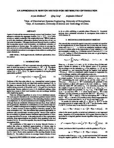
The simulation model is built according to the commercial bismuth telluride (Bi2Te3) TEG devices produced by Thermonamic Co. (TEP11264-3.4). The cubic polynomial functions of TE parameters tabulated in Table 1 are employed in the simulation which are fitted based on the temperature-dependent material parameters obtained from the manufacturer [26]. The TEM has a 40 mm × 40 mm dimensions. It consists of 126 pairs of p- and n-type Bi2Te3 legs connected electrically in series by soldering onto aluminum electrodes and thermally in parallel, as depicted in Fig. 1. The connecting bridges inside the modules are made of aluminum on both sides and act as electrodes. The ceramic plates enclosing the module are made of aluminum oxide. The external surfaces of the modules are covered with a thin layer of graphite to reduce the thermal resistance. The geometric parameters and properties of the model are determined by direct measurements or from other literatures which are listed in Table 2 for a TEG couple. Contact resistances including thermal and electrical contact resistances are recognized to have a significant impact on TEG performance, especially in the circumstances of large current or temperature differences. In this simulation, electrical contact resistances on both sides of the TE pellets and thermal contact resistances between the ceramic plates and Al electrodes are all considered. The electrical and thermal contact resistances are assumed to be the same on the both sides of p/n materials and temperature-independent. The regression analysis between the simulated data and measured data has been adopted to estimate the contact resistances precisely and the identified thermal and electrical contact resistances are 2.0 × 10−4 m2·K·W−1 and 6.5 × 10−9 Ω·m2 respectively [26]. In practice, Rc is implemented in the simulation by supplying a surface impedance ρs of the corresponding thin layer, which results in a jump in electrical potential by applying Eq. (4), where the subscripts 1 and 2 denote the two sides of the thin layer. As for rcont, it is implemented by supplying the thermal conductance h at their interface of two contacted components, for instance, subtracts and electrodes of TEMs. Correspondingly, a temperature difference is formed by applying Eq. (5), where the subscripts u and

2.1. Governing equations The TEG contains three TE effects: the Seebeck effect, Peltier effect, and Thomson effect [24]. The Seebeck effect (S·ΔT) refers to an electrical potential generated owing to a temperature difference between the joints of two dissimilar TE materials. The Peltier effect (S·T·I) is reversed of the Seebeck effect. It describes the heat absorbed or emitted at an electrified junction between TE materials and electrodes when a current I passes through the junction. The Thomson effect (TdS/ dT·I·∇T ) is a continuous version of the Peltier effect and it depicts the heat absorbed or emitted of a current-carrying TE material with a Table 1 The cubic polynomial functions of TE properties. Properties

Polynomial expressions

Sp

− 2.24407 × 10−11T3 + 2.22834 × 10−8T2 − 7.301 × 10−6T + 1.023698 × 10−3 (V/K)

λp

− 5.82609 × 10−8T3 + 1.03491 × 10−4T2 − 0.05011T + 8.726 (W/mK)

ρp

− 7.75456 × 10−13T3 + 7.77051 × 10

Sn

1.68178 × 10−11T3 − 1.77163 × 10−8T2 + 6.203 × 10−6T − 9.54589 × 10−4 (V/K)

λn ρn

− 6.04782 × 10−13T3 + 6.09155 × 10−10T2 − 1.715 × 10−7T + 2.11951 × 10−5 (Ω·m)

- 10T2

− 0.01853 × 10−5T + 1.60117 × 10−5 (Ω·m)

3.76869 × 10−9T3 + 2.81722 × 10−5T2 − 0.02057T + 5.09531 (W/mK)

586


H. He et al.

TE couple Ceramic plate Electrodes p-type TE leg

TEM

n-type TE leg External load Ceramic plate

External load Fig. 1. The schematic of a TEM (left) and a TE couple (right).

0.573 W for the heat flow rate while the NRMSEs become 2.06% and 1.96% respectively. It shows that there is little discrepancy less than 2.5% with regard to the heat rate and output power. This discrepancy is probably attributed to the incomplete equivalence of pre-set thermal boundary conditions of both models, which specifically results into a slight thermal difference of numerous constitute TE couples from its center to edges of the TEM. In view of its satisfactory consistent results, remarkable less calculation demand and time consumption (more than 95% time saved), the single model of a TEG couple is applied for analysis in the subsequent study. Furthermore, in order to explore the impacts of thermal and electrical contact resistance, Rc and rcont, a comparison based on TEG modeling with a constant 4 Ω load resistance applied is conducted under four different conditions with either, both and none of these two resistances considered. The simulated output power is depicted in Fig. 3 as follows. The comparison of curve 2 and 4 indicates that the introduction of rcont reduces the output power heavily by lowering its output current. And the comparison of curve 3 and 4 indicates that the introduction of Rc reduce the output power comparatively as well, which results from a lower temperature difference imposed on both ends of TE pellets. When both resistances are considered, its output power decreases by more than 50% according to curve 1 and 4. The simulation results demonstrate that the ignorance of contact resistance can result in a vast overestimation of TEG output, which proves to be a necessity for an accurate TEG modeling as well as its characterizing method.

d refer to the two contacted sides. An external resistance is connected with the simulation model as the load and its value can be adjusted as needed by assigning different resistivity allowing for its invariant dimensions.

n·J1 =

1 ρs (V2 − V1)

(4)

nd ·qd = h (Tu − Td )

(5)

2.3. Boundary conditions and initial settings The electrical potential boundary condition is set by ground connection of a cross section of the external load while the temperature boundary condition is set by keeping both sides of the module at a constant temperature. Generally, the wiring to connect the external load and real TEMs in practice is often thin and not short in length, resulting in a large thermal resistance and negligible heat conduction along the wiring. However, in the simulation the dimensions of the TEG model is restricted with a very short wiring for the sake of less computation demanding and time consumption. A constant temperature of the load is set at the ambient temperature 293.15 K and its interfaces are set as adiabatic conditions to avoid the error resulting from heat conduction along the short wiring. Special probes enable us to obtain TE variables. The current I is calculated by surface integration of the electric current density in one cross-sectional area while the heat flow is calculated by surface integration of the heat flux over the hot or cold side boundary area. A grid sensitivity analysis is performed to ensure grid independence in the simulation.

3. Experimental setup To obtain the performance of a TEM in terms of heat rate, electrical voltage and current under a wide range of temperature, contact pressure and external load conditions, a new simple symmetric test setup is designed to capture critical TE variables with high accuracy. The symmetric vertical structure of TEMs sandwiched around a thin ceramic plate heater is to reduce the measurement error of the heat flow and guarantee the reliability. On each side of the heater, an identical TEM and a heat sink is placed. Particularly, there lies one uniform-heating grooved copper plate accommodating thermocouples placed between the heater, heat sink and each TEM. The photo of the setup and the schematic diagram of the symmetric main body are shown in Fig. 4. The temperature of the hot side is precisely controlled by a programmable proportional–integral–differential (PID) temperature controller with a temperature stability of ± 0.1 K, which can set different multiple temperature setpoints. A linear temperature rises or declines between two

2.4. Comparison of two thermoelectric models at different scales In order to evaluate two TEG models in terms of efficiency and accuracy, a whole TEG model consisting of 126 pairs of p/n legs and a single model of one pair of p/n leg are modeled respectively as shown in Fig. 1. Accordingly, the comparison is conducted with the voltage and heat flow data scaled up by a factor 126 for the latter model in the same operating conditions. The data deviation can be evaluated through the root mean square error (RMSE) while normalized rootmean-square error (NRMSE) facilitates the comparison with different scales. In Fig. 2, the RMSEs are 0.021 W for the power output and 0.641 W for the heat flow rate in the case of 4 Ω. The corresponding NRMSEs are 2.37% and 2.44% respectively. When the external load resistance is 8 Ω, the RMSEs are 0.020 W for the power output and Table 2 The geometric parameters and properties of the model. Element

Electrical Conductivity (S/m)

Thermal Conductivity (W/(mK))

Size along x, y, z axis (mm)

Ceramic plate p-Bi2Te3

NA 1/ ρp (T )

36 [25] λp (T )

4.72 × 2.5 × 0.86 1.5 × 1.5 × 1.96

n-Bi2Te3

1/ ρn (T ) 3 × 107 3 × 107

λn (T ) 238 238

1.5 × 1.5 × 1.96

Upper Al electrode Lower Al electrode

587

4 × 1.7 × 0.6 2 × 1.7 × 0.34


H. He et al.

Output Power(W)

2.5 2.0

80

(a) 4ȍ TEM model TE couple model

4ȍ TEM model TE couple model

60

8ȍ TEM model TE couple model

1.5

(b)

70

Heat flow(W)

3.0

1.0

8ȍ

50

TEM model TE couple model

40 30 20

0.5

10

0.0 0

20

40

60 80 100 120 Temperature difference(K)

140

0

160

0

20

40


140

160

Fig. 2. Comparison of the simulated results by a complete TEG model consisting of 126 TE couples and a simplified model of a single TE couple.

7 6

Output Power(W)

thermal resistance in the interfaces between module and heater or heat sink, which guarantees firm bond and good reproducibility. Two identical TEMs operate in the same conditions and their similar test data indicates that both modules give identical performance for the same temperature difference. The deviation of outputs of two modules are less than 2%. The test results given in this paper are the average value from both modules. The greatest difficulty lies in the accurate measurement of the heat flow rate supplied to the TEM. In [28], the heat flow was measured based on the temperature gradient produced in a metal block of known thermal conductivity. By introducing a borosilicate or glass ceramic reference material with known thermal conductivity placed next to the TEM, the heat flow rate was obtained [29]. The heat flow can be then estimated indirectly by means of measuring the temperature difference at two specific sampled material locations. However, its main challenge for a precise measurement is the rational design of the reference block. The deviation can be ascribed to the non-ignorable heat losses from the side surface of a thick reference block, or the systematic errors from uncertainty of its thermal conductivity, temperature measurements as well as the determination of thermocouple’s exact installation sites for the block. Therefore, in view of an easy manipulation and high accuracy for heat flow measurement, it is estimated by measuring the power dissipation of the electrical heater [30]. To ensure that almost all the heat energy generated by electrical heater 1 is equally transferred to both TEMs symmetrically placed at its both sides, the heater is designed to be as thin as possible. The dimension of its cross section keeps the same with that of TEM. The heater is made from a good heat-

1 Both rcont and Rc considered 2 Only rcont considered 3 Only Rc considered 4 Neither rcont nor Rc considered

5 4 3 2 1 0

0

20

40


140

160

Fig. 3. Comparison of the simulated results in terms of contact resistances.

adjacent temperature setpoints in a given time interval can be achieved through an automated PID algorithm. Two aluminum heat sinks are connected to a circulating thermostatic water bath SLDCW-0510-II produced by ShunLiu Instrument to cool the cold side of TEGs. An electronic load, IT8511A+ (ITECH Electronic, USA) is connected to a TEM, which allows for a variety of loads to be performed [27]. A PANTHER air compressor and an air cylinder (SDA63x55, AIRTAC) are used to apply a horizontal clamping pressure to the TEM to minimize

(a)

(b) 4 23 5

PID Main Body Air Compressor Controller

Electronic UPS Load Data Acquisition Unit

9

8

10

61 7

Thermosat Fig. 4. (a) Photograph of the setup (b) Schematic diagram of the main body: 1—electrical heater; 2, 3, 4, 5—copper plate; 6, 7—TEM; 8, 9—heat sink; 10—air cylinder. 588


H. He et al.

The novelty of this test system lies in these aspects. First, in general, the device is simple in structure, small in size, low in cost and easy in implementation. Second, specifically, to avoid the impacts on the test results from other evitable factors, a vertical structure is designed to prevent the interference on clamp pressure affected by the clamp device’s own gravity. The thermal insulation material aluminosilicate fiber cotton is used to wrap the setup on its sides to reduce the heat loss. Third, the setup shows flexibility in terms of multi-parameters adjustment, such as surface temperatures of the TEM, the heat flow rate, external load and the clamp pressure. Fourth, its measurement is comprehensive and accurate. The grooves are designed in copper plates to accommodate multiple thermocouples at each interface, which verifies a small deviation of temperature measurement less than 2% to reduce it uncertainty. Moreover, a thin ceramic heater with a closely meandering heater wire is specially designed to realize the heat conduction of high power but reduction of heat loss on its side surfaces. In brief, the novelty lies in its simple structure, flexible control of multiparameters and accurate measurement. The test and model results at identical operating conditions are compared in Fig. 8 including the output voltage, current and heat flow at TEM’s hot side versus the temperature difference. The temperature of the thermostatic water bath keeps constant. Three tests are conducted at steady state for different load resistances: infinity (open-circuit), 6 Ω and zero (short-circuit) conditions. For the first case, the RMSEs are 0.020 V for the open-circuit output voltage and 3.78 W for the heat flow rate QH at the hot side of TEMs while the corresponding NRMSEs are 0.48% and 12.6% respectively. For the second case, the RMSEs are 0.037 V for the output voltage, 0.008A for the current and 4.514 W for QH. The corresponding NRMSEs are 1.63%, 1.79% and 12.1% respectively. For the third case, the RMSEs is 0.009A for the short-circuit current and 3.65 W for QH while the corresponding NRMSEs are 1.79% and 9.42% respectively. The simulated and measured voltage and current has a NRMSE less than 2% at all the applied load conditions, which indicates that the model is capable of precisely predicting electrical properties of TEMs. Nonetheless, the heat flow rate QH has a NRMSE ranging from 9.42% to12.6%. This deviation mainly results from the overestimation of the real QH by assuming that the electrical power of heater all converts to the heat flow through the TEMs. In practice, there exist inevitable heat losses due to radiation, convection and conduction through the flanks of the heater or along the power lines. According to multiple measurements, the uncertainty of measured voltage and current is within ± 2% while that of measured heat flow rate is considered as ± 5%. Overall, the simulated results show good agreement with

conducting ceramic plate with a closely meandering heater wire in it and can deliver heat of high power up to 330 W compared with usual thin heating films. Besides, the thermal insulation material aluminosilicate fiber cotton is used to shield the heater, which fills its flanks. An uninterrupted power supply (UPS) is used as the stabilized power supply (220VAC ± 1%, 50 Hz) located away from the heat source. The real-time voltage and current of the heater are respectively determined with two measured voltages across it and a shunt resistor recorded by Fluke 2438A Data Acquisition Unit. The PID controller adjust the electrical power delivered to heater by changing the duty cycle of solidstate relays connected to the heater, so a pulse voltage is actually exerted to the heater. Since the power frequency is much higher than the switching frequency (< 2 Hz) of PID controller, the rms voltage is preferred to estimate the thermal power of the heater with different duty cycles for diverse temperatures of the hot side, as described in Fig. 5. Thus the heat flow provided to each TEM can be defined as

QH =

1 1 PW D ·Uh Ih = Uh Ih 2 2 T

(6)

where Uh and Ih are the rms voltage and current of the heater respectively, D is the duty cycle, T is a time period including plenty of on-andoff cycles and PW is the pulse width (pulse active time) in the period. PW and T of input pulse voltage are also sampled by the Fluke 2438A Data Acquisition Unit. Another major error stems from the measurement of the TEM’s surface temperature, which is caused by uncertainties in the location of measuring sites and calibration of thermocouples. To address this issue, each TEM is placed between two grooved thin copper plates, and two shallow grooves are designed on its side attached to the TEM to accommodate K-thermocouples with a diameter of 0.1 mm and a precision of ± 1.1 K, as Fig. 6 depicts. All the eight channels of temperature data are collected by the Fluke 2438A Data Acquisition Unit. The extra carbon sheets are used to keep good thermal contact between interfaces of all parts. The acquisition of electric signals such as output voltage and current are much easier compared with those of heat flow rate and temperature. The load resistance along with its voltage and current are simultaneously and automatically recorded by the computer software NI1900. The clamping pressure also has a significant effect on the TEM performance due to its affected contact thermal resistance. The pressure unit composed of an air compressor and an air cylinder is also involved in this test apparatus. It makes sense to optimize the pressure by exploring the relation between the output power of TEM and the clamping pressure on the module. The above mentioned commercial Bi2Te3 TE devices TEP1-1264-3.4 are adopted. Results are presented in Fig. 7 for five different pressures of air compressor (0.1 MPa, 0.2 MPa, 0.4 MPa, 0.6 MPa and 0.7 MPa) for the TEM connected with a 6Ωload resistance at variable temperature differences of both sides of TEM. It indicates that the output power keeps rising with the increase of pressure for each working condition. The impact of the clamping pressure on output power is tremendous in case of a small temperature difference and decreases as the temperature difference enlarges. However, the deviation of the output powers at 0.7 MPa and 0.1 MPa still reaches 31.4% when the temperature difference is 137 K. Given a certain temperature difference, the growth rate of the output power slows down with the increase of pressure. When the clamping pressure increases from 0.1 MPa to 0.7 MPa, the RMSE for the output power between two adjacent pressure are respectively 0.158 W, 0.115 W, 0.090 W and 0.009 W while the corresponding NRMSE are 23.7%, 15.0%, 10.7% and 1.12%. vividly, the output power tends to be stable with a increasing clamping pressure. As a result, once the pressure reaches 0.6 MPa or above, the output power is deemed to be independent of pressure. Considering that a much higher clamping force will raise the risk of damage to TEG modules, all the tests below are performed at a constant air compressor pressure of 0.6 MPa.

(a) Th=323.15K

Pulse voltage(V)

216

0 0

3

6

Time(s)

9

12

15

9

12

15

(b) Th=423.15K

Pulse voltage(V)

216

0 0

3

6

Time(s)

Fig. 5. The pulse voltage supplied to the heater for different temperatures at the hot side of TEM. 589


H. He et al.

(a)

10

Open circuit Measured Simulated Simulated(|ĭp|=|ĭn|) 6ȍ Measured Simulated Simulated(|ĭp|=|ĭn|)

Voltage(V)

8

Fig. 6. A copper plate with two grooves on its surface attached to the TEM to accommodate thermocouples.

0

0

1.8 1.6

1.0

1.4 1.2

Current(A)

Output power(W)

1.5

4

2

0.1MPa 0.2MPa 0.4MPa 0.6MPa 0.7MPa

2.0

6

0.5

0.0 0

1.0

20

40

60 80 100 120 140 Temperature difference(K)

160

180

160

180

(b) Short circuit Measured Simulated Simulated(|ĭp|=|ĭn|) 6ȍ Measured Simulated Simulated(|ĭp|=|ĭn|)

0.8 0.6

20

40

60 80 100 Temerature difference(K)

120

140

0.4 0.2

Fig. 7. The output power of TEG versus temperature and the clamping pressure.

0.0 0

experimental data, verifying the effectiveness of the numerical model and the feasibility of the test device including its control and measurement systems.

120

4. Characterization methodology 100

Heat flow rate(W)

TE physical parameters are of great importance to quantify TEG performance and optimize its design but seldom offered by manufacturers. In order to obtain the temperature-dependent parameters including S, λ, ρ quickly and accurately, a novel approach for modules characterization called QSS method is first proposed. In this method, TE parameters at different temperatures are precisely obtained by measuring all TEG’s outputs, temperatures and heat flow rates, respectively in open and short circuit state. Meanwhile, irreversible effects including thermal and electrical contact resistances are all considered. The specific QSS method is described below in detail.

80

20

40


(c) Open circuit 6ȍ Measured Simulated Simulated(|ĭp|=|ĭn|)

Measured Simulated Simulated(|ĭp|=|ĭn|)

Short circuit Measured Simulated Simulated(|ĭp|=|ĭn|)

60 40 20

4.1. Assumptions and basic principle 0

Several certain reasonable assumptions are made to simplify the characterization model without too much deviation from the real conditions.

0

20

40


160

180

Fig. 8. Comparison of test and simulated results in identical operating conditions.

(a) The heat flows through a TEM along with its legs are assumed to be one-dimensional. (b) With regard to p- and n-type TE leg, they are assumed to share the same value of the thermal conductivity λ and electrical resistivity ρ but the same absolute value of Seebeck coefficient S with a right opposite polarity. (c) The Thomson effects and the heat leakage through the air zones within the TEM are ignored in the parameters solving process [31].

To address the second assumption, it is necessary to account for its feasibility in advance. Since commercial TEMs always have sandwich structures with all (p- and n-type) TE pellets connected electrically in series and thermally in parallel, objectively it is impossible to distinguish these two materials depending on the external output and parameters of TEMs. Therefore, the uniform constant TE properties shared by p- and n-type materials are always assumed by existing methods. As 590


H. He et al.

number of elements is N and the length of element i is denoted by δNi . The temperatures of its hot and cold side are Ti and Ti−1 while their i i i and QN,L . Apparently, QN,H and corresponding local heat flows are QN,H i−1 i i+1 QN,L are respectively equal to QN,L and QN,H . Each element has a small certain fixed temperature interval but with the same temperature difference ΔT. For each element the TE properties are assumed constant but vary for the other one. The local energy balance for element i is described by

for the QSS method, a uniform but temperature-dependent TE properties Φ(T) (S, λ and ρ) shared by them are assumed. Thus it is necessary to discuss and assess this assumption with regards to the TEG modeling. A comparison is implemented based on TEG modeling with real separate TE properties(Φp′ and Φn′) for both pellets and a unified average TE properties (|Φp| = |Φn| = (|Φp′| + |Φn′|)/2) respectively, as shown in Fig. 8. A little discrepancy between both simulation results with different loads applied validates the feasibility of the aforementioned assumption. Specifically, the NRMSE based on two results are all less than 1.2% for the voltage, current and heat flow rate. On account of the symmetrical structure of each TE couple, both its legs share the same heat transfer equation and temperature distribution allowing for an equal divided Peltier heat assumed as well as their uniform TE parameters λ and ρ. Therefore, only half a couple is focused for investigation as depicted in Fig. 9. Th, Tc, Qh and Qc denote the temperatures at the hot and cold side of the couple as well as their local heat flow respectively, which are directly determined by tests. TH, TL, QH and QL are the corresponding variables at both sides of the TE leg accordingly. Between each side of the substrate and its corresponding side of the TE leg, a total thermal resistance R (RH and RL for the hot and cold end respectively) generally consists of three parts: the thermal resistance of the ceramic substrate Rs and that of the electrode Re as well as thermal contact resistance Rc. An overall value Rc is adopted without separately considering those existing at both interfaces between substrate, electrode and TE leg. Besides, the electrical contact resistance rcont at the interface between the electrode and the TE leg is introduced instead of an actual solder layer with negligible thickness, where the temperature continuity is assumed. TH and TL can be determined by Eq. (7) and (8):

TH = Th − Q h RH

(7)

TL = Tc + Qc RL

(8)

ρ ∂ ∂T (λA ) + I 2 = 0 A ∂x ∂x

where A is the cross area of the TE leg. By solving the above second order differential equation for the general solution formula subjected to its boundary conditions at both extremities (x = 0, T=TLi , Q = QLi and x = δNi , T = THi , Q = QHi ), the Eqs. (18) and (19) for element i can be acquired while its spatial length is expressed by Eq. (14): i i QN,H = QN,L −

T i = T i−1 −

δNi =

(9)

QL = Qc − SL ITL − I 2rcont

(10)

Q h − Qc = I 2r load

(11)

Vload =

∫T

TH

L

2S (T ) dT − I (2rcont + r leg )

Si =

λi =

Since the data used to characterize by the QSS method are based on a single TE leg, while the measured data are based on the whole TEG which contains several legs, therefore the measured data need to be scaled down for calculation. In consideration of the periodic arrangement of TE couples with equivalent characteristics for each leg, some measured data for a TEM are regarded as 2•Nc times of those of a single TE leg such as output voltage Vm, heat flow rate Qmh, Qmc and load resistance, while other data are deemed to be equal to those of a single TE leg such as current Im, as described by Eq. (13)–(16), where Nc and the subscript m denote the number of TE couples for a TEM and the measured data respectively. (13)

Qmh = 2Nc ·Qh

(14)

Qmc = 2Nc ·Qc

(15)

Im = I

(16)

(18)

i QN,L δNi I 2ρi δNi2 + 2 i i 2λ A λA

i A (QN,L −

(19)

i2 QN,L − 2I 2ρi λi ·ΔT )

I 2ρi

(20)

For element i, both its Seebeck coefficient S and thermal conductivity λi are obtained in open circuit tests for simplicity with a constant conductive heat flow and no Joule heat and Peltier heat considered. Si between Ti−1 and Ti can be determined by Eq. (21) while λi is i through element i keeps given by Eq. (22) because the heat flow QN,H constant. Therefore, the solving of its electrical potential Vi and length δNi are the prerequisites for both TE parameters. Similarly, its electrical resistivity ρi can be deduced by Eq. (23) based on short circuit tests by applying the circuit theory and energy conservation law. This equation is only applicable to the case when all the variables (temperatures, heat flow, spatial lengths et al) of other elements except element i are solved as a premise. As a consequence, a progressive algorithm proposed for these variables are detailedly introduced in Section 4.2. Ii and Vi indicate the current and total electrical potential of the TE leg with respect to the unsolved element i.

(12)

Vm = 2Nc·V

I 2ρi δNi A

i

By introducing the one-dimensional heat conduction theory, Peltier and Seebeck effects, its internal relations to describe the characters of the TE leg are given by Eq. (9)–(12), where the subscripts h, c, H, L denote the hot and cold side of the couple as well as both sides of the TE leg respectively. rload, Vload and rleg are external load resistance, output voltage and resistance of a TE leg.

QH = Q h − SH ITH + I 2rcont

(17)

Vi ΔT

(21)

i QN,H ·δNi

(22)

A·ΔT

Qh

Rc

Th

Ceramic Substrate

Rs

Electrode

Re QH

N-type leg

TH

P-type leg

rcont

QL Electrode

TL

Electrode Ceramic Substrate Tc

Fig. 9. The schematic of half a TE couple. 591

Re Rs

Qc

In order to explore the thermal dependence of TE parameters, the TE leg is divided into several serial elements based on its inner temperature distribution, as shown in Fig. 10. For example, the total

RH

Rc

RL


H. He et al.

hot side

i i 1 QN,H (QN,L )

H(mm)

T i + 1 − T i = ΔT

Ti

(m ⩽ i ⩽ N− 1)

(24)

element N

4.3. Characterization algorithm in open circuit condition įNi

element i

element 1 cold side

įNi

TL

T

T

2

3

T

i-1

T

Ti

T(K)

ǻT 1

element i

i

T

TH

i N,L

i 1 N,H

Q (Q

To get rid of the impacts of Joule heat and Peltier heat for simplicity, the QSS method is implemented to get Seebeck coefficient and thermal conductivity based on the open circuit test. For the case with only one element at t = t1, the Seebeck coefficient S1 and thermal conductivity λ1 can be computed as:

1

)

S1 =

V1 ΔT1

λ1 =

QH·δ11 A·ΔT1

Fig. 10. Physical model of element i.

ρi δ i Ii2· = Ii Vi − Ii2 (2rcont + A

i−1

∑ j=1

δ jρ j ) A

(23)

(25)

(26) 1

δ11

At this point, V is equal to the Vload and is equal to the length l of the TE leg. Hereby the load resistance rlaod is recognized as infinity and Vload denotes actually the electrical potential of the TE leg. It is noted that QH flowing through the TE leg keeps identical at any horizontal cross-section in the open circuit condition all the time. Besides, the time-variant QH can be obtained directly by tests. When TH rises to T2, the TE leg is divided into two elements and the parameters S2 and λ2 for element 2 can be computed by Eq. (27) and (29). Its corresponding spatial length δ22 is given by Eq. (28). Apparently δ22 can be determined by subtracting δ21 from l.

4.2. Characterization procedures As previously described, it becomes a crucial issue to solve all the parameters of each TE element with high accuracy and efficiency, especially in the scenario of a large temperature range. To address this issue, a novel characterization principle called QSS method is put forward. As the name implies, the TEM is supposed to work in an opportune time scale between transient and steady state. Its thermal condition varies slowly and its real-time performance is in close proximity to that of steady state. Utilizing the test setup in Section 3, a flexible adjustment of the TEM’s thermal conditions for QSS method is easy to carry out. The heating process is precisely controlled by the programmable PID controller by setting its initial value T0, final value Ts and heating time Δt, thus Th rises continuously at a certain preset rate. During this period, the thermostatic water bath is set to a fixed temperature of 278.15 K (5 °C) as the chiller to cool the cold side of the TEG. In practice, when a larger heat flow rate Qh arises from a higher Th, Tc is gradually raised due to its limited cooling capacity of the chiller as well as the invariant heat resistance of the heat sink and its inevitable thermal contact resistance. The temperature variation of both sides of the TE leg is schematically depicted in Fig. 11. All the experimental data are sampled and recorded in real time in terms of Qh, Th, Tc, I and V. Two independent tests are conducted corresponding to the open and short circuit condition respectively. For both tests, the heater is programmed for the same heating process while the thermostatic water bath is set to a fixed cooling temperature. The temperature dependent parameters S(T), λ(T) are derived by the open circuit test and ρ(T) by the short circuit test. The detailed segmentation method during the test period can be illustrated in Fig. 12. It is noted that the concerned boundary temperatures are TH and TL, which can be calculated by solving Eq. (7), (8) and (11). Before TH rises to T1, the whole TE leg is regarded as one element, i.e., it shares the same physical parameter. Once TH rises to T1 at t = t1, the temperature difference of both sides is ΔT1. Then TH keeps rising until it reaches to T2 at t = t2. Hereby the TE leg is divided as two adjacent elements with their interface lying at T = T1, where the heat 1 2 flow rate is Q2,L or Q2,H . The subscripted number denotes the present total number of divided elements and the superscripted one denotes its sequence number of the present element. The temperature TL rises 1 1 slowly from T1,L to T2,L . Their temperature differences for the two elements are ΔT2 and ΔT and their spatial length are δ21 and δ22 correspondingly. For element i, it has a set of constant physical parameter including Si, λi and ρi. The continuously rising temperature TH reaches to TN at t = tN finally and TL rises to TN1 −m + 1,L , which is right between Tm−1 and Tm. The TE leg is therefore divided into N-m + 1 elements. The temperature at their interfaces is Ti, as defined by Eq. (24). The temperature difference for these N-m elements is ΔT, while it is ΔTN for the one left in the cold side.

S2 =

V2 − S1ΔT2 ΔT

(27)

λ1AΔT2 QH

(28)

δ22 = l −

λ2 =

QH·δ22 A·ΔT

(29)

In the same way, once TH reaches to T , the parameters S and λN for element N can be derived by Eq. (30)–(32), which corresponds to the temperature interval between TN−1 and TN. Herein the variables Si and λi (1 ≤ i ≤ N) are all obtained, forming the temperature dependent TE physical parameters S(T) and λ(T). N

N

N −1

SN =

VN − ∑i = m + 1 S i ΔT − S mΔTN N −1

δNN−−mm++11 = l −

∑ i=m+1

λN =

(30)

ΔT λi

AΔT AΔTN − λm QH QH

(31)

QH·δNN−−mm++11 A·ΔT

(32)

TH

TN

TL

Temperature(K)

TN-1 TN-2

T2 T

TN-1 m +1,L TN-1 m -1,L

1

T0

t1

t2

tN-2

Time(min)

tN-1

tN

1 T1,L

Fig. 11. The schematic diagram of the temperature variation of the TE leg based on the QSS characterization method. 592


H. He et al. 1 T 1 (TH ), Q1,H (QH )

2 T 2 (TH ), Q2,H (QH )

į22

į11

S1, Ȝ1, ȡ1

2

2

S ,Ȝ,ȡ

į

N-m 1 T N (TH ), QNm +1,H (QH )

N-m 1 N-m 1

N

N

S ,Ȝ ,ȡ

T N-m 1 N-m T N 1 , QNm +1,L (QN-m +1,H )

N

T

2

2 T 1 , Q2,L (Q21,H )

T1

į21

S1, Ȝ1, ȡ1

1 1 T1,L (TL ), Q1,L (QL )

į

T2

1 įN-m

1 1 T2,L (TL ), Q2,L (QL )

t=t1

2 N-m 1

m+1

S

m+1

,Ȝ

,ȡ

3 2 T m 1 , QNm +1,L (QN-m +1,H ) T 2 1 T m , QNm +1,L (QN-m +1,H ) TN 1 TN-1 m +1,L (TL ), QNm +1,L (QL )

m+1

Sm, Ȝm, ȡm

1

t=t2

t=tN

Fig. 12. Scheme of the TE leg segmentation according to the QSS characterization method.

short circuit tests, resulting in the varying heat flow versus spatial coordinates of TE leg at any time. When TH rises to T1, ρ1 is given by

4.4. Characterization algorithm in short circuit condition The acquisition method of its electrical resistivity ρ(T) is mostly similar to those of S(T) and λ(T) and even more complex in some aspects. The intractability stems from the nonnegligible Joule heat in

ρ1 =

(S1ΔT − 2I1 rcont )·A l·I1

(33)

Start

Input Iload, TH, TL, QH, QL of the short-circuit test.

Prepare the measurement system for temperature, heat flow and related electrical parameters sampling. Supply the clamping pressure 0.6MPa.

Given i=1 Calculate ȡ1 by Eqs. (27)

Set a fixed temperature of the thermostatic water bath and T0, Ts, ǻt of the PID controller

i=i+1

Conduct two tests in open-circuit and short-circuit conditions in sequence respectively.

Assume TL is between Tk-1 and Tk, (1 k i).

Calculate the time-variant TH, TL, QH and QL by Eqs. (5)-(9) for both tests.

1 Calculate Qi k

1,L

by Eqs. (7)-(9)

Given j=1

Input Vload, TH, TL, QH, QL of the open-circuit test. Given i=1

Qi j k1 1,L

Calculate S1 and Ȝ1 by Eqs. (19)-(20)

įi j k1 1

A(Qi j k1 1,L

Qi j k

I j 2 ȡ j įi j k 1,L

2

Ij ȡ

Vi

k 1 k 1

l

i 1 j k 1

S ǻT

k

i).

S ǻTi

Ȝj

AǻT QH

ǻT AǻTi Ȝk Ȝi QH ,

įii

i=N ?

2

QH įii kk 11 AǻT

ǻT )

No

j=j+1

Yes

k

j k 1

Si įii

j

k

j k

j=i-k-1? i 1

,

Qi j k1 1,L 2 2 I i 2 ȡ j k Ȝ j

i=i+1 Assume TL is between Tk-1 and Tk, (1

1

A

i i k 1 i k 1

Ii ȡ į A

Ii (

i

k 1 k 1

l

i k q 1

įi j k 1 ,

S q ǻT +S k ǻTi ) I i 2 (2rcont

q k 1

q

i=N ?

No

No

Yes

Yes

Export S(T), Ȝ(T) and ȡ(T) Stop

Calculation by MATLAB

Fig. 13. Flowchart of the characterization procedure based on the QSS method. 593

įiq kk 11 ȡq ) A k

i 1


H. He et al.

where I1 denote the present electric current. Once TH rises to T2, the spatial length of both formed elements can be determined by Eq. (34) and (35). In consideration of the variant heat flow rate at each inter1 face, Q2,L (QL) has to be computed in advance by Eq. (9)–(11). Thus ρ2 can be deduced by Eq. (36) as follows:

A (Q2,1 L −

-4

Q2,12L − 2I22 ρ1λ1·ΔT2 )

3.5

I22 ρ1

δ21

δ22

=l−

I22

δ 1 ρ1 ρ2 δ22 = I2 (S1ΔT2 + S 2ΔT ) − I22 (2rcont + 2 ) A A

(36)

Similarly, it is noticed that the key to compute ρ for element N based on Eq. (40) is to figure out the spatial lengths of each element as a premise. Consequently, the spatial length of the other N-m elements and the heat flow through the interfaces between two adjacent elements are computed by iteratively solving Eq. (37) and (38) in case of the obtained QN1 - m + 1,L (QL) by Eq. (9)–(11). ρN is finally deduced by Eq. (39) and (40).

QNi +−1m + 1,L = QNi −m + 1,L − A (QNi +−1m + 1, L

IN2 ρi δNi −m + 1 A

−

(1 ⩽ i ⩽ N− m − 1)

QNi +−12 m + 1, L − Ii2 ρi + m

2.5

2.0

300

320

(38)

N −1

∑ q=m

380

400

420

440

420

440

420

440

×10

(b) (39)

IN2 ρ N δNN−−mm++11 = IN ( ∑ S qΔT +S mΔTN ) − IN2 (2rcont + A q=m+1

360

-5

δNq−m + 1

q=1

340

Temperature(K)

3.0

N

280

2IN2 ρi + m λi + m ·ΔT )

Data derived from test (ǻT=4K) Data derived from test (ǻT=8K) Data derived from test (ǻT=12K) Data derived from simulation Data from manufacturer

2.5

m+1 q δNq−−m +1 ρ ) A

Electrical resistivity(ȍ•m)

∑

3.0

1.5

(37)

N −m

δNN−−mm++11 = l −


(35)

N

δNi +−1m + 1 =

×10

(a)

(34)

Seebeck coefficient(V/K)

δ21 =

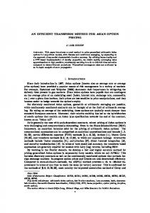
electrical resistivity. And the corresponding NRMSEs are 0.226%, 0.261% and 2.00% for Seebeck coefficient, thermal conductivity and electrical resistivity, respectively. Their good consistence verifies its feasibility and accuracy of the QSS characterization method.

(40) In this way, all three temperature-dependent parameters S(T), λ(T) and ρ(T) are obtained. Furthermore, the MATLAB program is utilized to solve the above equations efficiently and precisely. The flow chart of TEG characterization procedure based on the QSS method is described in Fig. 13. The bold variables in this flow chart stands for an array of test data in practice.

2.0 1.5 1.0 0.5

5. Validation and discussion

0.0

280

300

320

340

360

380

400

Temperature(K)

Firstly, validation of the QSS method is intentionally performed with its original input data from simulation TEMs to eliminate the impacts of data uncertainty. Then its practicability is explored with the measured data based on the test rig in Section 3. The effects of heating rate of tested TEM’s hot end temperature and the input sampled data at different time interval are also discussed. In addition, comparisons with other presented methods and limitations of the QSS method are illustrated to the last of this section.

3.5

(c)


-1

-1

Thermal conductivity(W·m K )

3.0

5.1. Validation by tests and simulations In order to validate the correctness of the novel QSS method proposed in Section 4, the aforementioned numerical TEG model is employed to work in short circuit and open circuit conditions at different temperature difference. Mass data including simulated TEG current, voltage and heat flow are sent to the interactive algorithm for temperature-dependent parameters calculation. The estimated data by simulation including S(T), λ(T) and ρ(T) are compared with those offered by the manufacturer, as shown in Fig. 14(a)–(c). For the latter, in each figure an average curve coming from both p-type and n-type data is supplied due to the assumption that both legs share the identical TE parameters. The RMSEs are 5.24e−07 V/K for Seebeck coefficient, 3.99e−3 W·m−1·K−1 for thermal conductivity and 2.39e−07 Ω·m for

2.5 2.0 1.5 1.0 0.5

280

300

320

340

360

380

400

Temperature(K) Fig. 14. The comparison of calculation TE parameters and those obtained from the manufacturer. 594


H. He et al.

dependent TE properties in a single pass, the other primary characterizing methods are generally put forward for constant TE properties in a specified temperature range. Thus an objective appraisement of them in terms of efficiency necessitates a quantitative comparison of measurement time duration Tm under a unified premise. Generally, Tm of reported methods [13] from more to less are the steady-state method, Gao Min method, Harman method and RSS method. For the first two methods, a considerable time consumption lies in the time allocation for their change in electrical load applied to the TEM especially under steady state condition. For Harman method, an inevitable time consumption to reach the initial steady state in case of a current applied to the TEM contributes to a considerable Tm with a typical referenced time of 2 × 675 s for two opposite polarities reported by Mahajan [16]. The RSS method can be implemented within several seconds allowing for its fast step change in 10 ms. As for the present QSS method, a constant TE properties are often assumed in a small temperature range with ΔT ≤ 8K. Its maximum Tm is estimated as 2 × 320 s for both open- and short-circuit conditions with a heating rate of 1.5 K/min, which is less than half of that of Harman method but more than that of RSS method. Nonetheless, the superiority of QSS method lies in the TE properties solving for different temperature ranges, which lasts for a time interval of 320 s between two successive ranges. As for RSS method, the Th and Tc have to be altered frequently and a comparative total Tm relies on a specific complex system while can realize a periodic scan of the electronic load with its data accurately interacted with the programable thermostat for the sake of automatic temperature alteration.

The rational implementation of the QSS TE characterization method depends on a suitable time interval selected for TEM heating to achieve a compromise between the time-saving and the steady state approximation. To determine the time interval and analyze its sensitivity, different heating duration 1 h, 2 h, 3 h and 4 h are set for the PID temperature controller with Th rising from 280.15 K to 464.15 K. The test is conducted in open circuit condition and both the output voltage Vload and heat flow Qh in its hot side versus temperature difference are shown in Fig. 15. The RMSEs are 0.098 V, 0.097 V and 0.116 V for the voltage output and 4.50 W, 1.51 W, 0.989 W for the heat flow rate accordingly when the case of 1 h, 2 h and 3 h are compared with that of 4 h. And the corresponding NRMSEs are 2.45% and 2.43% and 2.89% for the voltage and 13.3%, 4.45% and 2.91% for the heat flow rate respectively. All these four heating times Δt make little difference with regard to electrical output. However, the heat flow for the 1 h case is evidently larger than those of other cases. Once Δt is extended to 2 h or longer, the curves of test results have small fluctuation. More precisely, it means that the QSS method is independent of heating time once its rising rate of Th is less than 1.53 K/min in the tests. The heating time Δt is set as 2 h in the latter study. Furthermore, the appropriate selection of ΔT is another key issue for the QSS method. To explore its impacts, the obtained parameters S(T), λ(T) and ρ(T) based on the tests with different ΔT (4 K, 8 K and 12 K) are compared in Fig. 14(a)–(c). All these obtained results for each parameter generally match well with each other in these three cases. Nevertheless, a less ΔT stands for a more evident fluctuation of calculated data in case of a low temperature difference. It probably results from the measuring error in this specific condition. It is concluded that the selection of the optimal value of ΔT largely depends on the precision of test measurement. The calculated results based on tests are compared with manufacturer’s results to further validate its feasibility of the QSS method applied in the actual test setup in this paper. The RMSEs are 4.34e−06, 5.24e−6, 7.09e−6 V/K for Seebeck coefficient, 0.218, 0.193, 0.213 W·m−1·K−1 for thermal conductivity and 1.47e−06, 1.36e−6, 1.55e−6 Ω·m for electrical resistivity accordingly when the case of ΔT = 4 K , ΔT = 8 K and ΔT = 12 K are compared with the manufacturer’s data. And the corresponding NRMSEs are 1.87%, 2.26% and 3.06% for Seebeck coefficient and 14.4%, 12.6% and 13.9% for thermal conductivity and 12.1%, 11.4%, 13.1% for electrical resistivity respectively. Therefore, ΔT of 8 K is more advisable allowing for its smallest deviation in general. The peak errors exist either in the low or high temperature section. The relative error of temperature measurement is large in the low temperature section, while the relative of heat flow rate is large in the high temperature section. With respect to ρ(T), the error mainly comes from the overestimation of the short-circuit heat flow and thermal conductivity as well as the uncertainty of short-circuit current. Overall, the obtained parameters by the QSS method are in accordance with the reference data offered by the manufacturer. It indicates that the novel QSS method is reliable and appropriate to be applied with the specially designed setup in this paper. To further validate the QSS method and investigate whether the identified TE physical parameters also enable the accurate prediction of the TEG performance, the measurements and simulations are conducted by using another TEG device TEP1-1264-1.5 of the same TE materials. The third-order polynomial functions are adopted to fit these TE parameters obtained before. The TEG performance based on tests and simulation in same operating conditions is shown in Fig. 16. The RMSE is 0.147 V for the open-circuit voltage, 0.051A for the short-circuit current and 2.95 W for the heat flow rate. The corresponding NRMSEs are 4.61%, 5.28% and 7.17%. The acceptable consistent results indicate that the utilization of the QSS characterization method to determine the TE parameters and predict TEG performance is feasible and precise.

8

(a)

1h 2h 3h 4h

7

Voltage(V)

6 5 4 3 2 1 0

0

20

40

60

80

100

120

140

160

180

Temperature difference(K) 80

(b) 70

1h 2h 3h 4h

Heat flow rate(W)

60 50 40 30 20 10 0 0

20

40

60

80

100

120

140

160

180

Temperature difference(K)

5.2. Comparison with other methods

Fig. 15. The heating time Δt sensitivity analysis under open-circuit test condition.

Unlike the QSS method aiming at the acquisition of temperature595


H. He et al.

7 6

Open circuit Measured Simulated

5

Voltage(V)

TE properties. Moreover, the impacts of substrates and related contact resistances are often ignored by them but considered by QSS method. Its accuracy for TE properties is also validated by comparing the data derived from simulation and manufacture in Fig. 14. Nonetheless, the steady-state method, RSS method and QSS method all calls for a measurement of heat flow rate while both the Harman method and Gao Min method remove the need for it. The unachievable measurement in actual working conditions by the Harman method results in a higher difficulty and lower convenience for its implementation while the Gao Min method is sensitive to the fluctuation of the supplied heat flow rate. And the QSS method has its own limitation. By this method, the TE properties of a certain temperature interval are calculated based on the results of the previous temperature intervals. The measurement deviation is iterated at every step and easy to results in the error accumulation, which remains a challenge especially allowing for the larger uncertainty of measured heat flow rate at higher temperatures. A probable solution lies in the adoption of suitable referenced materials with known thermal conductivity, heat flux sensors as well as vacuum atmosphere for ignored heat leakage. In short, the presented QSS method acts as a competitive alternative in terms of efficiency, accuracy and practicability based on a premise of limited expense and volume occupied.

(a)

4 3 2 1 0

0

2.4


140

(b) Short-circuit Measured Simulated

2.0 1.6

Current(A)

20

6. Conclusions In this paper, the main works as followings is accomplished:

1.2

(1) A three-dimensional numerical model of TEG module is established with the COMSOL Multiphysics software. All TE effects including the Seebeck, Peltier and Thomson effects and Joule heating are considered, as well as the irreversible impacts from the subtract and contact resistances. The feasibility of modeling a single thermoelectric couple instead of a complete TEM is explored and confirmed for less calculation demanding and time-consuming purpose. (2) A novel symmetric test setup is designed to accurately acquire both the electrical and thermal variables of TEGs such as heat flow rates, voltages and currents at different temperature. The electrical load and clamping pressure can be adjusted flexibly. The performances of TEG modules based on tests and simulations in identical operating conditions are compared. The results show that both electrical outputs fit well with the NRMSE less than 2% while the heat flows are overestimated by 12.6% caused by the measurement uncertainty allowing for the inevitable heat losses. Overall, the simulated results show good agreement with experimental data, verifying the effectiveness of the numerical model and the feasibility of the test device including its control and measurement systems. (3) The most important innovation in this study lies in the novel characterization method called QSS method to fast and precisely calculate the temperature-dependence TE parameters (S(T), λ(T), ρ(T)). The characterization procedure is to raise Qh continuously in an appropriate time and keep the thermostat at a constant temperature in open and short circuit conditions in sequence. The TE leg is discretized in several serial elements according to their different temperature range. S(T) and λ(T) are directly calculated by open circuit tests and ρ(T) by short circuit tests. Meanwhile, contact thermal and electrical resistances are considered in the estimation. (4) The comparison of calculated thermoelectric parameters based on simulation and those from the manufacturer validates the correctness of the QSS method. The heating rate less than 1.5 K/min is preferred to achieve a compromise between the time-saving and the steady state approximation. The obtained TE parameters based on tests with different ΔT are compared to the manufacturer’s data to determine the optimal ΔT and both results agree well generally.

0.8 0.4 0.0

0

120


120

(c)

100

Open circuit Measured Simulated

80

Heat rate(W)

20

Short circuit Measured Simulated

60 40 20 0

0

20


140

Fig. 16. The TEG performance based on test and simulation in the same operating conditions.

In terms of accuracy, it contains two basic meanings: one indicates that the obtained TE properties assists an accurate TEG modeling and the other refers to the accurate obtained TE properties themselves. For the former, many literatures prove that an accurate TEG modeling necessitates the employment of temperature-dependent TE properties especially for a large current or temperature difference, which can be obtained by QSS method but hardly directly supplied by the other existing methods. For the latter, a significant discrepancy generally exists between the obtained constant values by existing methods and the real

The conclusions given in this study, particularly the QSS method to 596


H. He et al.

calculate the TE parameters, will provide guidance for the estimation of TEG performance and its optimization for large scale applications.

1007/s11664-014-3559-6. [14] Rauscher L, Fujimoto S, Kaibe HT, Sano S. Efficiency determination and general characterization of thermoelectric generators using an absolute measurement of the heat flow. Meas Sci Technol 2005;16:1054–60. https://doi.org/10.1088/09570233/16/5/002. [15] Montecucco A, Buckle J, Siviter J, Knox AR. A new test rig for accurate nonparametric measurement and characterization of thermoelectric generators. J Electron Mater 2013;42:1966–73. https://doi.org/10.1007/s11664-013-2484-4. [16] Mahajan SB. A Test setup for characterizing high- temperature thermoelectric modules [Master Thesis]. Rochester Institute of Technology; 2013. [17] Min G, Rowe DM. A novel principle allowing rapid and accurate measurement of a dimensionless thermoelectric figure of merit. Meas Sci Technol 2001. https://doi. org/10.1088/0957-0233/12/8/337. [18] Buist RJ. Methodology for testing thermoelectric materials and devices. In: Rowe DM, editor. CRC handbook of thermoelectrics. CRC Press; 1995. p. 189–96 (Chapter 18). [19] COMSOL 4.2 User Guide. Burlington, MA: COMSOL, Inc.; 2012. [20] Zhou S, Sammakia BG, White B, Borgesen P. Multiscale modeling of thermoelectric generators for the optimized conversion performance. Int J Heat Mass Transf 2013;62:435–44. https://doi.org/10.1016/j.ijheatmasstransfer.2013.03.014. [21] Seif S, Thundat T, Cadien K. Evaluation of efficiency factors and internal resistance of thermoelectric materials. Int J Energy Res 2017;41:198–206. https://doi.org/10. 1002/er.3584. [22] Siouane S, Jovanović S, Poure P. Fully electrical modeling of thermoelectric generators with contact thermal resistance under different operating conditions. J Electron Mater 2017;46:40–50. https://doi.org/10.1007/s11664-016-4930-6. [23] Ebling D, Jaegle M, Bartel M, Jacquot A, Böttner H. Multiphysics simulation of thermoelectric systems for comparison with experimental device performance. J Electron Mater 2009;38:1456–61. https://doi.org/10.1007/s11664-009-0825-0. [24] Hu X, Takazawa H, Nagase K, Ohta M, Yamamoto A. Three-dimensional finiteelement simulation for a thermoelectric generator module. J Electron Mater 2015;44:3637–45. https://doi.org/10.1007/s11664-015-3898-y. [25] Børset MT, Wilhelmsen Ø, Kjelstrup S, Burheim OS. Exploring the potential for waste heat recovery during metal casting with thermoelectric generators: On-site experiments and mathematical modeling. Energy 2017;118:865–75. https://doi. org/10.1016/j.energy.2016.10.109. [26] Högblom O, Andersson R. Analysis of thermoelectric generator performance by use of simulations and experiments. J Electron Mater 2014;43:2247–54. https://doi. org/10.1007/s11664-014-3020-x. [27] He W, Zhang G, Li G, Ji J. Analysis and discussion on the impact of non-uniform input heat flux on thermoelectric generator array. Energy Convers Manag 2015;98:268–74. https://doi.org/10.1016/j.enconman.2015.04.006. [28] Takazawa H, Obara H, Okada Y, Kobayashi K, Onishi T, Kajikawa T. Efficiency measurement of thermoelectric modules operating in the temperature difference of up to 550K. In: 2006 25th int conf thermoelectr; 2006. https://doi.org/10.1109/ ICT.2006.331330. [29] Sandoz-Rosado E, Stevens RJ. Experimental characterization of thermoelectric modules and comparison with theoretical models for power generation. J Electron Mater 2009;38:1239–44. https://doi.org/10.1007/s11664-009-0744-0. [30] Ciylan B, Yılmaz S. Design of a thermoelectric module test system using a novel test method. Int J Therm Sci 2007. https://doi.org/10.1016/j.ijthermalsci.2006.10.008. [31] Nemati A, Nami H, Yari M, Ranjbar F, Rashid Kolvir H. Development of an exergoeconomic model for analysis and multi-objective optimization of a thermoelectric heat pump. Energy Convers Manag 2016;130:1–13. https://doi.org/10. 1016/j.enconman.2016.10.045.

Acknowledgement This research is supported by the National Natural Science Foundation of China [grant number 51607135] and the China Postdoctoral Science Foundation [grant number 2017M613132]. References [1] Liu C, Deng YD, Wang XY, Liu X, Wang YP, Su CQ. Multi-objective optimization of heat exchanger in an automotive exhaust thermoelectric generator. Appl Therm Eng 2016;108:916–26. https://doi.org/10.1016/j.applthermaleng.2016.07.175. [2] He W, Wang S, Li Y, Zhao Y. Structural size optimization on an exhaust exchanger based on the fluid heat transfer and flow resistance characteristics applied to an automotive thermoelectric generator. Energy Convers Manag 2016;129:240–9. https://doi.org/10.1016/j.enconman.2016.10.032. [3] Sakdanuphab R, Sakulkalavek A. Design, empirical modelling and analysis of a waste-heat recovery system coupled to a traditional cooking stove. Energy Convers Manag 2017;139:182–93. https://doi.org/10.1016/j.enconman.2017.02.057. [4] O’Shaughnessy SM, Deasy MJ, Kinsella CE, Doyle JV, Robinson AJ. Small scale electricity generation from a portable biomass cookstove: prototype design and preliminary results. Appl Energy 2013;102:374–85. https://doi.org/10.1016/j. apenergy.2012.07.032. [5] Champier D, Bedecarrats JP, Rivaletto M, Strub F. Thermoelectric power generation from biomass cook stoves. Energy 2010;35:935–42. https://doi.org/10.1016/j. energy.2009.07.015. [6] Siviter J, Knox A, Buckle J, Montecucco A, McCulloch E. Megawatt scale energy recovery in the Rankine cycle. In: 2012 IEEE energy convers congr expo ECCE 2012; 2012. p. 1374–9. https://doi.org/10.1109/ECCE.2012.6342655. [7] Siviter J, Montecucco A, Knox A. Experimental application of thermoelectric devices to the rankine cycle. Energy Procedia 2015;75:627–32. https://doi.org/10.1016/j. egypro.2015.07.472. [8] Sundarraj P, Taylor RA, Banerjee D, Maity D, Roy SS. Experimental and theoretical analysis of a hybrid solar thermoelectric generator with forced convection cooling. J Phys D Appl Phys 2017;50:015501. https://doi.org/10.1088/1361-6463/50/1/ 015501. [9] Liu L, Lu XSen, Shi ML, Ma YK, Shi JY. Modeling of flat-plate solar thermoelectric generators for space applications. Sol Energy 2016;132:386–94. https://doi.org/10. 1016/j.solener.2016.03.028. [10] Ong KS, Naghavi MS, Lim C. Thermal and electrical performance of a hybrid design of a solar-thermoelectric system. Energy Convers Manag 2017;133:31–40. https:// doi.org/10.1016/j.enconman.2016.11.052. [11] Rahbar N, Asadi A. Solar intensity measurement using a thermoelectric module; experimental study and mathematical modeling. Energy Convers Manag 2016;129:344–53. https://doi.org/10.1016/j.enconman.2016.10.007. [12] Whalen SA, Dykhuizen RC. Thermoelectric energy harvesting from diurnal heat flow in the upper soil layer. Energy Convers Manag 2012;64:397–402. https://doi. org/10.1016/j.enconman.2012.06.015. [13] Pierce RD, Stevens RJ. Experimental comparison of thermoelectric module characterization methods. J Electron Mater 2015;44:1796–802. https://doi.org/10.

597