An Artificial Neural Network System for Trainborne Equipment BACC Signaling Recognition Alessio GAGGELLI, Stefano MANETTI, Alberto REATTI, Angelo Giuseppe VIOLI
Abstract—Neural networks recently gained attention as a fast and flexible modeling, simulation, and optimization tool in power electronics, signal processing as well in the pattern recognition field. Therefore, railway signaling recognition process candidate itself to an ideal task for a neural network based system. The aim of this contribution is to show an application of a feedforward neural network in the on board detection of control signals which are transmitted from the track-side plant to the train driver’s cab. A feedforward neural network receives the signal from magnetic sensors, decodes it even when it is affected by a high noise level, and generates the control command related to the recognized code. The network configuration has been determined by using an experimental approach. That is, several networks have been trained and tested and, finally, the neural network resulting in the highest performance/complexity ratio has been selected. The network has been trained and tested by using several signals and results in a low overall error. This communication shows that a neural network based identification circuit results in a faster execution speed, higher noise immunity, a much simpler, and a lower cost system tha n those used at present.
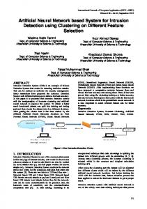
I. INTRODUCTION Neural networks are recently showing good promises for several applications such as microwave circuit design [1]-[6], power electronics [7]-[9], fault diagnosis [10]-[12] etc. So far they have been applied in these fields but their application in control and safety of railway systems is practically new. The Italian State railways system is based on the overall rail track division in several blocks, most of them 1350 meters long. As shown in Fig. 1, a signal generation system (BACC is the acronym for Blocco Automatico a Correnti Decodificate which means Codified Current Automatic Block) is placed at the beginning of each block. This system generates a numerical code, which
defines the block status. The signal is transmitted by using a single block rails as transmission line. Fig. 1 shows the signal current path constituted by the block rails and the train wheels set. Two sensors, installed under the train driver’s cab, detect the magnetic field generated by the current. The difference between the signals detected by each sensor is used to recognize the code related to the signal. This allows for a preliminary common mode noise reduction and emphasizes the useful signal.
Fig. 1 - Example of coded signal transmitted along the track.
The control signals considered in this work are transmitted and detected by using a 9 Codes Continuous Transmission Mode [13] and [14]. Table I shows these codes and their meaning. Frequencies f 1 and f 2 in Table I are related to two sinusoidal carriers at 50 Hz and 178 Hz transmitted along the block rails. The nine codes are generated modulating the carrier amplitude cyclically any minutes, e.g., code 270 is generating by setting to 0 the carrier amplitude 270 times in a minute as shown in Fig. 2(a). Fig. 2(b) shows a code obtained by superimposing the two 50 Hz and 178 Hz amplitude modulated carriers.
Table I. Nine Code System CODE
COMPOSITION
MEANING
270** 270* 270 180*
270 f1 +120 f2 270 f1 +75 f2 270 f1 180 f1 +75 f2
180
180 f1
120** 120* 120 75
120 f1 +80 f2 120 f1 +75 f2 120 f1 75 f1
Free running Stop signal at 5400 m Stop signal at 4050 m Speed reduction signal to 100/130 km/h at 2700 m or work in progress on the block – reduce the speed to 150 km/h. Notice of a stop signal or a speed reduction to 30/60 km/h at 2700 m Speed reduction signal to 130 km/h at 1350 m Speed reduction signal to 100 km/h at 1350 m Speed reduction signal to 30/60 km/h at 1350 m Stop
The purpose of this paper is to present a system for the signal identification based on a neural network built by using a low-cost microprocessors (Microchip series PIC). The neural network utilized for this system is a feed- forward multi- layer neural network, based on a continuous bipolar activation technique and supervised by an error back-propagation algorithm [15]-[17].
(a)
(b)
Fig. 2 - BACC code examples. (a) Code with 50 Hz carrier modulation. (b) Code with both 50 Hz and 178 Hz carriers modulation.
II. NEURAL NETWORK SELECTION AND TRAINING PROCEDURE The real time identification system has been studied, developed, and built on the basis of the following requirements: − fully compliance with the system currently utilized; − reliability of the decoded signals; − high noise rejection ratio; − cost reduction. The neural network analyzer operates with a digital signal obtained from the analog one by using a 1024 Hz sampling frequency and a 16 bit quantization. The 16 bit signal is then associated to an integer number corresponding to the numerical value of the sample. The neural network utilized in this paper has been implemented by using a computer algorithm NeuralNet developed by the authors, which has been written by using the C++ programming language resulting in a reliable, versatile and easy to use software. An example of a feedforward multi-layer neural network has been shown in Fig. 3.
Fig. 3 - Example of a feedforward multi-layer neural network. This kind of network is constituted of two layers, it relates an input vector X with an output vector O according to a matrix operator as follows O = Γ W ⋅Γ V ⋅ X
(1)
where the contribution of the hidden layer is Y = Γ V ⋅ X ,
f ( NET ) 0 Γ = M 0
(2)
0
L f ( NET ) L M O 0 K
0 0 , M f ( NET )
(3)
f ( NET ) is the activating function of each neuron, Y is the hidden layer output, and V and W are the weight matrixes of the hidden and output layers, respectively. The number of neurons and the number of layers cannot be assigned a priori and it have been assigned by using an experimental approach, as shown in the next sections. A continuous bipolar activation function f (NET ) =
2 −1, − λ ⋅NET 1+ e
(4)
has been employed for each single layer of the neural network, where λ is the gain. The non- linear function expressed by (4), associated to the neurons, gives the non- linear mapping property of the network and helps in performing highly non linear computations as that requested by this application. A feedforward neural network is usually trained by an error back-propagation algorithm [15]-[17]. With an initially untrained network, i.e., with random selected weights, the output signal pattern can totally mismatch the one desired for a certain given input pattern. The network output pattern is compared with the desired output pattern and the weights are adjusted by the supervised error back-propagation training algorithm until the pattern matching occurs, i.e., the pattern errors becomes acceptably small. Given a set of P patterns representing the training set, for an input pattern p, the squared output error for all the output layer neurons of the network is given as 1 p 1 M p p 2 EP = d − o = ∑ d j − o jp 2 2 j =1
(
)
2
,
(5)
where d pj is the desired output of the j th neuron in the output layer, o pj is the corresponding network output, M is the size of the output vector; that is, the number of the network outputs, o p is the present network output vector, and d p is the corresponding desired output vector. The total squared error for the entire set of P patterns is then given by P
E = ∑ Ep = p= 1
1 P M p d j − o pj ∑∑ 2 p= 1 j =1
(
)
2
.
(6)
The weights are changed to reduce the cost functional E to a minimum value by the gradient descendent method. The weights are iteratively updated for all the P training patterns. A sufficient learning is achieved when the total error E summed over the P patterns falls below a prescribed threshold value. The iterative process propagates the error backward in the network and, therefore, it is called back-propagation algorithm. To improve the convergence speed and finding help in avoidance of local minimum, the momentum method has been adopted. Fig. 4 shows the flow-chart of the algorithm utilized in neural network training process.
Fig. 4 - Flow-chart of the training procedure algorithm.
This algorithm has been implemented in a computer program, which allows for: − file including the neural network data and the set of sample to be used to train the network; − maximum error allowed at the end of the training procedure and the number of maximum number of training cycles to be set; − plot of the error to be displayed during the training procedure; − a file including the values of the weights at the end of the training procedure to be generated. To avoid the error to lock up in a local minimum, and allow it to converge to a global minimum, the training procedure can be stopped if the error does not decreases to a preset value after a predefined number of cycles. The computer program implementing this algorithm can also use a state filter, to limit the undesired output switching due to the noise superimposed to the input signal. The state filter is a part of the algorithm, which makes a system output to change only when a certain number of consecutive neural network outputs keep the same value, i.e., a filter with a state equal to five determines a variation in the system output only when the neural network results in five consecutive output with the same value. Through simulations the configuration of the neural network, resulting in the lower number of components and achieving the best performance, has been determined. The network performance has been determined referring to the following parameters: − Resolution (Rf). For any carrier frequency, it represents the number of carrier periods contained in the inputs. − Complexity factor (CF). This is the number of weights contained in the neural-network.
Table II shows the characteristics of the trained neural networks and (last row of the table) their performances in the input signal recognition. This experimental approach allowed the network named NN4 (2 layer, 32 inputs, 10 neurons in the hidden layer and 2 neurons in the output layer) to be considered as the appropriate neural network.
Table II. Characteristics of the tested neural networks (NNx) Data
NN1
NN2
NN3
NN4
NN5
No. of layers No. of inputs 1 st hidden layer No. of neurons 2 nd hidden layer No. of neurons Output layer No. of neurons Sampling frequency [Hz] No. of samples R50 R178 CF Filter status Signal recognition
3 15 5
2 30 15
2 25 15
2 30 10
2 30 6
5
-
-
-
-
2
2
2
2
2
1024
1024
512
1024
1024
97 0.735 2.55 112 5 Middle
110 1.47 5.1 497 1 Good
110 2.45 8.5 422 4 Good
110 1.47 5.1 332 1 Good
110 1.47 5.1 200 5 Good
A sample of NN4 performance in BACC signal decoding are shown in Fig. 5. Fig. 5a is related to codes with only the 50 Hz carrier modulation, Fig. 5b regards codes due to the composition of both the 50 Hz e 178 Hz carriers.
(a)
(b)
Fig. 5 - Examples of signals recognition. The upper is the input signal, the lower is the recognized signal. (a) Signal with only 50 Hz carrier modulation. (b) Signals with both 50 Hz and 178 Hz carriers modulation.
III. NEURAL NETWORK PRACTICAL REALIZATION A. Neural network circuit To assemble a low cost neural network, the Microchip PIC16C73B microprocessor has been chosen. The microprocessor ALU can handle 8 bit digital data to perform arithmetical operations and, therefore, a fixed-point codification for the data is needed. Table III shows the main characteristics of the Microchip PIC16C73B employed in the neural network practical realization. Fig. 6 shows the schematic of the neural network circuit. The first operational amplifier allows to achieve 10 kΩ input resistance, load required by the output of the magnetic sensors installed on the train. The sub-circuit, constituted of two TL081 operational amplifiers, handles the analog signal scaling from a −2 ÷ +2 V range to a 0 ÷ 5 V range; this puts the acquired signal in a voltage range suitable for the microprocessor built in analog to digital (A/D) converter. The microprocessor operating frequency is set to 20 MHz by means of a quartz oscillator.
Fig. 6 - Schematic of the circuit used for the practical realization of the neural network.
Table III. Microchip PIC16C73B microprocessor features Program memory Data memory A/D converter Interrupt Timer modules Max frequency Max instruction frequency Pins Package
4 k x 14 bit 192 x 8 bit 8 bit 10 3 20 MHz 5 MHz 28 Windowed cerdip
B. Neural network software The Microchip PIC16C73B microprocessor has been programmed by dividing the program in two main parts: − interrupt service routine; − main program. The interrupt service routine acquires a sample, converts and stores it in a microprocessor register. This routine sample the analog signal at 1024 Hz sampling rate and stores each sample in temporary registers of the microprocessor, in the meanwhile it converts the data in the format suitable for the neural network. The A/D converter and the two modules TMR1 and CCP2 allow to do these tasks. TMR1 is a 16 bit free running counter, CCP2 is a 16 bit register comparator which generates an interrupt at 1024 Hz frequency and provides to store the results of each signal A/D conversion. The digital samples are then turned in the format suitable for the neural network and stored in a working register. The main program handles the stored values by moving them every 10 acquisitions from the working to the computing register, then perform the neural network operations, computing all the
NET
values and f(NET) neuron functions. After these two algorithms are performed, the system
updates the two output lines: one related to the 50 Hz carrier, the other to the 178 Hz carrier. Fig. 7 shows the scope plot of an experimental BACC code waveform and its correspondent real-time decoded signal.
Fig. 7 - Experimental waveform of the neural network real-time recognition of a BACC code. IV. CONCLUSIONS A neural network based system for real time recognition of control signals in a railway system has been presented. The main outcome of this research project is testing artificial intelligence devices in railway applications, to explore their using in more complexes and enhanced signaling systems and related fields. A feedforward multi- layer neural network, based on a continuous bipolar activation function and a supervised training procedure involving an error back-propagation algorithm. Several neural networks have been tested to get the network structure resulting in the best behavior. It was assumed that the most suitable neural network for the signal identification was the simplest one resulting in a good signal identification. This neural network was implemented by using a simple and low cost easily available microprocessor; it has been done by introducing a fixed point data conversion in the microprocessor software. The final assembled neural network results in a fast data processing speed and high noise immunity.
REFERENCES [1]
A. Gaggelli, “Nuova tecnica ibrida elementi finiti – reti neurali per la trattazione di circuiti a costanti distribuite”. Ph.D. thesis dissertation, Faculty of Electrical Engineering, University of Bologna, March 2000.
[2]
P. M. Watson and K. C. Gupta, “Design and optimization of CPW circuits using EM-ANN models for CPW components”, IEEE Transactions Microwave Theory and Techniques, Vol. 45, No. 12, December 1997, pp. 2515-2523.
[3]
G. L. Creech, B. J. Paul, C. Lesniak, T. J. Jenkins, and M. C. Calcatera, “Artificial neural networks for fast and accurate EM-CAD of microwave circuits”, IEEE Trans. Microwave Theory Techniques., Vol. 45, No. 12, May 1997, pp. 794-802.
[4]
G. Fedi, A. Gaggelli, S. Manetti, and G. Pelosi, “A finite-element neural- network approach to microwave filters design”, Microwave and Optical Technology Letters, Vol. 19, N. 1, Sept. 1998, pp. 36-38.
[5]
F. Wang and Q. J. Zhang, “Knowledge-based neural models for microwave design”, IEEE Transactions in Microwave Theory Techniques, vol. 45, No. 12, December 1997, pp. 2333-2343.
[6]
G. Fedi, A. Gaggelli, S. Manetti, and G. Pelosi, “Direct-coupled cavity filters design using a hybrid feedforward neural network-finite elements procedure”, International Journal of RF and Microwave Computer Aided Engineering, Wiley, 1999, pp. 287-296.
[7]
F. Kamran, G. Harley, B. Nurton, T. G. Habetler, and M. A. Brooke, “A Fast On-Line Neural-Network Training Algorithm for a Rectifier Regulator”, IEEE Transactions on Power Electronics, Vol. 13, No. 2, March 1998, pp. 366-371.
[8]
M. G. Simoes and B. K. Bose, “Neural Network Based Estimation of Feedback Signals for a Vector Controlled Induction Motor Drive”, IEEE Transactions on Industry Applications, Vol. 31, No. 3, May/June 1995, pp. 620-628.
[9]
R. Leyva, L. Martinez-Salamero, B. Jammes, J. C. Marpirard, and F. Gunjoan, “Identification and Control of Power Converters by Means of Neural Networks”, IEEE Transactions on Circuits and Systems Part I: Fundamental on Theory and Applications, Vol. 44, No. 8, August 1997, pp. 735-742.
[10] G. Fedi, A. Luchetta, S. Manetti, and M. C. Piccirilli, “A new symbolic method for analog circuit testability evaluation”, IEEE Transactions on Instrumentations and Measurement, Vol. 47, No. 2, Aug. 1998, pp. 554-565. [11] G. Fedi, R. Giomi, A. Luchetta, S. Manetti, and M. C. Piccirilli, “On the application of symbolic techniques to multiple fault location in low testability analog circuits”, IEEE Transactions on Circuits and Systems - Part II, Vol 45, No. 10, Oct. 1998, pp. 1383-1388. [12] G. Fedi, S. Manetti, and M. C. Piccirilli, Comments on "Linear circuit fault diagnosis using neuromorphic analyzers", IEEE Transactions on Circuits and Systems - Part II, Vol. 46, No. 4, Apr. 1999, pp. 483-485
[13] A. G. Violi, “La ripetizione dei segnali in macchina nelle FS”, Ingegneria ferroviaria, n. 6. June 1990. [14] Italian Railway Authority Technical Specification No. 304350 “Nine code signal detection”, April 1992. [15] J. M. Zurada, Introduction to artificial neural system. St. Paul (MN): West Publishing, 1992. [16] J. A. Anderson and E. R. (Eds.), Neurocomputing foundation of research. Cambridge (MA): M.I.T. Press, 1988. [17] D. E. Rumelhart, G. Hinton, and R. J. Williams, “Learning internal representations by error propagation”, in Parallel distributed processing (Foundations, ed.), Vol. 1, Cambridge (MA): MIT Press, 1986, pp. 318-362.
FOOTNOTES Alessio Gaggelli is with Trenitalia S.p.A. (Transport Division of FS S.p.A.), Unità Tecnologie Materiale Rotabile – Technical Department, Viale S. Lavagnini, 58 – 50129 Florence ?ITALY. Phone: (39)(55) 235.3529. Fax: (39)(55) 2353522. email:
[email protected].
Stefano Manetti is with the Department of Electronics and Telecommunications, University of Florence, Via di S. Marta, 3 – 50139 Florence ? ITALY. Phone: (39)(55) 4796.382. Fax: (39)(55)494569. e-mail:
[email protected]
Alberto Reatti is with the Department of Electronics and Telecommunications, University of Florence, Via di S. Marta, 3 – 50139 Florence ? ITALY. Phone: (39)(55) 4796.565. Fax: (39)(55)494569. e-mail:
[email protected]
Angelo Giuseppe Violi is with Trenitalia S.p.A. (Transport Division of FS S.p.A.), Unità Tecnolo gie Materiale Rotabile – Technical Department, Viale S. Lavagnini, 58 – 50129 Florence ? ITALY. Phone: (39)(55) 490.461. Fax: (39)(55) 2353522. email:
[email protected].