D-BFGS is a modification of regularized BFGS that maintains validity of this secant condition while ensuring that the regularization matrix has a sparsity pattern ...
AN ASYNCHRONOUS QUASI-NEWTON METHOD FOR CONSENSUS OPTIMIZATION Mark Eisen
Aryan Mokhtari
Alejandro Ribeiro
Department of Electrical and Systems Engineering, University of Pennsylvania
ABSTRACT We introduce the distributed Broyden-Fletcher-Goldfarb-Shanno (D-BFGS) method as an asynchronous decentralized variation of the BFGS quasi-Newton method for solving consensus optimization problems on a penalty function in the primal domain. The D-BFGS method is of interest in problems that are not well conditioned and in which second order information is not readily available, making decentralized first or second order methods ineffective. Convergence of asynchronous D-BFGS is established formally and strong performance advantages relative to other methods are shown numerically. Index Terms— Multi-agent network, consensus optimization, quasi-Newton methods, asynchronous methods 1. INTRODUCTION We study the decentralized consensus optimization problem, where networked nodes minimize a global objective, while each having access to a different summand. To be more precise, consider a variable ˜ ∈ Rp and a local strongly convex function fi : Rp → R associx ated with node i. A node’s goal is to solve the optimization problem ˜ ∗ := argmax x ˜ ∈Rp x
n X
fi (˜ x),
(1)
i=1
while only exchanging information with neighbors. Problems with the form in (1) arise in decentralized control [1–3], wireless systems [4, 5], sensor networks [6–8], and machine learning [9–11]. The theory and practice of first order methods to solve (1) is well developed. There are multiple methods that solve (1) in the primal domain [12–14] and a larger number of methods that solve (1) through duality theory [6, 8, 15–20]. However, as is the case in centralized optimization, these first order methods are slow to converge when the objective function is ill-conditioned. This has motivated the development of distributed second order methods, which, when the problems are not well conditioned and Hessians are available at reasonable computational cost, perform better than their first order counterparts [21–25]. Alas, evaluation and inversion of Hessians is a task that can be computationally impractical in some problems. In centralized optimization, the solution comes in the form of quasiNewton methods [26–28]. A decentralized quasi-newton method is established in [29, 30] to handle problems that are not well conditioned and in which second order information is not readily available. The goal of this paper is to further develop this method for the strongly convex penalty problem in the primal domain. We start the problem formulation by introducing an equivalent version of (1) and explaining how the problem can be solved by Supported by NSF CAREER CCF-0952867 and ONR N00014-12-10997.
minimizing a suitable penalty function (Section 2). A brief description of the centralized Broyden-Fletcher-Goldfarb-Shanno (BFGS) quasi-Newton method is then introduced (Section 2.1). BFGS can’t be implemented in a distributed manner because it relies on multiplying gradients by a regularization matrix that is not sparse. This limitation is overcome by the Decentralized (D-)BFGS method which relies on the observation that the appealing convergence traits of BFGS come from the regularization matrix satisfying a secant condition that can be expressed and satisfied in a distributed manner (Section 3). D-BFGS is a modification of regularized BFGS that maintains validity of this secant condition while ensuring that the regularization matrix has a sparsity pattern that matches that of the graph. The D-BFGS algorithm is here extended to work in the more practical asynchronous setting (Section 3.1). Convergence of asynchronous D-BFGS is established (Section 4) with a stronger rate than in [29]. Performance advantages relative to existing penalty methods are evaluated numerically (Section 5). Proofs of results in this paper can be found in [30]. 2. PROBLEM FORMULATION We consider a decentralized system with n nodes which are connected as per the symmetric graph G = (V, E) where V = {1, . . . , n} is a set of nodes and E = {(i, j)} is a set of m edges. Due to symmetry, (i, j) ∈ E implies (j, i) ∈ E. Define the neighborhood of node i as the set ni := {j | i ∨ (i, j) ∈ E} of itself and all adjacent nodes. Finally, denote by Ni := |ni | as the size of neighborhood i. The nodes have access to their local functions fi and seek the optimal argument x∗ ∈ Rp that minimizes (1) using only local information exchanges. To formulate this optimization problem for the decentralized setting, we introduce the variable xi ∈ Rp as a copy of the decision variable x kept at node i and global variable x = [x1 ; . . . ; xn ] ∈ Rnp as their concatenation. We define a weight wij ≥ 0 associated with edge (i, j), where wij = 0 if j ∈ / ni . We choose weights such that the weight matrix W ∈ Rn×n with elements wij satisfies W = WT ,
W1 = 1,
null{I − W} = 1.
(2)
By defining a global weight matrix Z := W ⊗ I ∈ Rnp×np , we can rewrite the optimization problem in (1) as x∗ := argmax x∈Rnp
s.t.
n X
fi (xi )
i=1
(I − Z)x = 0.
(3)
Due to the way we define and W and Z, any feasible solution of (3) satisfies x1 = · · · = xn . With this restriction on the feasible set the cost functions in (1) and (3) are equivalent and the optimal argument ˜∗. x∗ = [x∗1 ; . . . ; x∗n ] of (3) has the form x∗1 = · · · = x∗n = x
To transform (3) into an unconstrained problem with which we can perform descent based methods, we incorporate the constraint as a penalty term to define the penalty function h(x) and subsequently ˜ ∗ = argmin x x∈Rnp
n X
fi (xi ) +
i=1
1 T x (I − Z)x := argmin h(x), (4) 2α x∈Rnp
where α is a given penalty coefficient. The term (1/2)xT (I − Z)x is a quadratic penalty that pushes x∗ to the null space of (I − Z)1/2 , ˜ ∗ is pushed which is identical to the null space of (I − Z). Thus x towards the feasible space of (3) [cf. (2)], the difference between ˜ ∗ of (4) and x∗ of (3) being of the order α; see [13]. the solutions x Given that h(x) is the sum of strongly convex functions fi and a positive semidefinite quadratic function 1/2αxT (I − Z)x, the penalty function h(x) is indeed also strongly convex. A common approach to solving an unconstrained convex problem such as (4) is a descent method defined by the recursion x(t + 1) = x(t) + �(t)d(t),
(5)
where �(t) and d(t) are the step size and descent direction, respectively. In gradient descent, the descent direction at time t is chosen as the negative gradient of h(x(t)), i.e. d(t) = −g(t) P := −∇h(x(t)). The gradient of the function h(x) is given by i ∇fi (xi ) + (I − Z)x. Since the matrix Z has a block sparsity pattern that matches the sparsity pattern of the graph, and additionally the weights wij sum up to 1 for any given i, the ith component of this gradient can be written as 1 X ∇h(x)i = ∇fi (xi ) + wij (xi − xj ). (6) α j∈n i
The gradients in (6) are locally computable if neighbors exchange variables and gradient descent can thus be performed on (4) in a distributed manner. In particular, the method of solving (1) by using gradient descent on the penalized consensus problem (4) is commonly known as decentralized gradient descent (DGD) [12].
3. DECENTRALIZED BFGS We propose a decentralized implementation of BFGS (D-BFGS), in which each node approximates the curvature of its local cost function and those of its neighbors and thus computes and stores a local Hessian inverse approximation. To study the details, consider that nodes can exchange their local variable xi (t) with each other and construct a concatenated local neighborhood variable xni (t) ∈ RNi p . Denote by Dni ∈ RNi p×Ni p the diagonal matrix such that its entry corresponding to node j is 1/Nj . We then define the local neighborhood ˜ ni (t) of node i as variable variation vector v ˜ ni (t) = Dni [xni (t + 1) − xni (t)] . v
Decentralized gradient descent can be implemented distributedly and converges to optimal arguments with minimal conditions. However, convergence is slow when the condition number of the function is large. In this paper we propose a distributed quasi-Newton method to overcome this limitation. The idea of quasi-Newton methods is to alter the descent direction by premultiplying the gradient with an approximation of its Hessian pseudoinverse. Specifically, these methods perform the recursion in (5) using a descent direction of the form d(t) = −B(t)−1 g(t) for some Hessian approximation matrix B(t) ∈ Rnp×np . Various quasi-Newton methods differ in how they define this approximation, the most common being the method of Broyden-Fletcher-Goldfarb-Shanno (BFGS) [26]. To describe BFGS begin by defining the variable variation v(t) and the gradient variation r(t) as v(t) := x(t + 1) − x(t),
r(t) := g(t + 1) − g(t).
(7)
The central idea of BFGS is to find an approximation to the Hessian that satisfies a relation called the secant condition, v(t) = B−1 (t + 1)r(t), also satisfied by the Hessian for small v(t) and quadratic problems. More specifically, at each iteration the Hessian approximation B(t) is chosen using the closed form expression B(t)v(t)v(t)T B(t) r(t)r(t)T − . r(t)T v(t) v(t)T B(t)v(t)
(8)
(9)
Likewise, we construct local neighborhood gradients gni (t) at each node and a modified neighborhood gradient variation ˜ rni (t). With a regularization constant γ > 0, the local neighborhood gradient variation ˜ rni (t) is given by ˜ rni (t) = gni (t + 1) − gni (t) − γvni (t).
(10)
Thus, we have defined local neighborhood variable variation ˜ ni (t) and gradient variation ˜ v rni (t) so that they are suitable for decentralized settings. We introduce Bni (t) ∈ RNi p×Ni p as the neighborhood Hessian approximation matrix, which is updated as Bni (t + 1) = Bni (t) + −
2.1. BFGS
B(t + 1) = B(t) +
The matrix B(t + 1) in (8) can be shown to indeed satisfy the secant condition v(t) = B−1 (t + 1)r(t) while also being closest to B(t) in terms of Gaussian differential entropy among such matrices. Both the computation of the inverse in d(t) = −B(t)−1 g(t) and the matrix update in (8) require centralized operations to complete. The goal of this paper is to introduce a variation of BFGS which is implementable in a decentralized and asynchronous manner while maintaining the secant condition v(t) = B−1 (t + 1)r(t).
˜ rni (t)˜ rni (t)T T ˜ ˜ ni (t) rni (t) v
Bni (t)˜ vni (t)˜ vni (t)T Bni (t) + γI. T ˜ ni (t) Bni (t)˜ v vni (t)
(11)
The update in (11) differs from (8) in its use of neighborhood variable and modified gradient variation as defined in (9) and (10), respectively, instead of the variation vectors in (7), as well as the addition of regularizer γI. Note that the regularization parameter γ appears in both (10) and (11). This is done to ensure that the eigenvalues of Bni (t + 1) are at least γ while still satisfying the secant condition; see [31] for details. We subsequently define the descent direction of D-BFGS with an additional normalization constant Γ > 0 evaluated at node i as dni (t) := −(B−1 ni (t) + ΓI) gni (t).
(12)
Note that ΓI is added to the Hessian inverse approximation B−1 ni (t) to ensure that the descent direction dni (t) is not null. The descent direction dni (t) ∈ RNi p contains a descent direction for both node i and its neighbors j ∈ ni . Nodes therefore exchange with their neighbors the parts of their locally computed descent direction pertaining to them. To be more precise, denote djni (t) ∈ Rp = [dni (t)]j as the component of the descent direction dni (t) evaluated at node i that belongs to the neighbor j. Node i descends using a descent direction di (t) that is the sum of locally computed descent directions dii (t) and the parts received from its neighbors dij (t), i.e., X i di (t) := dj (t). (13) j∈ni
The variable xi at node i is updated using the full descent direction xi (t + 1) = xi (t) + �(t)di (t).
(14)
Remark 1 We stress that the use of normalization matrix Dni in (9) is important in maintaining the original secant condition from centralized BFGS and thus maintaining its strong numerical performance. To be more precise, consider the regularized neighborhood Ni p×Ni p . We deHessian inverse approximation B−1 ni (t) + ΓI ∈ R i np×np fine H (t) ∈ R to be the block sparse matrix with respect to ni that has a dense sub-matrix B−1 ni (t) + ΓI. Considering this definition the descent direction d(t) for the global variable vector x(t) can be written as d(t) = −
n X
Hi (t)g(t).
(15)
i=1
Pn i The expression in (15) states that the matrix i=1 H (t) is the global Hessian inverse approximation at time t. It is easily verifiable Pn i that the matrix H (t) satisfies the global secant condition, �Pn i=1i � i.e., v(t) = i=1 H (t) r(t) which justifies the normalization of the variable variation in (9). 3.1. Asynchronous implementation The DBFGS algorithm in (9)-(14) can be implemented in a distributed manner, but requires a considerable amount of coordination and multiple exchanges per iteration necessary to variables back and forth at each iteration. As this implementation is not always practical, we present a coordination-free approach to DBFGS that also permits asynchronous communications. In the asynchronous setting presented in [32], consider that each node i is available to send and receive variable information only at times t ∈ T i ⊆ N. We define for node i a function π i (t) that at time t returns its most recent available time, i.e. π i (t) := max{tˆ | tˆ < t, tˆ ∈ T i }. πji (t)
j
:=
xj (πji (t)),
Require: Bni (0), xi (0), gi (0), dini (0) [cf. (12)] 1: for t ∈ T i do 2: Read dji (t), xij (t), gji (t) from neighbors j ∈ ni 3: Update xi (t + 1), gi (t + 1) [cf. (18)] ˜ ni i (t), ˜ rini (t), Bni (t + 1) [cf. (9)-(11)] 4: Compute v i 5: Compute dni (t + 1) [cf. (12)] 6: Send xi (t + 1), gi (t + 1), dij (t + 1) to neighbors j ∈ ni 7: end for
The complete asynchronous algorithm is outlined in Algorithm 1. Node i begins with an initial variable xni (0) and gradient gi (0), Hessian approximation Bni (0) and descent direction dni (0). At every active time t ∈ T i , the node begins by reading variables sent by its neighbors in Step 2. It proceeds by using the descent direction to update its variable xi (t) and gradient gi (t) (Step 3). Using the updated variable and gradient, node i computes in Step 4 ˜ ni i (t), ˜ D-BFGS variables v rini (t), and the Hessian approximation Bni (t + 1). In Step 5, the node begins computing the new descent direction dini (t + 1) before proceeding in Step 6 to sending its updated variable, gradient, and descent directions to its neighbors. We proceed to demonstrate the convergence properties of the asynchronous D-BFGS algorithm. 4. CONVERGENCE ANALYSIS In this section, we study the convergence properties of the asynchronous D-BFGS method and show that the sequence of iterates ˜ ∗ of xi generated by D-BFGS converges to the optimal argument x (1). In proving these results we make the following assumptions. Assumption 1 The local objective functions fi (x) are differentiable and their Hessians satisfy
(16)
µI � ∇2 fi (x) � LI.
(19)
i
Moreover, we define the function := π (π (t)) to return the most recent time node j sent information that has been received by node i by time t. We thus now use superscript notation to signifiy a node’s dated knowledge of a variable, xij (t)
Algorithm 1 Asynchronous D-BFGS method at node i
(17)
and subsequently define neighborhood variable xini (t) as the concatenation of node i’s dated knowledge of all neighbors. Note that xij (t) 6= xkj (t) for any two nodes i and k at any time t. Finally, we define the global variable state x(t) as the concatenation of each node’s current knowledge of its own variable, i.e. x(t) := [xii (t); . . . ; xn n (t)]. The dated knowledge of gradients gji (t) and descent directions dij (t) are defined in the same way. The asynchronous DBFGS algorithm subsequently follows (9)-(14) using the dated variables, gradients, and descent directions. At a time t ∈ T i node i is able to read the variable, gradient, and descent directions from neighboring nodes j ∈ ni sent while it was busy. It then updates its local variables and gradient using the descent direction and sends its locally computed variable, gradient, and descent direction info to its neighbors. In more explicit terms, node i effectively performs the following update at all times t: ( P xii (t) + �(t)[ j∈ni dji (t)] if t ∈ T i i xi (t + 1) = (18) xii (t). otherwise.
Assumption 2 There exists a B > 0 such that, for all i, j, and t, max{0, t − B + 1} ≤ πji (t) ≤ t.
(20)
The lower and upper bounds on the eigenvalues of the local Hessian ∇2 fi (x) in (19) are equivalent to assuming strong convexity and Lipschitz continuity of the gradients, respectively. Note then P T that the penalty function h(x) = n i=1 fi (xi )+1/2αx (I−Z)x is also strongly convex with constant µ ¯ := αµ and has Lipschitz con¯ := 2 + αL [21]. The bound in tinuous gradients with parameter L (20), on the other hand, places a limit on the degree of asynchronicity between neighboring nodes. In the asynchronous setting, we may assume that every time t is t in exactly one active time set, i.e. t ∈ T k \ ∪i6=kt T i for some kt . Further recall that a local descent matrix at time t has eigenvalues bounded as � � 1 ΓI � B−1 Γ+ I := ∆I. (21) nkt (t) + ΓI � γ t
Thus, asynchronous D-BFGS descent direction dknkt (t) = t
k (B−1 nkt (t) + ΓI)gnkt (t) is a valid descent direction in the coordinates of the neighborhood. We use this result and convexity to show that the sequence of gradients g(t) converges to null.
10-1
10-2
0
50
100
150
200
250
300
Number of iterations
Empirical distribution Empirical distribution Empirical distribution
D-BFGS DGD NN-1
error =
n 1 X xi − x∗ k2 k n i=1 kx∗ k2
100
0.3
D-BFGS
0.2 0.1 0 0
100
200 300 Number of iterations
400
500
0.4
DD 0.2 0 0
100
200 300 Number of iterations
400
500
0.3
NN-1
0.2 0.1 0 0
100
200 300 Number of iterations
400
500
Fig. 1: Convergence results of asynchronous D-BFGS, DGD, and NN-1. (left) Convergence path of the average distance to optimal for all methods. (right) Histogram of number of iterations needed to converge. In both cases, D-BFGS narrowly outperforms NN, which requires Hessian information, and provides signifigant improvement over DGD. Theorem 1 Consider the asynchronous D-BFGS algorithm proposed in (9)-(18). If Assumptions 1 and 2 hold, then there exists a stepsize �(t) > 0 such that limt→∞ g(t) = 0. The result in Theorem 1 shows that the sequence of gradients approaches zero, implying that the penalty function h(x) generated by asynchronous D-BFGS converges to the optimal penalty function value h(x∗ ) due to strong convexity. To establish a convergence rate, we follow a similar strategy from [33] for incremental gradient algorithms and first establish the error between the asynchronous and synchronous gradient, enkt (t) := gnk kt (t) − gnkt (t), is bounded in the following Lemma. We subsequently use this Lemma to establish a linear convergence rate in the proceeding Theorem. Lemma 1 Consider the asynchronous D-BFGS algorithm proposed in (9)-(18). If Assumptions 1 and 2 hold, then the norm of gradient error enkt (t) := gnk kt (t) − gnkt (t) is bounded as ¯ 2 ∆B kenkt (t)k ≤ 3�(t)Nk2 L
max
t−2B≤l≤t−1
kx(l) − x∗ k.
(22)
Theorem 2 Consider the asynchronous D-BFGS algorithm proposed in (9)-(18). If Assumptions 1 and 2 hold, then with proper choice of stepsize �(t) such that there exits a 0 < c < 1 such that h(x(t)) − h(x∗ ) ≤ ct (h(x(0)) − h(x∗ )).
(23)
With Theorem (2) we establish a linear convergence rate for the asynchronous D-BFGS algorithm. We proceed by demonstrating the strong performance of the algorithm in numerical simulations. 5. NUMERICAL RESULTS
6. CONCLUSION
We provide numerical results of the performance of asynchronous D-BFGS in solving a quadratic program, i.e. least squares estimation, in comparison against DGD and Network Newton (NN-1), a decentralized method that approximates the Hessian on the penalized consensus problem [21, 22]. Consider the problem x∗ := argmax x∈Rp
n X 1 T x Ai x + bTi x, 2 i=1
number, we set the matrices Ai := diag{ai }, where the first p/2 elements ai are randomly chosen from the interval [1, 101 ] and the last p/2 elements are chosen randomly from the interval [1, 10−1 ]. The elements of each bi are chosen uniformly and randomly from the box [0, 1]p . We select the variable dimension p = 4 and n = 50 connected in 4-regular cycle graph. The penalty weight in (4) is set to α = 0.01 and the regularization parameters for D-BFGS are subsequently chosen to be γ = 10−1 and Γ = 10−2 . We use a constant step size of 0.1 for all methods. To model asynchronicity we consider a random delay phenomenon common in physical communication systems. Node i’s local clock begins at ti0 = t0 and is active at future times tik = tik−1 + ηki , where ηki is a normal random variable with mean 1 and standard deviation 0.3. We simulate the performance of D-BFGS, DGD, and NN-1 on the problem in (4) and present the results in Figure 1. Given the optimal point x∗ in (24) we observe the average distance from x∗ over all nodes. The left image in Figure 1 shows the normalized average error for D-BFGS, DGD, and NN-1 with respect to the number of iterations. Observe that D-BFGS converges by iteration 100 while DGD and NN-1 converge after 300 and 150 iterations, respectively. For a more thorough analysis, we present in the right image a histogram of the number of of local exchanges required for each algorithm to converge over the course of 1000 independent trials. We see that D-BFGS requires roughly a third of the amount of the time necessary for asynchronous DGD to converge. D-BFGS additionally outperforms NN-1 in the asynchronous setting, despite the fact that NN-1 uses second order information contained in the Hessian that D-BFGS merely approximates.
(24)
where Ai ∈ Rp×p is the positive definite matrix and bi ∈ Rp is a random vector available only at node i. To ensure large condition
We considered the problem of decentralized consensus optimization, in which nodes sought to minimize an aggregate cost function while only accessing a local strongly convex component. The problem was solved through D-BFGS as an asynchronous decentralized quasi-Newton method. In D-BFGS, a node approximates the curvature of the local penalized cost function of itself and its neighboring nodes to correct its descent direction. Analytical and numerical results were established to show convergence and improvement over other decentralized penalty function based methods, respectively.
7. REFERENCES [1] F. Bullo, J. Cort´es, and S. Martinez, Distributed control of robotic networks: a mathematical approach to motion coordination algorithms. Princeton University Press, 2009. [2] Y. Cao, W. Yu, W. Ren, and G. Chen, “An overview of recent progress in the study of distributed multi-agent coordination,” IEEE Transactions on Industrial Informatics, vol. 9, pp. 427– 438, 2013. [3] C. G. Lopes and A. H. Sayed, “Diffusion least-mean squares over adaptive networks: Formulation and performance analysis,” Signal Processing, IEEE Transactions on, vol. 56, no. 7, pp. 3122–3136, 2008. [4] A. Ribeiro, “Ergodic stochastic optimization algorithms for wireless communication and networking,” Signal Processing, IEEE Transactions on, vol. 58, no. 12, pp. 6369–6386, 2010. [5] ——, “Optimal resource allocation in wireless communication and networking,” EURASIP Journal on Wireless Communications and Networking, vol. 2012, no. 1, pp. 1–19, 2012. [6] I. D. Schizas, A. Ribeiro, and G. B. Giannakis, “Consensus in ad hoc wsns with noisy links–part i: Distributed estimation of deterministic signals,” Signal Processing, IEEE Transactions on, vol. 56, no. 1, pp. 350–364, 2008. [7] U. A. Khan, S. Kar, and J. M. Moura, “Diland: An algorithm for distributed sensor localization with noisy distance measurements,” Signal Processing, IEEE Transactions on, vol. 58, no. 3, pp. 1940–1947, 2010. [8] M. Rabbat and R. Nowak, “Distributed optimization in sensor networks,” in Proceedings of the 3rd international symposium on Information processing in sensor networks. ACM, 2004, pp. 20–27. [9] R. Bekkerman, M. Bilenko, and J. Langford, Scaling up machine learning: Parallel and distributed approaches. Cambridge University Press, 2011. [10] K. I. Tsianos, S. Lawlor, and M. G. Rabbat, “Consensus-based distributed optimization: Practical issues and applications in large-scale machine learning,” Communication, Control, and Computing (Allerton), 2012 50th Annual Allerton Conference on, pp. 1543–1550, 2012. [11] V. Cevher, S. Becker, and M. Schmidt, “Convex optimization for big data: Scalable, randomized, and parallel algorithms for big data analytics,” Signal Processing Magazine, IEEE, vol. 31, no. 5, pp. 32–43, 2014. [12] A. Nedic and A. Ozdaglar, “Distributed subgradient methods for multi-agent optimization,” Automatic Control, IEEE Transactions on, vol. 54, no. 1, pp. 48–61, 2009. [13] K. Yuan, Q. Ling, and W. Yin, “On the convergence of decentralized gradient descent,” arXiv preprint arXiv:1310.7063, 2013. [14] W. Shi, Q. Ling, G. Wu, and W. Yin, “Extra: An exact firstorder algorithm for decentralized consensus optimization,” SIAM Journal on Optimization, vol. 25, no. 2, pp. 944–966, 2015. [15] N. Chatzipanagiotis, D. Dentcheva, and M. M. Zavlanos, “An augmented lagrangian method for distributed optimization,” Mathematical Programming, pp. 1–30, 2013.
[16] D. Jakovetic, J. Xavier, and J. M. Moura, “Cooperative convex optimization in networked systems: Augmented lagrangian algorithms with directed gossip communication,” Signal Processing, IEEE Transactions on, vol. 59, no. 8, pp. 3889–3902, 2011. [17] D. Jakovetic, J. M. Moura, and J. Xavier, “Linear convergence rate of a class of distributed augmented lagrangian algorithms,” Automatic Control, IEEE Transactions on, vol. 60, no. 4, pp. 922–936, 2015. [18] R. Tappenden, P. Richt´arik, and B. B¨uke, “Separable approximations and decomposition methods for the augmented lagrangian,” Optimization Methods and Software, no. ahead-ofprint, pp. 1–26, 2014. [19] A. Ruszczy´nski, “On convergence of an augmented lagrangian decomposition method for sparse convex optimization,” Mathematics of Operations Research, vol. 20, no. 3, pp. 634–656, 1995. [20] D. Jakovetic, J. Xavier, and J. M. Moura, “Fast distributed gradient methods,” Automatic Control, IEEE Transactions on, vol. 59, no. 5, pp. 1131–1146, 2014. [21] A. Mokhtari, Q. Ling, and A. Ribeiro, “Network newtonpart i: Algorithm and convergence,” arXiv preprint arXiv:1504.06017, 2015. [22] ——, “Network newton-part ii: Convergence rate and implementation,” arXiv preprint arXiv:1504.06020, 2015. [23] D. Bajovic, D. Jakovetic, N. Krejic, and N. K. Jerinkic, “Newton-like method with diagonal correction for distributed optimization,” arXiv preprint arXiv:1509.01703, 2015. [24] M. Zargham, A. Ribeiro, A. Ozdaglar, and A. Jadbabaie, “Accelerated dual descent for network flow optimization,” Automatic Control, IEEE Transactions on, vol. 59, no. 4, pp. 905– 920, 2014. [25] A. Mokhtari, W. Shi, Q. Ling, and A. Ribeiro, “A decentralized second-order method with exact linear convergence rate for consensus optimization,” arXiv preprint arXiv:1602.00596, 2016. [26] C. G. Broyden, J. E. D. Jr., Wang, and J. J. More, “On the local and superlinear convergence of quasi-newton methods,” IMA J. Appl. Math, vol. 12, no. 3, pp. 223–245, June 1973. [27] R. H. Byrd, J. Nocedal, and Y. Yuan, “Global convergence of a class of quasi-newton methods on convex problems,” SIAM J. Numer. Anal., vol. 24, no. 5, pp. 1171–1190, October 1987. [28] L. Dong C. and J. Nocedal, “On the limited memory bfgs method for large scale optimization,” Mathematical programming, no. 45(1-3), pp. 503–528, 1989. [29] M. Eisen, A. Mokhtari, and A. Ribeiro, “A decentralized quasinewton method for dual formulations of consensus optimization,” arXiv preprint arXiv:1603.07195, 2016. [30] ——, “Decentralized quasi-newton methods,” arXiv preprint arXiv:1605.00933, 2016. [31] A. Mokhtari and A. Ribeiro, “Res: Regularized stochastic bfgs algorithm,” Signal Processing, IEEE Transactions on, vol. 62, no. 23, pp. 6089–6104, 2014. [32] D. P. Bertsekas and J. N. Tsitsiklis, Parallel and distributed computation: numerical methods. Prentice-Hall, Inc., 1989. [33] M. Gurbuzbalaban, A. Ozdaglar, and P. Parrilo, “On the convergence rate of incremental aggregated gradient algorithms,” arXiv preprint arXiv:1506.02081, 2015.