Journal of the Chinese Institute of Industrial Engineers, Vol. 25, No. 3, pp. 237-246 (2008)
237
AN EFFICIENT NEWTON-RAPHSON PROCEDURE FOR DETERMINING THE OPTIMAL INVENTORY REPLENISHMENT POLICY Kuo-Chen Hung Department of Logistics Management, National Defense University, Taiwan, R.O.C. Wayne T. Chouhuang Dept. of Industrial Management, National Taiwan University of Science and Technology, Taiwan, R.O.C. Gino K. Yang* Department of Logistics Management, National Defense University, Taiwan, R.O.C. Peterson C. Julian Department of Traffic Science, Central Police University, Taiwan, R.O.C.
ABSTRACT In general, using the Newton-Raphson method to find the root of an equation is a simple and popular algorithm. And it is a suitable process to locate the optimal ordering time for the inventory model taking into account the time value as mentioned in Dohi et al. [RAIRO: Oper. Res. 26 (1992) 1-14]. However, it sometimes cannot obtain the optimal solution because of the selection of a starting point. When the objective function has two roots, arbitrarily selecting a starting point may cause the iterated sequence not to converge to the optimal solution. Hence, in order to overcome this problem, we apply the Silver-Meal heuristic approach which produces a point as its starting point for the Newton-Raphson method to establish the steps of the algorithm. From the numerical examples, we show that the proposed method is more efficient than the bisection method that is cited by two recent papers. Keywords: inventory, present value, Newton-Raphson method, Silver-Meal heuristic
1. INTRODUCTION** The classical inventory model uses the well-known square root formula to obtain the optimal ordering time or quantity. From the advances in the development of the theory and its application to the inventory system, the inventory model has evolved more realistically but deriving of the optimal solution has become too complicated so that only an implicit relation can be represented in an unsolvable equation. To remedy this obstacle many heuristics have been developed. The Newton-Raphson method is one of the popular numerical algorithms for solving dynamic lot sizing problems, for examples, Dohi et al. [12], Cormier and Gunn [9], Bai [1], Chu et al. [3], Chung et al. [6], Chu and Chen [4], Kao et al. [16], Deng et al. [10] and Kao and Chen [15]. However, it is limited by not having a specific starting point to insure the convergence of the iterated sequence. This problem has not been explored by researchers. In this
*
Corresponding author:
[email protected]
paper, we will provide a theoretical analysis to show that the Newton-Raphson method is applicable to solve the optimal problem in inventory model taking into account the time value. In this article, we advance Dohi et al. [12] presented inventory model without allowing backlogging. Dohi et al. [12] derived the total present value of cost for an infinite time span, obtained the optimum policy to minimize it, and demonstrated the existence of a finite and unique optimal ordering time interval. They claimed that by the Newton-Raphson method the optimal solution is solvable. However, they did not explain in detail how to find the starting point to execute the Newton-Raphson method. Chung [5] also studied the inventory model of Dohi et al. [12]. He criticized the Newton-Raphson method in Dohi et al. [12] then used a bisection method (BSM) to compute the optimal ordering time interval. Chung et al. [8] improved Chung [5] paper and presented a simple BSM to obtain the optimal ordering time interval without any assumption. They deem that the iterative sequence generated by Newton-Raphson method may not necessarily converge to an optimal solution when the first derivative has two roots.
238
Journal of the Chinese Institute of Industrial Engineers, Vol. 25, No. 3 (2008)
Chung and Tsai [7] improved Goswami and Chaudhuri [13] paper, demonstrating that the Newton-Raphson method would diverge with an improper starting point and the first derived approximate solution could not satisfy the limited conditions in the inventory model. Therefore, the structure of the total cost function must be investigated so that the validity for using the Newton-Raphson method is verified. Moreover, the way of selecting a proper starting point must be explained to generate an excellent convergent sequence. In this article, we will prove that it is legitimate to use the Newton-Raphson method to find the optimal solution. First we verify that for some special trinomials, the Silver-Meal heuristic [18] indeed converges. Moreover, the sequence converges to an upper bound of t*. Therefore, we can use a point near the limit point as the starting point for the Newton-Raphson method. We also devise an algorithm for estimating the minimum total cost and locating the optimal ordering time. Comparing it to the numerical examples in Dohi et al. [12], Chung [5] and Chung et al. [8], we will demonstrate that our algorithm is very easy to execute. Furthermore, our threshold value is much easier to control than the corresponding threshold values in Chung [5] and Chung et al. [8]. Therefore, the Newton-Raphson method in Dohi et al. [12] is more efficient to the BSM in Chung [5] and Chung et al. [8].
sub-cycles: delivered and non-delivered, with duration times td and ts respectively, satisfying td + ts = t0. (8) The inventory is replenished at a finite deliver rate S that exceeds the demand rate D during the period [0, td]. (9) The delivery is stopped at td and the excess stock accumulated in [0, td ] is used to satisfy demands in [td, t0]. (10) The same cycle repeats itself again and again for an infinite time span.
1. NOTATIONS AND ASSUMPTIONS
ξ (t ) =
⎛ D⎞ D −r t ⎞ HD ⎛⎜ r ⎜⎝ 1− S ⎟⎠t e −e S ⎟ ⎟ r ⎜ ⎝ ⎠
Using the same notations and assumptions as Dohi et al. [12], a continuous and deterministic inventory management system without backlogging is developed with the following set of parameters and notations.
− rK −
D −r t ⎞ HS ⎛ ⎜1 − e S ⎟ . ⎟ r ⎜ ⎝ ⎠
D H K r S TCr(t)
Demand rate Holding cost Order cost Interest rate Delivered rate with S > D The total present value of cost
The following assumptions are made in deriving the model. (1) A single item is considered. (2) The replenishment lead time is ignored. (3) Shortages are not allowed. (4) The initial inventory is zero. (5) The planning horizon is infinite. (6) Each replenishment cycle has the same length, say t0. (7) Every replenishment cycle is divided into two
According to equation (4) of Dohi et al. [12], the total present value of costs with an infinite time horizon is denoted as ⎛D⎞ ⎧ − r ⎜ ⎟t ⎞ H ⎪ ⎛⎜ K + 2 ⎨ S 1 − e ⎝ S ⎠ ⎟ − D 1 − e−r t ⎟ r ⎪ ⎜ ⎠ ⎩ ⎝ TCr ( t ) = −r t 1− e
(
⎫
)⎪⎬
⎭⎪ (1)
Thus they have equations (5) and (6) of Dohi et al. [12] as dTCr ( t ) e−r t = d t 1 − e− r t
(
)
2
ξ (t )
(2)
where
(3)
From Theorem 1 of Dohi et al. [12], under the restriction S >D, ξ(t) is strictly increasing and continuous. Since ξ(0) = −rK 0. Recalling equation (1), we rewrite ξ (t) as
ξ (t ) =
⎛ D⎞ ⎤ HD ⎡⎢ r ⎜⎝ 1− S ⎟⎠t ⎛ D⎞ − 1 − r ⎜1 − ⎟ t ⎥ e r ⎢ S⎠ ⎥ ⎝ ⎣ ⎦
D HS ⎛ D ⎞ ⎡ − r S t D ⎤ + − − 1 + r t ⎥ − rK . 1 e ⎢ ⎜ ⎟ r ⎝ S ⎠⎢ S ⎥ ⎣ ⎦
2
⎛
2
HD 2 r 2 ⎛ D ⎞ 3 ⎛ D⎞ 2 ⎜ 1 − ⎟ t + HDr ⎜ 1 − ⎟ t S⎠ S⎠ 2S ⎝ ⎝ D − r 2 K t − 2rK = 0 . S
(10)
2
HD 2 r 2 ⎛ D ⎞ D ⎛ D⎞ 2 ⎜ 1 − ⎟ , β = HDr ⎜ 1 − ⎟ , δ = r K , 2S ⎝ S⎠ S⎠ S ⎝ λ = 2rK and
α=
D⎞
w(t) = α t3 + β t2 −δ t − λ,
(11)
so that h ( t ) = 0 and w ( t ) = 0 has the same roots.
D
HS ⎛ D ⎞ ⎡ D ⎤ − r S t . + ⎜1 − ⎟ ⎢ r ⎥ e r ⎝ S ⎠⎣ S ⎦
(5)
Since ξ ′′(t ) > 0 , for t > 0, we obtain ξ(t) is concave up, for t > 0. Here our goal is to find an upper bound for t*, under the constraint S >D. For t > 0, we will construct a new polynomial, say h(t), satisfying ξ(t) > h(t) for S >D . By the Taylor series of the exponential function, we have x2 < e x − 1 − x , for x > 0. 2
Rachamadugu [17] derived e − x >
say N, and then to prove t that N > t*. After cross multiplication, we know h(t) = 0 implied that
(4)
HD ⎡ ⎛ D ⎞ ⎤ r ⎜⎝ 1− S ⎟⎠t r ⎜1 − ⎟⎥ e r ⎢⎣ ⎝ S ⎠⎦ 2
under the condition S >D. In the following, we will shows that h ( t ) = 0 has a unique positive solution,
To simplify the expression, we assume that
From equation (4), we induce that
ξ ′′ ( t ) =
239
(6) 2− x , for x > 0. 2+ x
From w′(t) and w″(t), it yields that w(t) has two critical points, say c1 and c2, with c1 < c2 and a reflection point, say r1. We know c1 < r1 < 0 < c2 . In addition, we sketch the graph of w(t) in Figure 1. From w(0) < 0, we obtain that w(t) = 0 has a unique positive solution, say N. Hence, h(t) = 0 also has a unique positive solution at N. From above discussion, from equation (9), we get that ξ ( N ) > h ( N ) . On the other hand, from the definition of t* and N, it yields h( N ) = 0 and ξ (t * ) = 0 . Hence, we combine
ξ ( N ) > h( N ) , h( N ) = 0 and ξ (t * ) = 0 to derive ξ ( N ) > ξ (t * ) . Therefore, ξ(t) is strictly increasing which implies N > t*. We summarize our findings in the following Proposition 1.
Hence, we obtain x2 < e − x − 1 + x , for x > 0. 2+ x
(c1, max)
(7)
Motivated by equations (6) and (7), we construct
(r1, inflec)
(N, 0)
2
HD h (t ) = r
⎛ D⎞ r 2 ⎜1 − ⎟ t 2 S⎠ ⎝ 2
(0,−2rK) • (c2, min)
2
⎛D⎞ 2 r2 t HS ⎛ D ⎞ ⎜⎝ S ⎟⎠ 1 + − − rK ⎜ ⎟ r ⎝ S ⎠ 2+r D t S
Figure 1. The graph of w(t) (8)
Proposition 1. ξ ( t ) is concave up only for t > 0, a auxiliary function, h ( t ) satisfies h ( t ) < ξ ( t ) and
such that it yields
h ( t ) = 0 has a unique positive solution at N with
ξ(t) > h(t)
N < t*. Proposition 2. We can use the Silver-Meal heuristic
(9)
240
Journal of the Chinese Institute of Industrial Engineers, Vol. 25, No. 3 (2008)
[18] to locate N, the unique positive solution for h ( t ) = 0 . (The proof please see Appendix) Now we begin to locate a starting point of the Newton-Raphson method. From ξ(t) is strictly increasing and { X ( k ) , k = 1, 2,...} is an increasing sequence, we construct a new increasing sequence {ξ(X(k)): k =1,2,…}. From Proposition 2, k lim X ( ) = N and Proposition 1, N < t * , since ξ(t)
k →∞
∞, then L = L −
ξ ( L) . Hence, ξ(L)=0, therefore we ξ ′( L)
derive L = t*. Hence, we show that by Newton-Raphson method, lim Z ( k ) = t * . Therefore, k →∞
as TCr ( t ) is a continuous function, the sequence
{TC ( Z( ) )} r
k
converges to the optimal value,
TCr (t * ) .
is strictly increasing, it follows that
( )
Secant line
( )
k lim ξ X ( ) = ξ ( N ) > ξ t * = 0 .
k →∞
(12) (Z(k), ξ(Z(k)))
Motivated by equation (12), if we define
{ ( ) }
k j = min k : ξ X ( ) > 0 ,
(t*, 0)
(13)
(Z(k+1), 0)
Graph of ξ(t) Tangent line
since {k : ξ ( X ( k ) ) > 0} is a non-empty set such that k j = min{ k : ξ ( X ( ) ) > 0 } is well-defined and
Figure 2. The relations between Z(k), Z(k+1) and t*
ξ ( X ( j ) ) > 0 = ξ (t * ) . By ξ(t) is strictly increasing, we
We summarize our findings in the next Proposition 3.
conclude X > t . From X ( j ) > t * , and Proposition 1, ξ (t ) is
j Proposition 3. If we assume that Z (1) = X ( ) and
( j)
*
concave up so X ( j ) is a suitable starting point for the Newton-Raphson method. Hence, we define that j Z (1) = X ( ) and Z ( k +1) = Z ( k ) −
( ), ξ ′ ( Z( ) ) (14)
to execute the Newton-Raphson method. We know that Z ( 2 ) is the intersection of the x-axis and the tangent line passing through ( Z (1) , ξ ( Z (1) )) . From the convexity, we obtain that the graph of ξ(t) is between the secant line and the tangent line as Figure2. Therefore, t * < Z ( 2 ) . On the other hand,
( )
Z (2)
( )
dξ Z > 0 , we get that dt (1) < Z (1) . Putting these results together, it follows
that t * < Z (2) < Z (1) . Using the mathematical induction, we induce that {Z ( k ) } forms a decreasing sequence that is bounded below by t * . From the completeness property of real numbers, we can assume that with L ≥ t*. Since lim Z ( k ) = L k →∞
Z ( k +1) = Z ( k ) −
( ) , if we take the limit for k → ξ ′ ( Z( ) ) ξ Z(k ) k
Z (1)
can be a starting point of the Newton-Raphson method. Moreover, the sequence {Z ( k ) } converges
k
since ξ Z (1) > 0 and
( ) , for k = 1,2, ⋅⋅⋅, then ξ ′ ( Z( ) ) ξ Z( k ) k
ξ Z(k )
for k = 1,2, ⋅⋅⋅,
Z ( k +1) = Z ( k ) −
to t
*
and the sequence {TCr ( Z ( k ) )} converges to
the optimal value, TCr(t *). In the following, we will present an algorithm to locate the optimal solution to use a threshold value to d TCr ( t ) > 0 , control the iteration procedure. Since dt for t ∈ (t * , ∞) , so {TCr ( Z ( k ) )} forms a decreasing sequence that converges to TCr(t*). Therefore, given a positive threshold number, say ε, if we define m = min{k : TCr ( Z ( k ) ) − TCr ( Z ( k +1) ) < ε } , then we accept that TCr ( Z ( m +1) ) is a proper estimated value for TCr(t*). Based on the above observations, we construct the following algorithm to find the optimal solution.
Algorithm Step 1. Given ε > 0, in addition, assume that
α=
2
HD 2 r 2 ⎛ D ⎞ ⎛ D⎞ ⎜ 1 − ⎟ , β = HDr ⎜ 1 − ⎟ , 2S ⎝ S⎠ S⎠ ⎝
Hung et al.: An Efficient Newton-Raphson Procedure for Determining the Optimal Inventory Replenishment Policy D 1 , λ = 2rK , X ( ) = S initial k and i as 1.
δ = r2 K
Step 2. Compute X (
k +1)
δ X (k ) + λ
=
α X (k ) + β
λ , and let β
Next, in Chung [10], under the restriction S ≥2D, he found an upper bound for t* as 2 KS . Moreover he took zero as the tU * = HD ( S − D )
and
lower bound. For this example, since S 0 , then j = k and go to Step 4. ξ X (k )
k
Otherwise, let k = k +1 and go to Step 2.
j Step 4. Let Z (1) = X ( ) , compute
( ), ξ ′ ( Z( ) ) TC ( Z ( ) ) and TC ( Z ( ) ) , then go to Step 5. Step 5. If TC ( Z ( ) ) − TC ( Z ( ) ) < ε , then m = i and accept that TC ( Z ( ) ) and Z ( ) Z (i +1) = Z ( i ) −
ξ Z (i ) i
r
r
i +1
r
i
i +1
r
i
r
*
m +1
m +1
*
represent for TCr(t ) and t respectively, and stop all steps. Else, let i = i +1 and go to Step 4.
3. NUMERICAL EXAMPLES We consider the common example, with the following set of parameters r = 0.10, S = 4, K =36.5, H = 60.5 and D =3 in Dohi et al. [12], Chung [5] and Chung et al. [8]. In Dohi et al. [12], they claimed that the Newton-Raphson method is applicable to solve ξ(t*) = 0 numerically, without giving any information about the starting point. We quote their results as t*=1.287 and a questionable optimal value TCr(t*) =5.8863×10⁵.
X(k) ξ( X(k))
k 1 2 3 4 Test
S 2K . We cite their result as TL =0.4914, S − D HD t*=1.2819, TU =2.5367 and TCr(t *) =591.0242. First, we write down the results for {X(k), k= 1, 2, 3, 4, 5} and {ξ(X(k)), k= 1, 2, 3, 4} in Table 1. From Table 1, we know that {X(k), k= 1, 2, 3, 4, 5} and {ξ(X(k)), k= 1, 2, 3, 4} are two increasing sequences with lim ξ ( X ( k ) ) > 0 as described in TU =
k →∞
Proposition 2. Recalling Table 1, since ξ(X(2)) > 0, we take Z(1)=X(2). Now with ε =10−4, we evaluate the sequences {Z(k)} and {TCr(Z(k)) − TCr(Z(k+1))}, then we record the results in Table 2. For future comparison, we also list {ξ(Z(k))} in Table 2. Finally, to make sure, our solution Z(m) is indeed close to t*, we find the points next to Z(m) and its value of ξ(t).
Table 1. The sequence converges to N k=1 k=2 k=3 k=4 1.268391 1.290555 1.290935 1.290941 −7.51×10⁻² 4.96×10⁻² 5.18×10⁻² 5.18×10⁻²
Z(k) 1.290555 1.281804 1.281775 1.281775 1.281774 1.281776
241
Table 2. Sequences from our algorithm, with ε=10−4 TCr(Z(k)) Z(k)−Z(k+1) TCr(Z(k)) − TCr(Z(k+1)) 0.008751 591.0375 0.0132 0.000029 591.0243 0 0 591.0243
k=5 1.290941=N
ξ( Z(k)) 4.96×10⁻² 1.63×10⁻⁴ −8.89×10⁻⁸ −5.73×10⁻⁶ 5.55×10⁻⁶
242
Journal of the Chinese Institute of Industrial Engineers, Vol. 25, No. 3 (2008)
Since ξ(1.281774)= −5.73×10⁻⁶ and ξ(1.281776) = 5.55×10⁻⁶, by ξ(t) is strictly increasing, we know that 1.281774< t* ε =10−4 and TCr(Z(2))−TCr(Z(3)) = 0 < ε = 10−4. Hence, we accept that TCr(Z(3)) = 591.0243 as the approximated solution for TCr(t*). We know that we only need to execute the iteration twice to attain a very good estimate solution for TCr(t*). Recalling Table 2, from the points near to =Z Z(3) (4)=1.281775, we conclude that ξ(t) is sensitive about t*. Now we use BSM, with the expressions up to the fourth decimal place for TL and TU, with ε =10−3. We compute the number of iterations, and then list them in Table 3. To simplify the notations, we assume the kth topt is expressed as s(k) in Table 3. For easy comparison, we arrange Table 3 according to the increasing order for the values of {s(k): 1 ≤ k ≤ 12}. Hence, we find that the values of TCr(S(k)) first decrease then increase, with the minimum value occurring at S(12). Moreover, we observe that the values of ξ(s(k)) increase as proved in Section 2, such that ξ(t) is strictly increasing.
s(k) TCr(s(k)) ξ( s(k)) s(k) TCr(s(k)) ξ( s(k))
From Table 3, we obtain that the BSM run for twelve iterations. By the similar procedure, for more accurate estimation for the optimal ordering time, with TL = 0.491466, TU =2.536782 and ε=10−6, they needed to execute the iterations twenty-one times. Therefore, we observe that the Newton-Raphson method is superior to the BSM for this example. Next, we consider the Example 2 of Chung et al. [8], with the following set of parameters r = 0.05, S =6, K = 36.5, H = 60.5 and D = 3. Taking ε =0.001, Chung et al. [8] have TL = 0.39709, TU =1.26938, t*=0.8969 and TCr(r*)=1646.2036. We list the results of our algorithm in Table 4. For simplifying the expression, only the last two terms of Chung et al. [8]’s bisection iteration are quoted in Table 4. Finally, we consider the Example 3 of Chung et al. [8], with the following set of parameters r = 0.2, S =15, K = 36.5, H = 60.5 and D = 3. Taking ε =0.001, Chung et al. [8] have TL = 0.25649, TU =0.79274, t*=0.699004 and TCr(r*)=536.9787. We list the results of our algorithm in Table 5. For simplifying the expression, only the last two terms of Chung et al. [8]’s bisection iteration are quoted in Table 5.
Table 3. BSM with TL=0.4915, TU=2.5368 and ε =10−3 s(2) s(3) s(7) s(9) s(10) 1.0028 1.2584 1.2744 1.2784 1.2804 608.1096 591.1197 591.0337 591.0263 591.0247 −1.4 −1.3×10⁻¹ −4.2×10⁻² −1.9×10⁻³ −7.7×10⁻³ s(12) s(8) s(6) s(5) s(4) 1.2819 1.2824 1.2904 1.3224 1.3863 591.0243 591.0244 591.0370 591.2983 592.7531 7.1×10⁻⁴ 3.5×10⁻³ 4.9×10⁻² 2.3×10⁻¹ 6.1×10⁻¹
s(11) 1.2814 591.0244 −2.1×10⁻³ s(1) 1.5141 598.8344 1.4
Table 4. Our algorithm and last two terms of BSM for Example 2 Our algorithm Iterated procedure Total cost First derivative value X(1) = 0.896888 ξ( X(1)) = 7.6×10⁻⁵>0 Z(1) = 0.896888 TCr(Z(1)) = 1646.2036 Z(2) = 0.896869 TCr(Z(2)) = 1646.2036 BSM 437 587 s (10 ) = TL + TU ξ( s(10)) = −1.3×10⁻³ 1024 1024 = 0.896556 873 1175 s (11) = TL + TU TCr(s(11)) = 1646.2036 ξ( s(11)) = 4.6×10⁻⁴ 2048 2048 = 0.896981
Hung et al.: An Efficient Newton-Raphson Procedure for Determining the Optimal Inventory Replenishment Policy
243
Table 5. Our algorithm and last two terms of BSM for Example 3 Our algorithm Iterated procedure Total cost First derivative value X(1) = 0.709052 ξ( X(1)) = 0.21>0 Z(1) = 0.709052 TCr(Z(1)) = 537.0321 Z(2) = 0.699121 TCr(Z(2)) = 536.9787 BSM 89 423 s (9) = TL + TU ξ( s(9)) = 0.01 512 512 = 0.699525 179 845 s (10 ) = TL + TU TCr(s(10)) = 536.9787 ξ( s(10)) = −9.9×10⁻⁴ 1024 1024 = 0.699004 From Tables 4 and 5, we know that our algorithm is very fast, since even the first term of Silver-Meal heuristic can be treated as the starting point for the Newton-Raphson method. Moreover, the starting point can be accepted as the optimal solution. The anonymous referee suggested that we verify if the first term of Silver-Meal heuristic does meet the condition specified in Section 3 to earn the guarantee of convergence of the algorithm. It may mislead the readers that it is alright to follow this heuristic rule even if the condition specified in Section 3 does not hold. We are grateful for his revision which points out that this heuristic rule may work only for some particular examples like Tables 4 and 5, but not in general. The BSM is handled by a more sensitive function so it takes more steps to execute the operation. For easy comparison of Example 3, we find that TCr(0.6990) = TCr(s(10)) = 536.9787. For more examples to demonstrate that the Newton-Raphson method is more efficient than the BSM, the reader can refer to Wan and Chu [19]. For the present value of the total inventory costs, they illustrate the comparison for four problems to show that the Newton-Raphson method is faster than the BSM. Moreover, the BSM has the questionable problem of choosing a proper threshold value.
4. CONCLUSIONS In this paper, we have shown that the Newton-Raphson method is suitable for locating the optimal solution, t*. From the numerical examples, we know that the Newton-Raphson method with the starting point through the Silver-Meal approach providing the initial point is more effective than BSM. We have developed an efficient algorithm to execute the Silver-Meal heuristic and Newton-Raphson method. In addition, we show that under some specific conditions the Silver-Meal heuristic will generate a converging sequence. And this proof has not appeared yet in posted literatures.
APPENDIX Our next goal is to show that Silver-Meal heuristic [18] can locate, N, the solution of h (t ) = 0 that is the solution for w(t ) = 0 . In the following, we will derive a more general theorem to demonstrate that the Silver-Meal heuristic [18] can locate the root of a function. To the best of our knowledge, for the first time, the Silver-Meal heuristic is proved legitimate for locating the root of a polynomial. We extend w(t ) to a more general function, say f ( X ) where f ( X ) = α X 3 + β X 2 −δ X − λ ,
(A-1)
for X > 0 , under the condition α > 0 , β > 0 , δ > 0 , λ > 0 and αλ < βδ such that f ( X ) = 0 has a unique positive solution, say X0. δx+λ From f ( X ) = 0 is equivalent to x 2 = so αx + β that by the Silver-Meal heuristic [18], we construct a k sequence ( X ( ) ) with
X(
k +1)
=
δ X (k ) + λ αX
(k )
+β
1 , with X ( ) =
λ . β
(A-2)
k We will prove that lim X ( ) is the unique positive k →∞
root for f ( X ) = 0 . Now we begin to prove that ⎛ δ X +λ if f ( x ) < 0 then f ⎜ ⎝ αX + β
⎞ ⎟ ⎡ X ( k ) ⎤ ⎣ ⎦ ⎣ ⎦
δ X (k ) + λ
2
,
(c)
( )
2 k k > ⎡ X ( ) ⎤ , and (d) f X ( ) < 0 . ⎣ ⎦ αX + β By equation (A-5), we show that equation (A-6) holds. Third, we will prove that
(k )
δ is an upper bound for the sequence α { X ( k ) , k = 1, 2,"} .
(A-7)
1.
Bai, Z. Z., “A class of iteration methods based on the Moser formula for nonlinear equations in Markov chains,” Linear Algebra and Its Applications, 266, 219-241 (1997).
2.
Bylka, S. and R. Rempala, “Heuristics for impulse replenishment with continuous periodic demand,” International Journal of Production Economics, 88, 183-190 (2004).
3.
Chu, P., K. J. Chung and S. P. Lan, “The criterion for the optimal solution of an inventory system with a negative exponential crashing cost,” Engineering Optimization, 32, 267-274 (1999).
4.
Chu, P. and P. S. Chen, “A note on inventory replenishment policies for deteriorating items in an exponentially declining market,” Computers and Operations Research, 29, 1827-1842 (2002).
5.
Chung, K. J., “Optimal ordering time interval taking account of time value,” Production Planning and Control, 7, 264-267 (1996).
6.
Chung, K. J., P. Chu and S. P. Lan, “A note on EOQ models for deteriorating items under stock dependent selling rate,” European Journal of Operational Research, 124, 550-559 (2000).
7.
Chung, K. J. and S. F. Tsai, “An algorithm to determine the EOQ for deteriorating items with shortage and a linear trend in demand,” International Journal of Production Economics, 51, 215-221
We know that the following are equivalent: (a)
δ k X( ) < , (b)
δ X ( k −1) + λ
δ , and (c) α +β αX λα < βδ . From the condition λα < βδ , we obtain α
( k −1)