An Energy Efficient Hierarchical Clustering. Algorithm for Wireless Sensor
Networks. Seema Bandyopadhyay and Edward J. Coyle. School of Electrical and
...
An Energy Efficient Hierarchical Clustering Algorithm for Wireless Sensor Networks Seema Bandyopadhyay and Edward J. Coyle School of Electrical and Computer Engineering Purdue University West Lafayette, IN, USA {seema, coyle}@ecn.purdue.edu Abstract— A wireless network consisting of a large number of small sensors with low-power transceivers can be an effective tool for gathering data in a variety of environments. The data collected by each sensor is communicated through the network to a single processing center that uses all reported data to determine characteristics of the environment or detect an event. The communication or message passing process must be designed to conserve the limited energy resources of the sensors. Clustering sensors into groups, so that sensors communicate information only to clusterheads and then the clusterheads communicate the aggregated information to the processing center, may save energy. In this paper, we propose a distributed, randomized clustering algorithm to organize the sensors in a wireless sensor network into clusters. We then extend this algorithm to generate a hierarchy of clusterheads and observe that the energy savings increase with the number of levels in the hierarchy. Results in stochastic geometry are used to derive solutions for the values of parameters of our algorithm that minimize the total energy spent in the network when all sensors report data through the clusterheads to the processing center. Keywords- Sensor Networks; Clustering Methods; Voronoi Tessellations; Algorithms.
I.
INTRODUCTION
Recent advances in wireless communications and microelectro-mechanical systems have motivated the development of extremely small, low-cost sensors that possess sensing, signal processing and wireless communication capabilities. These sensors can be deployed at a cost much lower than traditional wired sensor systems. The Smart Dust Project at University of California, Berkeley [14, 15, 16] and WINS Project at UCLA [1, 17], are two of the research projects attempting to build such low-cost and extremely small (approximately 1 cubic millimeter) sensors. An ad-hoc wireless network of large numbers of such inexpensive but less reliable and accurate sensors can be used in a wide variety of commercial and military applications. These include target tracking, security, environmental monitoring, system control, etc. To keep the cost and size of these sensors small, they are equipped with small batteries that can store at most 1 Joule [12]. This puts significant constraints on the power available for communications, thus limiting both the transmission range and the data rate. A sensor in such a network can therefore
0-7803-7753-2/03/$17.00 (C) 2003 IEEE
communicate directly only with other sensors that are within a small distance. To enable communication between sensors not within each other’s communication range, the sensors form a multi-hop communication network. Sensors in these multi-hop networks detect events and then communicate the collected information to a central location where parameters characterizing these events are estimated. The cost of transmitting a bit is higher than a computation [1] and hence it may be advantageous to organize the sensors into clusters. In the clustered environment, the data gathered by the sensors is communicated to the data processing center through a hierarchy of clusterheads. The processing center determines the final estimates of the parameters in question using the information communicated by the clusterheads. The data processing center can be a specialized device or just one of these sensors itself. Since the sensors are now communicating data over smaller distances in the clustered environment, the energy spent in the network will be much lower than the energy spent when every sensor communicates directly to the information processing center. Many clustering algorithms in various contexts have been proposed [2-7, 23-28]. These algorithms are mostly heuristic in nature and aim at generating the minimum number of clusters such that any node in any cluster is at most d hops away from the clusterhead. Most of these algorithms have a time complexity of O (n) , where n is the total number of nodes. Many of them also demand time synchronization among the nodes, which makes them suitable only for networks with a small number of sensors.
The Max-Min d-Cluster Algorithm [5] generates d-hop clusters with a run-time of O ( d ) rounds. But this algorithm does not ensure that the energy used in communicating information to the information center is minimized. The clustering algorithm proposed in [7] aims at maximizing the network lifetime, but it assumes that each node is aware of the whole network topology, which is usually impossible for wireless sensor networks which have a large number of nodes. Many of these clustering algorithms [23, 26, 27, 28] are specifically designed with an objective of generating stable clusters in environments with mobile nodes. But in a typical wireless sensor network, the sensors’ locations are fixed and
IEEE INFOCOM 2003
the instability of clusters due to mobility of sensors is not an issue. For wireless sensor networks with a large number of energy-constrained sensors, it is very important to design a fast algorithm to organize sensors in clusters to minimize the energy used to communicate information from all nodes to the processing center. In this paper, we propose a fast, randomized, distributed algorithm for organizing the sensors in a wireless sensor network in a hierarchy of clusters with an objective of minimizing the energy spent in communicating the information to the information processing center. We have used results in stochastic geometry to derive values of parameters for the algorithm that minimize the energy spent in the network of sensors. II.
RELATED WORK
Various issues in the design of wireless sensor networks − design of low-power signal processing architectures, lowpower sensing interfaces, energy efficient wireless media access control and routing protocols [3, 6, 20], low-power security protocols and key management architectures [29-30], localization systems [21, 22], etc. − have been areas of extensive research in recent years. Gupta and Kumar have analyzed the capacity of wireless ad hoc networks [18] and derived the critical power at which a node in a wireless ad hoc network should communicate to form a connected network with probability one [19]. Many clustering algorithms in various contexts have also been proposed in the past [2-7, 23-28], but to our knowledge, none of these algorithms aim at minimizing the energy spent in the system. Most of these algorithms are heuristic in nature and their aim is to generate the minimum number of clusters such that a node in any cluster is at the most d hops away from the clusterhead. In our context, generating the minimum number of clusters might not ensure minimum energy usage. In the Linked Cluster Algorithm [2], a node becomes the clusterhead if it has the highest identity among all nodes within one hop of itself or among all nodes within one hop of one of its neighbors. This algorithm was improved by the LCA2 algorithm [8], which generates a smaller number of clusters. The LCA2 algorithm elects as a clusterhead the node with the lowest id among all nodes that are neither a clusterhead nor are within 1-hop of the already chosen clusterheads. The algorithm proposed in [9], chooses the node with highest degree among its 1–hop neighbors as a clusterhead. In [4], the authors propose a distributed algorithm that is similar to the LCA2 algorithm. In [28], the authors propose two load balancing heuristics for mobile ad hoc networks. The first heuristic, when applied to a node-id based clustering algorithm like LCA or LCA2, leads to longer, low-variance clusterhead duration. The other heuristic is for degree-based clustering algorithms. Degree-based algorithms, in conjunction with the proposed load balancing heuristic, produce longer clusterhead duration. The Weighted Clustering Algorithm (WCA) elects a node as a clusterhead based on the number of neighbors, transmission power, battery-life and mobility rate of the node
0-7803-7753-2/03/$17.00 (C) 2003 IEEE
[27]. The algorithm also restricts the number of nodes in a cluster so that the performance of the MAC protocol is not degraded. The Distributed Clustering Algorithm (DCA) uses weights associated with nodes to elect clusterheads [25]. These weights are generic and can be defined based on the application. It elects the node that has the highest weight among its 1-hop neighbors as the clusterhead. The DCA algorithm is suitable for networks in which nodes are static or moving at a very low speed. The Distributed and Mobility-Adaptive Clustering Algorithm (DMAC) modifies the DCA algorithm to allow node mobility during or after the cluster set-up phase [26]. All of the above algorithms generate 1-hop clusters, require synchronized clocks and have a complexity of O ( n) . This makes them suitable only for networks with a small number of nodes. The Max-Min d-cluster Algorithm proposed in [5] generates d-hop clusters with a run-time of O ( d ) rounds. This algorithm achieves better load balancing among the clusterheads, generates fewer clusters [5] than the LCA and LCA2 algorithms and does not need clock synchronization. In [7], the authors have proposed a clustering algorithm that aims at maximizing the lifetime of the network by determining optimal cluster size and optimal assignment of nodes to clusterheads. They assume that the number of clusterheads and the location of the clusterheads are known a priori, which is not possible in all scenarios. Moreover the algorithm requires each node to know the complete topology of the network, which is generally not possible in the context of large sensor networks. McDonald et al. have proposed a distributed clustering algorithm for mobile ad hoc networks that ensures that the probability of mutual reachability between any two nodes in a cluster is bounded over time [23]. Heinzelman et al. have proposed a distributed algorithm for microsensor networks in which the sensors elect themselves as clusterheads with some probability and broadcast their decisions [6]. The remaining sensors join the cluster of the clusterhead that requires minimum communication energy. This algorithm allows only 1-hop clusters to be formed, which might lead to a large number of clusters. They have provided simulation results showing how the energy spent in the system changes with the number of clusters formed and have observed that, for a given density of nodes, there is a number of clusters that minimizes the energy spent. But they have not discussed how to compute this optimal number of clusterheads. The algorithm is run periodically, and the probability of becoming a clusterhead for each period is chosen to ensure that every node becomes a clusterhead at least once within 1 / P rounds, where P is the desired percentage of clusterheads. This ensures that none of the sensors are overloaded because of the added responsibility of being a clusterhead. In [11], the authors have considered a 2-level hierarchical telecommunication network in which the nodes at each level are distributed according to two independent homogeneous Poisson point processes and the nodes of one level are connected to the closest node of the next higher level. They
IEEE INFOCOM 2003
have then studied the moments and tail of the distributions of characteristics like the number of lower level nodes connected to a particular higher level node and the total length of segments connecting the lower level nodes to the higher level node in the hierarchy. We use the results of this paper to obtain the optimal parameters for our algorithm. Baccelli and Zuyev have extended the above study to hierarchical telecommunication networks with more than two levels in [13]. They have considered a network of subscribers at the lowest level connected to concentration points at the highest level, directly or indirectly through distribution points. The subscribers, distribution points and the concentrators form the three levels in the hierarchy and are distributed according to independent homogeneous Poisson processes. Assuming that a node is connected to the closest node of the next higher level, they have used point processes and stochastic geometry to determine the average cost of connecting nodes in the network as a function of the intensity of the Poisson processes governing the distribution of nodes at various levels in the network. They have then derived the intensity of the Poisson process of distribution points (as a function of the intensities of the Poisson processes of subscribers and concentration points) that minimizes this cost function. They have also extended the above results for non-purely hierarchical models and have derived the optimal intensity of Poisson process of distribution points numerically, given the intensities of other two processes. They have then generalized the cost function for networks with more than three levels. The algorithm proposed in this paper is similar to the clustering algorithm in [6]. In [6], the authors have assumed that the sensors are equipped with the capability of tuning the power at which they transmit and they communicate with power enough to achieve acceptable signal-to-noise ratio at the receiver. We, on the other hand, assume a network in which the sensors are very simple and all the sensors transmit at a fixed power level; data between two communicating sensors not within each other’s radio range is forwarded by other sensors in the network. The authors, in [6], have observed in their simulation experiments that in a network with one level of clustering, there is an optimal number of clusterheads that minimizes the energy used in the network. In this paper, we have used the results provided in [11] to obtain the optimal number of clusterheads at each level of clustering analytically, for a network clustered using our algorithm to generate one or more levels of clustering. III.
A NEW, ENERGY-EFFICIENT, SINGLE-LEVEL CLUSTERING ALGORITHM
A. Algorithm Each sensor in the network becomes a clusterhead (CH) with probability p and advertises itself as a clusterhead to the sensors within its radio range. We call these clusterheads the volunteer clusterheads. This advertisement is forwarded to all the sensors that are no more than k hops away from the clusterhead. Any sensor that receives such advertisements and is not itself a clusterhead joins the cluster of the closest clusterhead. Any sensor that is neither a clusterhead nor has
0-7803-7753-2/03/$17.00 (C) 2003 IEEE
joined any cluster itself becomes a clusterhead; we call these clusterheads the forced clusterheads. Because we have limited the advertisement forwarding to k hops, if a sensor does not receive a CH advertisement within time duration t (where t units is the time required for data to reach the clusterhead from any sensor k hops away) it can infer that it is not within k hops of any volunteer clusterhead and hence become a forced clusterhead. Moreover, since all the sensors within a cluster are at most k hops away from the cluster-head, the clusterhead can transmit the aggregated information to the processing center after every t units of time. This limit on the number of hops thus allows the cluster-heads to schedule their transmissions. Note that this is a distributed algorithm and does not demand clock synchronization between the sensors. The energy used in the network for the information gathered by the sensors to reach the processing center will depend on the parameters p and k of our algorithm. Since the objective of our work is to organize the sensors in clusters to minimize this energy consumption, we need to find the values of the parameters p and k of our algorithm that would ensure minimization of energy consumption. We derive expressions for optimal values of p and k in the next subsection.
B. Optimal parameters for the algorithm To determine the optimal parameters for the algorithm described above, we make the following assumptions: a)
The sensors in the wireless sensor network are distributed as per a homogeneous spatial Poisson process of intensity λ in 2-dimensional space.
b) All sensors transmit at the same power level and hence have the same radio range r . c)
Data exchanged between two communicating sensors not within each others’ radio range is forwarded by other sensors.
d) A distance of d between any sensor and its clusterhead is equivalent to d / r hops. e)
Each sensor uses 1 unit of energy to transmit or receive 1 unit of data.
f)
A routing infrastructure is in place; hence, when a sensor communicates data to another sensor, only the sensors on the routing path forward the data.
g) The communication environment is contention- and error-free; hence, sensors do not have to retransmit any data. The basic idea of the derivation of the optimal parameter values is to define a function for the energy used in the network to communicate information to the information-processing center and then find the values of parameters that would minimize it.
IEEE INFOCOM 2003
1) Computation of the optimal probability of becoming a clusterhead: As per our assumptions, the sensors are distributed according a homogeneous spatial Poisson process and hence, the number of sensors in a square area of side 2 a is a Poisson 2
random variable, N with mean λA , where A = 4a . Let us assume that for a particular realization of the process there are n sensors in this area. Also assume that the processing center is at the center of the square. The probability of becoming a clusterhead is p ; hence, on average, np sensors will become clusterheads. Let Di be a random variable that denotes the length of the segment from a sensor located at ( xi , y i ), i = 1,2,..., n to the processing center. Without loss of
generality, we assume that the processing center is located at the center of the square area. Then,
E[ Di | N = n ] =
∫
A
1 xi + y i 2 dA = 0.765a . 4a 2
2
(1)
Since there are on an average np CHs and the location of any CH is independent of the locations of other CHs, the total length of the segments from all these CHs to the processing center is 0.765npa .
E[C1 | N = n ] =
E[ Lv | N = n] ≈ E[ Lv ] =
(4)
(5)
If the total energy spent by the clusterheads to communicate the aggregated information to the processing center is denoted by C3 , then,
E [C 3 | N = n ] =
0.765npa r
.
(6)
Define C to be the total energy spent in the system. Then, E[C | N = n ] = E[C 2 | N = n ] + E[C 3 | N = n ] =
np (1 − p ) r 2 p3/ 2 λ
+
0.765npa r
.
(7)
Removing the conditioning on N yields:
E[C ] = E[ E[C | N = n]]
λ0
(2)
λ1
λ0 2λ1
.
E[C 2 | N = n ] = npE[C1 | N = n] .
For now, let us assume that we are not limiting the maximum number of hops in the clusters. Each non-clusterhead joins the cluster of the closest clusterhead to form a Voronoi tessellation [10]. The plane is thus divided into zones called the Voronoi cells, each cell corresponding to a PP1 process point, called its nucleus. If N v is the random variable denoting the number of PP0 process points in each Voronoi cell and Lv is the total length of all segments connecting the PP0 process points to the nucleus in a Voronoi cell, then according to results in [11],
E[ N v | N = n ] ≈ E[ N v ] =
r
Define C 2 to be the total energy spent by all the sensors communicating 1 unit of data to their respective clusterheads. Because, there are np cells, the expected value of C 2 conditioned on N , is given by
Now, since a sensor becomes a clusterhead with probability p , the clusterheads and the non-clusterheads are distributed as per independent homogeneous spatial Poisson processes PP1 and PP0 of intensity λ1 = pλ and
λ0 = (1 − p )λ respectively.
E[ Lv | N = n]
3/ 2
.
(3)
1− p
= E[ N ]
2r pλ
1− p
= λA
2r pλ
+
+
0.765 pa r
0.765 pa . r (8)
E[C ] is minimized by a value of p that is a solution of
cp
3/ 2
− p −1 = 0 .
(9)
The above equation has three roots, two of which are imaginary. The second derivative of the above function is positive for the only real root of (9) and hence it minimizes the energy spent. The only real root of (9) is given by
Define C1 to be the total energy used by the sensors in a Voronoi cell to communicate one unit of data to the clusterhead. Then,
0-7803-7753-2/03/$17.00 (C) 2003 IEEE
IEEE INFOCOM 2003
3 1 2 + 1 2 2 3c 3c ( 2 + 27c + 3 3c 27c + 4 ) 3 p= 1 2 2 ( 2 + 27 c + 3 3c 27 c + 4 ) 3 1 + . 3 3c 2
This means that the expected number of sensors that will not join any cluster is nα if we set
2
1 − 0.917 ln(α / 7) . p1λ r
k1 =
(10) where c = 3.06 a λ . 2) Computation of the maximum number of hops allowed from a sensor to its clusterhead: Till now we have not put any limit on the number of hops ( k ) allowed between a sensor and its clusterhead. Our main reason for limiting k was to be able to fix a periodicity for the clusterheads at which they should communicate to the processing center. So, if we can find the maximum possible distance (call it Rmax ) at which a PP0 process point can be from its nucleus in a Voronoi cell, we can find the value of k by assuming that a distance Rmax from the nucleus is equivalent to Rmax / r hops. Setting k = Rmax / r will also ensure that there will be very few forced clusterheads in the network. Since it is not possible to get a value of Rmax such that we can say with certainty that any point of PP0 process will be at the most Rmax distance away from its nucleus in the Voronoi Tessellation, we take a probabilistic approach; we set Rmax to a value such that the probability of any point of PP0 process being more than Rmax distance away from all points of PP1 process is very small. Using this value of Rmax , we can get the value of parameter k that would make the probability of any sensor being more than k hops away from all volunteer clusterheads very small. Let ρ M be the radius of the minimal ball centered at the nucleus of a Voronoi cell, which contains the Voronoi cell. We define p R to be the probability that ρ M is greater than a certain value R , i.e. p R = P ( ρ M > R ) . Then, it can be proved 2
that p R ≤ 7 exp( −1.09λ11 R ) [11]. If Rα is the value of R such that p R is less than α , then,
Rα
≤
− 0.917 ln(α / 7) p1λ
(12)
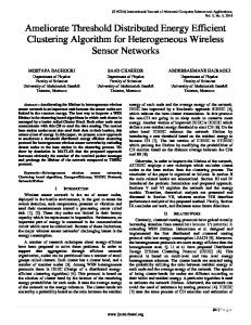
To ensure minimum energy consumption, we will use a very small value for α , which implies that the probability of all sensors being within k hops from at least one volunteer clusterhead is very high. For α = 0.001 and values of p and k computed according to (10) and (12), for a network of 1000 sensors, on an average 1 sensor will not join any volunteer clusterheads and will become a forced clusterhead. The optimal value of p for a network with 1000 nodes in an area of 100 sq. units is 0.08, which means 80 nodes will become volunteer clusterheads on an average. Hence, for a network of 1000 nodes in an area of 100 sq. units, only 1.23 % of all clusterheads are forced clusterheads. C. Simulation Experiments and Results We simulated the algorithm described in Section III for networks with varying sensor density ( d ) and different values of the parameters p and k . In all these experiments, the communication range of each sensor was assumed to be 1 unit. Fig. 1 shows the output of one of these simulations of our algorithm with parameters p and k set to 0.1 and 2 on a network of 500 sensors distributed uniformly in a square area of 100 square units. To verify that the optimal values of the parameters p and k of our algorithms computed according to (10) and (12) do minimize the energy spent in the system, we simulated our clustering algorithm on sensor networks with 500, 1000 and 2000 sensors distributed uniformly in a square area of 100 sq. units. Without loss of generality, it is assumed that the cost of transmitting 1 unit of data is 1 unit of energy. The processing center is assumed to be located at the center of the square area. For the first set of simulation experiments, we considered a range of values for the probability ( p ) of becoming a clusterhead in the algorithm proposed in Section III. For each of these probability values, we computed the maximum number of hops ( k ) allowed in a cluster using (12) and used these values for the maximum number of hops allowed in a cluster in the simulations. The results of these simulations are provided in Fig. 2. Each data point in Fig. 2 corresponds to the average energy consumption over 1000 experiments. It is evident from Fig. 2 that the energy spent in the network is indeed minimum at the theoretically optimal values of the parameter p computed using (10) (let us call this optimal value p opt ),
.
0-7803-7753-2/03/$17.00 (C) 2003 IEEE
(11)
which are given in Table I for 500, 1000 and 2000 sensors in the network.
IEEE INFOCOM 2003
4500
Total Energy Spent
4000
n=2000
3500 3000 2500 n=1000
2000 1500
n=500
1000 500 0
0.05
0.1
0.15
0.2
0.25
0.3
0.35
Probability of becoming a clusterhead
0.4
Figure 1. Output of simulation of the single level clustering algorithm
The experiments were conducted for networks of different densities. For each network density we used our algorithm (described in Section III) to cluster the sensors, with the probability of becoming a clusterhead set to the optimal value ( p opt ) calculated using (10) and maximum number of hops
Figure 2. Total Energy Spent vs. probability of becoming a clusterhead in algorithm in Section III. 9000
ENERGY MINIMIZING PARAMETERS FOR THE ALGORITHM
Number of Sensors ( n )
Density ( d )
500 1000 1500 2000 2500 3000
5 10 15 20 25 30
Probability (
popt )
0.1012 0.0792 0.0688 0.0622 0.0576 0.0541
Maximum Number of Hops (k ) 5 4 3 3 3 3
The computed values of p opt and the corresponding values of maximum number of hops ( k ) in a cluster for networks of various densities are provided in Table I. The results of the simulation experiments are provided in Fig. 3. We observe that the proposed algorithm leads to significant energy savings. The savings in energy increases as the density of sensors in the network increases.
0-7803-7753-2/03/$17.00 (C) 2003 IEEE
d=1
7000 6000 d=3 5000 4000
d=2
3000 Our Algorithm
2000 1000
( k ) allowed between any sensor and its clusterhead equal to the value calculated using p opt in (12). TABLE I.
d=4
8000
Total Energy Spent
Most of the clustering algorithms in the literature (LCA [2], LCA2 [8] and the Highest Degree [9, 24] algorithms) have time complexity of O (n) , which makes them less suitable for sensor networks that have large number of sensors. The MaxMin d-Cluster Algorithm [5] has a time-complexity of O (d ) , which may be acceptable for large networks. Hence, we have compared the performance of our proposed algorithm (with optimal parameter values) and the Max-Min d-cluster algorithm (for d = 1,2,3, 4 ) in terms of the energy spent in the system using simulation.
0
5
10
15
20
25
30
Density of Sensors
Figure 3. Comparison of Our Algorithm and the Max-Min D-Cluster Algorithms .
IV.
A NEW, ENERGY-EFFICIENT, HIERARCHICAL CLUSTERING ALGORTHM In Section III, we have allowed only one level of clustering; we now extend the algorithm to allow more than one level of clustering. Assume that there are h levels in the clustering hierarchy with level 1 being the lowest level and level h being the highest. In this clustered environment, the sensors communicate the gathered data to level-1 clusterheads (CHs). The level-1 CHs aggregate this data and communicate the aggregated data or estimates based on the aggregated data to level-2 CHs and so on. Finally, the level-h CHs communicate the aggregated data or estimates based on this aggregated data to the processing center. The cost of communicating the information from the sensors to the processing center is the energy spent by the sensors to communicate the information to level-1 clusterheads (CHs), plus the energy spent by the level-1
IEEE INFOCOM 2003
CHs to communicate the aggregated information to level-2 CHs, …, plus the energy spent by the level-h CHs to communicate the aggregated information to the information processing center. A. Algorithm The algorithm works in a bottom-up fashion. The algorithm first elects the level-1 clusterheads, then level-2 clusterheads, and so on. The level-1 clusterheads are chosen as follows. Each sensor decides to become a level-1 CH with certain probability p1 and advertises itself as a clusterhead to the sensors within its radio range. This advertisement is forwarded to all the sensors within k1 hops of the advertising CH. Each sensor that receives an advertisement joins the cluster of the closest level-1 CH; the remaining sensors become forced level-1 CHs. Level-1 CHs then elect themselves as level-2 CHs with a certain probability p 2 and broadcast their decision of becoming a level-2 CH. This decision is forwarded to all the sensors within k 2 hops. The level-1 CHs that receive the advertisements from level-2 CHs joins the cluster of the closest level-2 CH. All other level-1 CHs become forced level-2 CHs. Clusterheads at level 3, 4, ..., h are chosen in similar fashion, with probabilities p 3 , p 4 ,..., p h respectively, to generate a hierarchy of CHs, in which any level-i CH is also a CH of level (i-1), (i-2),…, 1. B. Optimal parameters for the algorithm The energy required to communicate the data gathered by the sensors to the information processing center through the hierarchy of clusterheads will depend on the probabilities of becoming a clusterhead at each level in the hierarchy and the maximum number of hops allowed between a member of a cluster and its clusterhead. In this section, we obtain optimal values for the parameters of the algorithm described in Section IV-A that would minimize this energy consumption. To do so, we make the same assumptions as in Section IIIB. Since we have assumed that the sensors are points of a homogeneous Poisson process of intensity λ , the number of sensors in a square area of side 2 a is a Poisson random
Ci : the total cost of communicating information from all level-i CHs to the level-(i+1) CHs, and C : the total cost of communicating information from the sensors to the data processing center through the hierarchy of clusterheads generated by the clustering algorithms. In the proposed algorithm, the sensors elect themselves as level-1 CH with probabilities p1 and the level-i CHs elect themselves as level-(i+1) CHs with probability pi +1 , i = 1,2,..., ( h − 1) . Hence, by properties of the Poisson process, level-i CHs, i = 1, 2,..., h are governed by i
homogeneous Poisson processes of intensities, λ1i = λ ∏ p j . j =1
By arguments similar to those in Section III-B.1, the sum of distance of level-(i-1) CHs from a level-i CH, i = 2,3,..., h in a typical level-i cluster or the sum of distance of sensors from a level-1 CH is given by
E[ Li | N = n] =
i −1 (1 − pi )λ ∏ p j j =1
i 2 λ ∏ p j j =1
3/ 2
.
(13)
The expected number of level-(i-1) CHs in a typical level-i cluster is given by
E[ N i | N = n ] =
1 − pi pi
.
(14)
Therefore, the expected number of hops between a level-(i1) CH and its level-i CH in a typical level-i cluster is given by
1 E[ Li | N = n ] r E[ N i | N = n ]
E[ H i | N = n ] =
2
variable (let’s call this N ) with mean λA , where A = 4 a is the area of the square. Let us assume that for a particular realization of the process, there are n sensors in this area. Let us also define: N i : the number of members in a level-i cluster, Li : the sum of distances between the members of a level-i cluster and their level-i CH, H i : the number of hops from a member to its CH in a typical level-i cluster, TCH i : the total number of level-i CHs,
0-7803-7753-2/03/$17.00 (C) 2003 IEEE
1 = . i 2r λ ∏ p j j =1
(15)
The expected number of level-i CHs is given by i
E[TCH i | N = n] = n ∏ p j . j =1
(16)
IEEE INFOCOM 2003
Hence, the expected total cost of communicating information from all the level-(i-1) CHs to their respective level-i CHs, i = 2,..., ( h − 1), h is given by
E[C i −1 | N = n ] = E[TCH i | N = n]E[ N i | N = n]E[ H i | N = n] .
As apparent from Fig. 6 and Fig. 7, the function in (20) has a very complex form with many local minima. Even if the ceiling of an expression is approximated by just the expression in (20), closed-form solutions for probabilities p i , i = 1,2,..., h that minimize the resulting cost of communication E[C ] have not been obtained, but can be found numerically. Once the optimal probabilities are obtained, following the same arguments as in section III-B.2, k i , i = 1,2,..., h can be calculated according to the equation,
(17)
The expected value of the total cost of communicating information from all the sensors to their level-1 CHs is given by
E[C 0 | N = n ] = E[TCH 1 | N = n ] E[ N 1 | N = n] E[ H 1 | N = n] . (18)
Hence, the expected total cost of communicating information from sensors to the processing center in the clustered environment is given by: E[C | N = n ] h 0.765a h−1 = n ∏ pi + ∑ E [C i | N = n ] i =1 r i =0
i =1
0.765a r
i −1 h 1 + n ∑ (1 − pi ) ∏ ( p j ) . i i =1 j =1 2r λ ∏ p j j =1
(21)
In the above equation, α denotes the probability that the number of hops between a member and the clusterhead in a level-i cluster is more than k i , i = 1, 2,..., h . C. Numerical Results and Simulations We simulated the algorithm described in Section IV-A on networks of sensors distributed uniformly with various spatial densities. In all cases, we assumed that 1 unit of energy spent in communicating 1 unit of data. We use the algorithm to generate a clustering hierarchy with different number of levels in it to see how the energy spent in the network reduces with the increase in number of levels of clusters. In these simulations, we have used the numerically computed set of optimal probabilities (that minimizes E[C ] given by (20)) of becoming clusterheads at each level in the clustering hierarchy. Fig. 4. and Fig. 5 show how the energy consumption decreases as the number of levels in the hierarchy increases. 13.5 n = 25,000 Area = 5,000 sq. units
13
(19)
By un-conditioning on N , we find:
Log (Total Energy Spent)
h
= n ∏ pi
1 − 0.917 ln(α / 7 ) ki = . i r λ∏ p j j =1
12.5 12 11.5
e
E[C ] = E[ E[C | N = n ]] h
= λA∏ p i i =1
0.765a r
10.5 10 0
i −1 h 1 + λA ∑ (1 − p i ) ∏ ( p j ) . i i =1 j =1 2r λ ∏ p j j =1 (20)
0-7803-7753-2/03/$17.00 (C) 2003 IEEE
11
r=1 r=2 r=4
1 2 3 4 Number of levels in the clustering hierarchy
5
Figure 4. Total Energy Spent vs. number of levels in the clustering hierarchy in a network of 25000 sensors with communication radii r distributed in a square area of 5000 sq. units.
IEEE INFOCOM 2003
Hence, they may run out of their energy faster than other sensors. As proposed in [6], the clustering algorithm can be run periodically for load balancing. Instead of running the algorithm periodically, another possibility is that clusterheads trigger the clustering algorithm when their energy levels fall below a certain threshold. Among many other issues, the behavior of the proposed clustering algorithm and the hierarchy generated by it in event of sensor failures is worth investigating.
13.5 n = 25,000 r = 2 units
Log (Total Energy Spent)
13 12.5 12 11.5
e
11
VI.
λ =1.5 λ =5
10.5
λ =10
10 0
1 2 3 4 Number of levels in the clustering hierarchy
5
Figure 5. Total Energy Spent vs. number of levels in the clustering hierarchy in a network of 25000 sensors of communication radius 2 distributed with spatial density λ.
In Fig. 4, we observe that the energy savings are higher for networks of sensors with lower communication radius. These results can be explained as follows. In networks of sensors with higher communication radius, the distance between a sensor and the processing center in terms of number of hops is smaller than the distance in networks of sensors with lower communication radius and hence there is lesser scope of energy savings. The energy savings with increase in the number of levels in the hierarchy are also observed to be more significant for lower density networks. This can be attributed to the fact that among networks of same number of sensors, the networks with lower density has the sensors distributed over a larger area. Hence, in a lower density network, the average distance between a sensor and the processing center is larger as compared to the distance in a higher density network. This means that there is more scope of reducing the distance traveled by the data from any sensor in a non-clustered network, thereby reducing the overall energy consumption.
CONCLUSIONS AND FUTURE WORK
We have proposed a distributed algorithm for organizing sensors into a hierarchy of clusters with an objective of minimizing the total energy spent in the system to communicate the information gathered by these sensors to the information-processing center. We have found the optimal parameter values for these algorithms that minimize the energy spent in the network. In a contention-free environment, the algorithm has a time complexity of O ( k1 + k 2 + ... + k h ) , a significant improvement over the many O (n ) clustering algorithms in the literature [2,3,4,8,9]. This makes the new algorithm suitable for networks of large number of nodes. In this paper, we have assumed that the communication environment is contention and error free; in future we intend to consider an underlying medium access protocol and investigate how that would affect the optimal probabilities of becoming a clusterhead and the run-time of the algorithm.
Since data from each sensor has to travel at least one hop, the minimum possible energy consumption in a network with n sensors is n , assuming each sensor transmits 1 unit of data and the cost of doing so is 1 unit of energy. From Fig. 4 and Fig. 5, it is apparent that the energy consumption is very close to this value when the number of levels in the hierarchy is 5, irrespective of the density of sensors and their communication radius. Hence, if one chooses to store the numerically computed values of optimal probability in the sensor memory, only a small amount of memory would be needed. V.
ADDITIONAL CONSIDERATIONS
The sensors which become the clusterhead in the proposed architecture spend relatively more energy than other sensors because they have to receive information from all the sensors within their cluster, aggregate this information and then communicate to the higher level clusterheads or the information processing center.
0-7803-7753-2/03/$17.00 (C) 2003 IEEE
IEEE INFOCOM 2003
Figure 6. Plot of the energy function in (20) when there are two levels of clusterheads in a network of 10000 sensors of communication range of 4 units distributed in an area of 2500 sq. units.
Figure 7. Contour plot of the energy function in (20) when there are two levels of clusterheads in a network of 10000 sensors of communication range of 4 units distributed in an area of 2500 sq. units.
0-7803-7753-2/03/$17.00 (C) 2003 IEEE
IEEE INFOCOM 2003
REFERENCES [1] [2]
[3] [4]
[5]
[6]
[7]
[8]
[9] [10]
[11]
[12]
[13]
[14]
[15]
[16]
G. J. Pottie and W. J. Kaiser, “Wireless Integrated Network Sensors”, Communications of the ACM, Vol. 43, No. 5, pp 51-58, May 2000. D. J. Baker and A. Ephremides, “The Architectural Organization of a Mobile Radio Network via a Distributed Algorithm”, IEEE Transactions on Communications, Vol. 29, No. 11, pp. 1694-1701, November 1981. B. Das and V. Bharghavan, “Routing in Ad-Hoc Networks Using Minimum Connected Dominating Sets”, in Proceedings of ICC, 1997. C. R. Lin and M. Gerla, “Adaptive Clustering for Mobile Wireless Networks”, Journal on Selected Areas in Communication, Vol. 15 pp. 1265-1275, September 1997. A. D. Amis, R. Prakash, T. H. P. Vuong and D. T. Huynh, “ Max-Min D-Cluster Formation in Wireless Ad Hoc Networks”, in Proceedings of IEEE INFOCOM, March 2000. W. R. Heinzelman, A. Chandrakasan and H. Balakrishnan, “EnergyEfficient Communication Protocol for Wireless Microsensor Networks”, in Proceedings of IEEE HICSS, January 2000. C.F. Chiasserini, I. Chlamtac, P. Monti and A. Nucci, “Energy Efficient design of Wireless Ad Hoc Networks”, in Proceedings of European Wireless, February 2002. A. Ephremides, J.E. Wieselthier and D. J. Baker, “A Design concept for Reliable Mobile Radio Networks with Frequency Hopping Signaling”, Proceeding of IEEE, Vol. 75, No. 1, pp. 56-73, 1987. A. K. Parekh, “Selecting Routers in Ad-Hoc Wireless Networks”, in Proceedings of ITS, 1994. A. Okabe, B. Boots, K. Sugihara and S. N. Chiu, Spatial Tessellations: Concepts and Applications of Voronoi Diagrams, 2nd edition, John Wiley and Sons Ltd. S.G.Foss and S.A. Zuyev, “On a Voronoi Aggregative Process Related to a Bivariate Poisson Process”, Advances in Applied Probability, Vol. 28, no. 4, pp. 965-981,1996. J. M. Kahn, R. H. Katz and K. S. J. Pister, “Next Century Challenges: Mobile Networking for Smart Dust”, in the Proceedings of 5th Annual ACM/IEEE International Conference on Mobile Computing and Networking (MobiCom 99), Aug. 1999, pp. 271-278. F. Baccelli and S. Zuyev, “Poisson Voronoi Spanning Trees with Applications to the Optimization of Communication Networks”, Operations Research, vol. 47, no. 4, pp. 619-631, 1999. B. Warneke, M. Last, B. Liebowitz, Kristofer and S. J. Pister, “Smart Dust: Communicating with a Cubic-Millimeter Computer”, Computer Magazine, Vol. 34, No. 1, pp 44-51, Jan. 2001. J. M. Kahn, R. H. Katz and K. S. J. Pister, “Next Century Challenges: Mobile Networking for Smart Dust”, in the 5th Annual ACM/IEEE International Conference on Mobile Computing and Networking (MobiCom 99), Aug. 1999, pp. 271-278. V. Hsu, J. M. Kahn, and K. S. J. Pister, "Wireless Communications for Smart Dust", Electronics Research Laboratory Technical Memorandum M98/2, Feb. 1998.
0-7803-7753-2/03/$17.00 (C) 2003 IEEE
[17] http://www.janet.ucla.edu/WINS/wins_intro.htm. [18] P. Gupta and P. R. Kumar, “The Capacity of Wireless Networks,”, IEEE Transactions on Information Theory, vol. IT-46, no. 2, pp. 388404, March 2000. [19] P. Gupta and P. R. Kumar, “Critical Power for Asymptotic Connectivity in Wireless Networks”, pp. 547-566, in Stochastic Analysis, Control, Optimization and Applications: A Volume in Honor of W.H. Fleming. Edited by W.M. McEneany, G. Yin, and Q. Zhang, Birkhauser, Boston, 1998. ISBN 0-8176-4078-9. [20] W. Ye, J. Heidemann, and D. Estrin, “An Energy-Efficient MAC Protocol for Wireless Sensor Networks”, In Proceedings of the 21st International Annual Joint Conference of the IEEE Computer and Communications Societies (INFOCOM 2002), New York, NY, USA, June, 2002. [21] N. Bulusu, D. Estrin, L. Girod, and J. Heidemann, “Scalable Coordination for Wireless Sensor Networks: Self-Configuring Localization Systems”, In Proceedings of the Sixth International Symposium on Communication Theory and Applications (ISCTA 2001), Ambleside, Lake District, UK, July 2001. [22] N. Bulusu, J. Heidemann, and D. Estrin, “Adaptive beacon Placement”, Proceedings of the Twenty First International Conference on Distributed Computing Systems (ICDCS-21), Phoenix, Arizona, April 2001. [23] A. B. McDonald, and T. Znati, “A Mobility Based Framework for Adaptive Clustering in Wireless Ad-Hoc Networks”, IEEE Journal on Selected Areas in Communications, Vol. 17, No. 8, pp. 1466-1487, Aug. 1999. [24] M. Gerla, and J. T. C. Tsai, “Multicluster, Mobile, Multimedia Radio Networks”, Wireless Networks, Vol. 1, No. 3, pp. 255-265, 1995. [25] S. Basagni, “Distributed Clustering for Ad Hoc Networks”, in Proceedings of International Symposium on Parallel Architectures, Algorithms and Networks, pp. 310-315, June 1999. [26] S. Basagni, “Distributed and Mobility-Adaptive Clustering for Multinedia Support in Multi-Hop Wireless Networks”, in Proceedings of Vehicular Technology Conference, Vol. 2, pp. 889-893, 1999. [27] M. Chatterjee, S. K. Das, and D. Turgut, “WCA: A Weighted Clustering Algorithm for Mobile Ad hoc Networks”, Journal of Cluster Computing, Special issue on Mobile Ad hoc Networking, No. 5, 2002, pp. 193-204. [28] A.D. Amis, and R. Prakash, “Load-Balancing Clusters in Wireless Ad Hoc Networks”, in Proceedings of ASSET 2000 , Richardson, Texas, March 2000. [29] A. Perrig, R. Szewczyk, V. Wen and J. D. Tygar, “SPINS: Security protocols for Sensor Networks”, in 7th Annual International Conference on Mobile computing and Networking, 2001, pp. 189199. [30] D. W. Carman, P. S. Kruus, and B. J. Matt, “Constraints and approaches for distributed sensor network security”, NAI Labs Technical Report 00-010, September 2000.
IEEE INFOCOM 2003