1
An Evolving Gene Regulatory Network based Spiking Neural Network for Online Human Behavior Recognition Yan Meng, Yaochu Jin, Jun Yin, and Matthew Conforth
Abstract— Automatically understanding human behaviors online in a video stream under various scenes is a challenging task. The major difficulty of this task lies in how to combine the spatial and temporal features of video sequences together to extract behavior patterns. To tackle this problem, we propose an evolving gene regulatory network (GRN) based BCM (E-GRNBCM) model, which is a spiking neural network combined with biological cellular phenomenon. Basically, the weight, weight plasticity, and meta-plasticity of the spiking neural network will be regulated by the GRN, and the GRN will also be influenced by the activity of the neurons it resides in, in a closed loop. Furthermore, an efficient evolutionary algorithm, the covariance matrix adaptation evolution strategy (CMA-ES), is used to justify the GRN parameters, which can significantly reduce the computational cost compared to traditional genetic algorithms. Extensive experimental results have demonstrated the efficiency and robustness of the proposed E-GRN-BCM model for online human behavior recognition under various scenes. Index Terms— Spiking Neural Network, BCM model, Synaptic plasticity and meta-plasticity, Gene regulatory network, covariance matrix adaptation evolution strategy, online human behavior recognition.
I. INTRODUCTION Automatically recognizing human behaviors online in a video stream under various complex scenes is a challenging task for intelligent robots and video surveillance applications due to its large amount of video data to be analyzed and its real-time requirements. Traditionally, most activity recognition work has focused on representing and learning the sequential and temporal characteristics in activity sequences. This has led to the widespread use of dynamic models such as the hidden Markov model (HMM) [1][2][3]. While the HMM is a simple and efficient model for learning sequential data, its performance tends to degrade when the range of activities becomes more complex, or the activities exhibit long-term temporal dependency that is difficult to deal with under the Markov assumption. On the other side, neural network has played a key role for intelligent and cognitive systems. The artificial neuron has a long history, dating back at least to the Threshold Logic Unit in 1943[4]. The artificial neuron is based on a simplistic
Yan Meng, Jun Yin, and Matthew Conforth are with Department of Electrical and Computer Engineering, Stevens Institute of Technology, Hoboken, NJ 07670, USA (Phone: 201-2165496, e-mail:
[email protected],
[email protected] and
[email protected]). Yaochu Jin is with Honda Research Institute Europe, Carl-Legien-Str. 30, 63073, Offenbach, Germany(e-mail:
[email protected]).
abstraction of what a real biological neuron does. Typically it is a node which computes a weighted sum of its inputs and passes the result through a transfer function. This simple model has proved very useful in a variety of connectionist computing and nonlinear modeling tasks. However, we question whether removing the details of biological neurons from artificial neuron has also removed some important neuron behaviors or capabilities. The scientific understanding of biological neurons and neural networks has advanced considerably in the time since artificial neural networks were originally devised. The Bienenstock, Cooper, and Munro (BCM) model [5] is one of the most famous and well-supported modern models of biological neurons [6][7][8]. The BCM model is, more precisely, a model of the plasticity and meta-plasticity of synapses in biological neural networks. Detailed simulations of BCM neurons can provide biologically sound predictions. Edelman et al. [9] used a single layer network and a learning rule based on BCM to extract a visual code in an unsupervised manner. The role of calcium concentration in the spike time dependent plasticity (STDP) of BCM model neurons was investigated by Kurashige and Sakai [10]. Shouval et al. [11] demonstrated evidence for the calcium control hypothesis by comparing biologically motivated models of synaptic plasticity. A reinforcement learning STDP rule developed by Baras and Meir was shown to exhibit statistically similar behavior to the BCM model [12]. While neuroscience has made important progress in modeling the brain, neuro-inspired engineering models are still primarily using simple weighted sum and transform models for artificial neural networks. Detailed biologically accurate neural models are too computationally expensive to replace the simple models for most engineering applications. We intend to develop a compromise model that retains more powerful learning and remembering capability, while sacrificing biological accuracy for better computational efficiency. In this paper, we aim to adapt the BCM model into a computer engineering tool. Since the behavior of a BCM neuron is governed by the local neural activation history, we need another learning mechanism by which to optimize a BCM neural network to a particular task, especially for those tasks that need to extract the temporal features from the input data, such as behavior pattern recognition. To this end, we turn our attention to gene regulatory networks. During the biological morphogenesis, genes in each cell are expressed, resulting in various cellular functions. The expression of the genes is regulated by their own protein
2 products as well as proteins produced by other genes in the same cell or neighboring cells through intracellular and intercellular diffusion, forming a gene regulatory network that can be described by a set of coupled ordinary differential equations. A GRN models the collection of DNA segments in a cell and their indirect interactions with each other via their RNA and protein expression products. GRN models also include some other chemical concentrations in and around the cell which are deemed relevant in their particular context. GRNs play a central role in understanding natural evolution and organism development [13]. Therefore, it is natural for us to use GRN to optimize the BCM model for specific tasks. Therefore, in this paper, we propose an evolving gene regulatory network based BCM (E-GRN-BCM) model, which is a spiking neural network combined with the biological cellular phenomena, and then apply this model to online human behavior recognition. The basic idea of this E-GRN-BCM model is as follows. The BCM based spiking neural network is a graph with weighted, directed edges replacing synapses (since the model need not exist physically in 3D space, dendrites and axons are not necessary). The weight, weight plasticity, and metaplasticity of the spiking neural network will all be regulated by the GRN, and the GRN will be influenced by the activity of the neurons it resides in, in a closed loop. Furthermore, an efficient evolutionary algorithm, i.e., the covariance matrix adaptation evolution strategy (CMA-ES) [19][20], is used to evolve the GRN parameters to optimize the BCM neural network for a specific task, such as online human behavior recognition in a video stream. The neurons will have a spiking rather than continuous output behavior, and each neuron will maintain a recent history for the inclusion of heavily abstracted effects such as spike timing dependent plasticity, ion concentration, membrane potential, etc. The rest of the paper is organized as follows. Section II describes some backgrounds such as the BCM model, the GRN model, and CMA evolution strategy. The E-GRN-BCM model is presented in Section III. Section IV discusses how to apply the E-GRN-BCM model into human behavior recognition. The experimental results on human behavior recognition are shown in Section V. The paper is concluded by Section VI.
A. The BCM Spiking Neuron Model For computational efficiency we use a simplified, discretetime version of the BCM model [5]. The equations governing the behavior of synaptic weights are: ,
1
, ∑ ∑
where
B. The Gene Regulatory Network Multi-cellular morphogenesis is under the control of gene regulatory networks. When a gene is expressed, information stored in the genome is transcribed into mRNA and then translated into proteins. Some of these proteins are transcription factors that can regulate the expression of their own or other genes, thus resulting in a complex network of interacting genes termed as a gene regulatory network (GRN). To understand the emergent morphology resulting from the interactions of genes in a regulatory network, reconstruction of gene regulatory pathways using a computational model has become popular in systems biology. A large number of computational models for GRNs have been suggested [14-18]. Among others, ordinary or partial differential equations have widely been used to model regulatory networks. Mjolsness et al. (1991) proposed a GRN model for describing the gene expression data of developmental processes, which can be considered as a generalized reactiondiffusion model in a continuous form with a sigmoid function: ⎡ ng ⎤ dgij = −γ j gij + φ ⎢ ∑ W jl gil + θ j ⎥ + D j ∇ 2 gij , (4) dt ⎢⎣l =1 ⎥⎦ where gij denotes the concentration of j-th gene product (protein) in the i-th cell. The first term on the right-hand side of Eqn. (4) represents the degradation of the protein at a rate of γ j , the second term specifies the production of protein gij , and the last term describes protein diffusion at a rate of D j .
II. BACKGROUNDS
1
the constant learning rate. is the pre-synaptic input of the th synapse. is the post-synaptic output activation level. is the sliding modification threshold. · is the non-linear activation that swings with the sliding threshold , and it can be defined by Eqn. (2). is the time decay constant that is uniform for all synapses. The interpretation of in Eqn. (3) clearly shows the sliding threshold to be a time-weighted average of squared post-synaptic signals within the time interval of , where is the forgetting factor. The neuron spiking behavior is conceptually relatively simple. If the weighted sum of the pre-synaptic activation levels is less than , or if the neuron fired in the previous time step, then the neuron activation level will decrease. Otherwise, the neuron will fire.
denotes the synaptic weight of the -th synapse.
φ is an activation function for the protein production, which is usually defined as a sigmoid function φ ( z ) = 1/(1 + exp( − μ z )) . The interaction between the genes is described with an interaction matrix W jl , the element of which can be either active (a positive value) or repressive (a negative value). θ j
(1)
is a threshold for activation of gene expression. ng is the number of proteins.
(2)
C. The CMA Evolution Strategy The covariance matrix adaption evolution strategy (CMAES) is a stochastic, iterative optimization method belonging to the class of evolutionary algorithm proposed by Hansen and Ostermeier [19][20]. The covariance matrix adaptation (CMA) is a method to update the covariance matrix of the multivariate
(3) is
3 normal mutation distribution in the evolution strategy. New candidate solutions are sampled according to the mutation distribution. In contrast to classical methods, only the ranking between candidate solutions is exploited during learning. Neither derivatives nor even the function values itself are required by the method. Compared to the traditional evolution algorithms, two important principles of the CMA-ES are: (1) the covariance matrix of the distribution is updated such that the likelihood of previously realized successful steps to appear again is increased; (2) two evolution paths are applied to record the two paths of the time evolution of the distribution mean of the strategy, where one path contains significant information of the correlation between consecutive steps and the other path is used to conduct an additional step-size control. The adaptation of covariance matrix can expedite the overall convergence and the step-size control can make fast convergence to an optimum meanwhile can effectively prevents premature convergence. Another obvious advantage of the CMA-ES is that it does not require a tedious parameter tuning for its applications such that its computational cost can be significantly reduced compared to other traditional genetic algorithms, and this is the main reason for us to choose CMA-ES for as the evolutionary algorithm in this paper due to the real-time performance requirement in online human behavior recognition.
applied here to automatically optimize these parameters for the GRN model to each specific application tasks at hand. More specifically, the covariance matrix adaptation evolution strategy (CMA-ES) is applied to expedite the convergence and reduce the computational cost of the overall system. The block diagram of this E-GRN-BCM model is shown in Fig. 1.
(to be added) Fig. 1. The block diagram of the E-GRN-BCM model.
B. The Basic GRN-BCM Neuron Model To apply the GRN model to regulate the parameters of the BCM model, a series discrete-time differential equations are defined in this sub-section. The gene expression levels of three parameters ( , , ) are defined as: 1
1
,
(5)
1
1
,
(6)
1
1
,
(7)
and the protein expression levels for sodium ion and calcium ion concentration ( , ) are defined as:
III. THE E-GRN-BCM MODEL A. The Framework of the E-GRN-BCM Model We use Eqn. (1)-(3) as the BCM model for our spiking neural network. This spiking neural network can be applied to various real-world applications, such as human behavior recognition in a video stream, or intrusion behavior recognition in a cognitive radio network. To facilitate the online learning capability of this BCM-based spiking neural network, we propose to use a gene regulatory network (GRN) to regulate the tunable parameters ( , , ) of the BCM model in Eqn. (1)-(3), which are used as the output to the GRN model. To apply the GRN dynamics to regulate the parameters of the BCM model to describe the multi-cellular phenomenon, we will make the following assumptions. First, we assume that each BCM parameter corresponds to the expression level of one gene. Second, we assume that, through some chain of mechanisms, the concentrations of the relevant proteins can be deduced from the sodium ion and/or calcium ion concentrations. Finally, we assume that the sodium ion ) is proportional to the concentration (represented by input current and the calcium ion concentration (represented ) is proportional to the activation threshold. by Therefore, the inputs of this GRN regulation consist of two concentrations: sodium ion concentration and calcium ion concentration . Since we will use differential equations to represent the GRN model, there are several parameters in the differential equations need to be defined. As we know, it is very tedious to optimize these parameters for each specific application if we do it manually. Therefore, an evolutionary algorithm is
1
1 ,
where ,
,
(8)
1 ,
,
1 ∑
and
(9) and
are decay factors and
,
are coefficients. Functions f (.),
g(.), and h(.) are defined as the following sigmoid functions: ,
1
(10)
,
1
(11)
,
1
(12)
where k1 and k2 are coefficients. In this basic GRN-SNN model, there are several parameters , , , , , , , , , , , and need to be defined. As a general model, this basic GRNSNN model can be applied to various applications, such as behavior pattern recognition in video streams or cognitive radio networks. However, for each specific task, these parameters need to be carefully tuned so that an optimal performance of the corresponding GRN-BCM model can be achieved. However, fine tuning these parameters for optimal
4 performance is very tedious and time consuming if we do it manually and empirically. Therefore, we plan to use an evolutionary algorithm to automatically generate these parameters for this GRN-BCM model. C. Evolving the GRN-BCM Model using the CMA-ES Since there are 12 parameters need to be adjusted for a single neuron in a spiking neural network, for a simple hierarchical spiking neural network, for example, 3 layers with 24x32 neurons in the input layer, it will be are extremely computational expensive using standard evolutionary algorithms for this GRN-BCM model even if we use very small populations, such as 40. Therefore, we employ a relative efficient evolutionary algorithm, namely, covariance matrix adaptation evolution strategy (CMA-ES), to configure the parameters of the GRN model. The main advantages of using the CMA-ES method are the invariance property in adapting an arbitrarily oriented scaling of the search space and its computational efficiency. , and ) and five The five gamma ( , , , alpha (
,
,
,
, and
~
0,
for
1,
,
(13)
where “~” denotes the same distribution on the left and right side. is the -th solution from generation 1, and , is a vector R , which consists of five gamma ( , , , and ), five alpha ( , , , , and ), and two k ( , and ). The mean vector R represents the favorite solution at generation . is the step size which controls the step length at generation . denotes the covariance matrix at generation and 0, is the -th multivariate normal distribution with zero mean and covariance matrix . , To determine the complete iteration step, , and are defined as: (14)
(15)
1 +
∑
:
(16)
:
1 is the learning rate for the step-size control. where 1 is the damping parameter for step-size update. and are the learning rates for the rank-one update and the rankupdate of the covariance matrix, respectively. is the -th positive weight coefficient for recombination. In addition, the , , and can be obtained from functions generation 1) as follows, ∏
(17)
:
1
) in Eqns. (5)-(9), and two
k ( and ) terms in Eqns. (10)-(12) are constant values to be optimized. Based on the CMA-ES [19], offspring are generated from parents, where denotes the population size (sample size) and denotes the parent population size, i.e. the number of selected points ( ). According to the GRNBCM model, candidate solutions are 12-dimensional vectors of real numbers. The quality of candidate solutions is determined by the objective function. Covariance matrix records the important information between consecutive steps. To increase the probability of repeating the previously successful steps, the covariance matrix of the mutation distribution is to be updated. In other words, this procedure defines the direction of search space and results in a fast convergence. The new values of designated parameters are sampled in a normally distributed way, and the basic equation for each solution at different generations 0,1,2, …, is defined as follows:
1
,
2
(18)
1 ∑
where mass and
2
:
(19)
, is the variance effective selection :
⁄
.
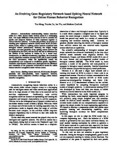
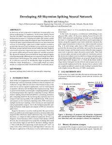
IV. APPLYING THE E-GRN-BCM MODEL TO HUMAN BEHAVIOR RECOGNITION A. The System Framework Now we need to apply the proposed E-GRN-BCM model to online human behavior recognition from video sequences. The system framework of the visual human behavior pattern recognition using the E-GRN-BCM model is shown in Fig. 1. The objective of this system is to online recognize different human behaviors, such as working, running, hand waving, etc., from video sequences automatically. The E-GRN-BCM model takes the full advantage of the spiking neural network (SNN) to implement the human behavior recognition. According to the structure of SNNs, each neuron may have lots of connections with other neurons. For computational efficiency, however, we assume each neuron is only connected to its neighbors and the neural network has three layers, i.e., two middle layers and one top layer. As shown in Fig. 2, the neuron of (1, 1) in the lowermiddle layer is connected to the local neighbor neurons of (1, 2), (2, 1) and (2, 2) within the lower-middle layer. It is noted that only the neurons in the two middle layers can be connected to neighbor neurons of the same layer. In addition, the neuron of (1, 1) has the connections with the neurons of (1,1), (1, 2), (2, 1) and (2, 2) in the upper-middle layer. When the video sequence comes, it will be preprocessed to extract corresponding spatial features frame by frame. Given the features of , each feature is fed into the lower-
5 t middle layer ass an input. Due to the assumption that connnections onlyy exist within local neighborrs, the featuress at thee border havee less connecttions with thee neurons in the low wer-middle layyer than those at the center. To maximaally delliver the inpuut information into the netw work, the low wermiddle layer is designed d with the size of 2 2 . Thhe upper-middlle layer is sett the same sizze with the innput layyer, . The T top layer is the label laayer and is fuully connnected to thee upper-middlee layer, which distinguishes the hum man behavior patterns. p
…... Neurons
… (m,n)
Middle Layeers (1,2)
…...
…
.. ….
…...
.. .
(2 2,2)
…. ..
(1,1) (2,1)
(b)
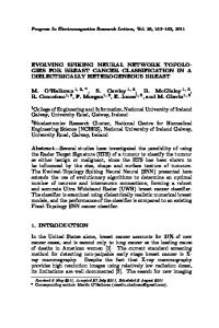
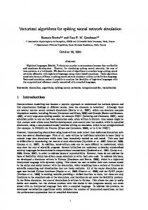
(cc) (d) Fig. 3. 3 An example off extracting the “walking” “ behavvior . ..
.. …. …...
(a)
Label Layerr
…... …
(1,1)
these pooses. Fig. 3 shoows one exampple of extractinng “walking” behavioor features from m a video sequeence.
(m+2,n+2)
…...
Spatial Featurres
…...
Input Frames
Figg. 2. The framew work of the E-G GRN-BCM modeel for visual hum man behhavior recognitioon.
B. Spatial Feaature Extractio B on Generally, eacch video sequeence consists of o a collectionn of varrious frames, which w is the bottom b layer inn this framewoork. Wee adopt 2D innterest point detectors for the detection of spaatial behaviorr features, which w model the geomettric rellationships of the human bo ody. These feaatures of the coocccurrence of moving m pixels represent the low-level vissual feaatures since theey are more relliable in a videoo sequence. One of the most popular approaches to interest pooint dettection in the spatial domain is based onn the detectionn of corrners. Cornerss are defined d as regions where the loocal graadient vectors point in ortho ogonal directioons. The gradiient vecctors are obtaiined by taking the first orderr derivatives of o a , , sm moothed image , , , , where is thee Gaussian sm moothing kernel, and conntrols the spaatial scaale at which coorners are deteected. The respponse strengthh at eacch point is then based on thee rank of the covariance c mattrix of the gradient caalculated in a lo ocal window. F Following thee observation that human behaviors b are the ressults of a seqquence of po oses, a single pattern can be reppresented accoording to the semantic relaationships amoong
C. Suupervised Learrning using thee E-GRN-BCM M Model The extracted spattial behavior features fe are theen fed into a n Since it is a very hierarchhical BCM spiiking neural network. challengging task to exxtract temporaal features from m the image frames directly, the major m advantagee of this hierarrchical BCM mation has beeen naturally model is that the teemporal inform CM model so that the temporal features embeddded into the BC extraction can be skkipped in the preprocessing, which can dramatiically improvee the overall system perfoormance and reduce the t system erroors. Sincce this is a supervised s learrning, during the training process, the GRN model m is used to regulate thhree tunable parametters, i.e., ( , , ), of the BC CM spiking neuural network to learnn specific behavvior patterns ussing example pairs p of input video frrames and outpput labels. The CMA-ES meethod is then applied to automatically generate parameters foor the GRN model. The trained BCM B spiking neural networrk should be able to produce an ouutput that repreesents the behaavior pattern categoryy that currennt input viddeo belongs to. So the architeccture of the neeural network must be consstructed in a layered feed-forward way. w Afteer using this evolving GRN--BCM model for training, the trainned spiking neeural network should not onlly be able to reproduuce the correect output to a given traaining video sequencce, but also bee able to recoggnize the behavvior patterns from thhose unseen innput data if theere is a similarr pattern has been traained before. V. EXPERIMENTALL RESULTS A. Configuration C off Spiking Neurral Network To evvaluate the perrformance of the t proposed E-GRN-SNN E model, several experiiments in diffferent scenarios have been conductted. Basicallyy, the effectiveeness of the framework fr is measureed by two criiteria: how acccurately and robustly the differennt classes of beehavior patternns can be recoognized. We test thhe proposed model usinng the KT TH datasets (http://w www.nada.kth..se/cvap/actionns/) and Weizm mann human motion datasets [21]. For thhese two datasset, the video is usually capptured in the format of o 320 x 240 pixels p per framee. If we use thhe pixel-level input too the spiking neural n network,, the overall coomputational cost woould be very expensive e due the large neurron numbers
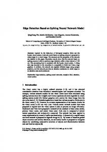
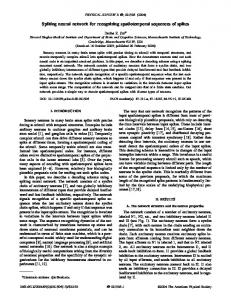
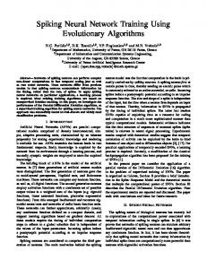
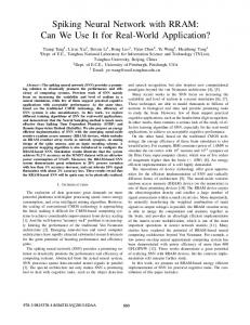
6 t evolutionnary algorithm ms. andd the emplooyment of the Thherefore, as shoown in Fig. 1, in the featuress layer, the inpputs aree reduced to 322x24 in size in proportion to the t original pixxellevvel inputs. Thaat is, the size of o the input layyer in the Fig. 2 is 320 x 240, and the t size of the features layer is 32 x 24. Thhen thee lower-middlee layer is comp posed of 34 x 26 neurons, and a thee upper-middlee layer is comp posed of 32 x 24 neurons. The T labbel layer is fully connected to t the upper-m middle layer. The T CM MA-ES doesn’tt require a larg ge population for f its applicatiion, so here we set 20 and 10. B Behavior Recognition B. R on KTH Dataset The KTH datasset contains seeveral action classes T c perform med by many subjectts. Each video sequence has only one actiion. Figg.4 shows the example of walking, w runniing, hand-waving andd boxing behaviors. We test 400 video seqquences includding theese four behavviors of differeent people. Figg. 5 demonstraates thee extracted spattial features fro om the originall frames. (a)
(a)
(b)
(d) (c) Figg. 4. Example im mages from vid deo sequences inn KTH dataset: (a) waalking behavior, (b) running behavior, (c) handd-waving behavvior, andd (d) boxing behhavior.
The recognitiion rate is defined d as the percentage of ors from the number of all corrrectly recognnized behavio sam mples, which iss N R = R ×100% 1 (18) N whhere R is the recognition raate, N is the number of innput behhaviors, and N R is the nu umber of corrrectly recognizzed behhaviors. Table I shows the recognition results as follows,
Behaviors Walking Running H Hand-waving Boxing Overall
TAB BLE I BEHAVIOR RECOGNITION RESULTS N NR 100 86 100 80 100 87 100 83 400 336
R(%) 86 80 87 83 84
(b)
7 C. Behavior Recognition on Weizmann Dataset Then we evaluate the performance of the E-GRN-BCM model another commonly-used dataset, Weizmann human action dataset [21]. This is a database with 90 low-resolution video sequences showing nine different people, each performing 10 natural actions such as “running,” “walking,” “skipping,” “jumping-jack” (or shortly “jack”), “jumpforward-on-two-legs” (or “jumping”), “jump-in-place- ontwo-legs” (or “pjumping”), “galloping-sideways” (or “siding”), “waving-two-hands” (or “waving2”), “waving-onehand” (or “waving1”), or “bending”. Fig. 6 shows the examples of these behaviors from this database. There are ten different behaviors in total.
(c)
(d) Fig. 5. In the KTH dataset, the original video sequences for behavior patterns of “walking”, “running”, “hand-waving” and “boxing” at top rows, and the extracted spatial features (represented by red shaded areas) from these behavior patterns at the bottom rows. (a) “walking” behavior, (b) “running” behavior, (c) “hand-waving” behavior, (d) “boxing” behavior.
From Table I, it can be seen that the behavior recognition rate on the KTH dataset using the proposed E-GRN-BCM model is high with the overall recognition rate of 84%. That shows that our proposed model turns out to be very effective for human behavior recognition. In a comparison to the previous work of human behavior detection [22][23], our method shows competitive performance as listed in Table II. From Table II, we can see that our proposed E-GRN-BCM model has the highest average recognition rate of 84% compared to other alternative methods. In other words, the proposed E-GRN-BCM model is efficient in supervised learning for online human behavior recognition from video seqences. TABLE II COMPARISON OF DIFFERENT METHODS Methods Recognition Rate Our method 84% Dollar et al. [23] 81.17% Schuldt et al. [22] 71.72%
Learning Labeled Labeled Labeled
(a)
(b)
(c)
(d)
(e)
(f)
(g)
(h)
(i)
(j) Fig. 6. The example images from different behavior video sequences in Weizmann dataset. (a) walking behavior, (b) running behavior, (c) hand-waving behavior, (d) pjumping behavior, (e) siding behavior, (f) jacking behavior, (g) skiping behavior, (h) waving-one-hand behavior, (i) bending behavior, and (j) jumping behavior. TABLE III BEHAVIOR RECOGNITION RESULTS Behaviors Walking Running Hand-waving Pjumping Siding Jacking Skiping Waving1 Bending Jumping Overall
N 9 9 9 9 9 9 9 9 9 9 90
NR 7 6 7 5 7 6 6 7 8 7 66
R (%) 77.78 66.67 77.78 55.56 77.78 66.67 66.67 77.78 88.89 77.78 73.33
From Table III, it can be seen that the recognition results are worse than the previous experiments on KTH dataset. The recognition rates drop a little bit, i.e. from 84% to 73.33%.
8 The reason is that the Weizmann dataset has less human behavior samples, but has more categories of behavior. In addition, some human actions are very close from the motion features. To compare the experimental results with other alternative method, we conduct another set of experiments on the Weizmann dataset using the method proposed in [21]. The comparison results are listed in Table IV. From Table IV, we can see that the performance of our method is much better than the method used in [21]. This result further verified the efficiency of the proposed E-GRN-BCM model for online behavior recognition.
[5]
[6]
[7]
[8]
[9]
[10] TABLE IV COMPARISON OF DIFFERENT METHODS Methods Recognition Rate Our method 73.33% Zelnik et al. [21] 58.91%
Learning Labeled Labeled
[11]
[12] [13]
VI. CONCLUSION AND FUTURE WORK This paper proposed a novel spiking neural network based model for online human behavior recognition, where the gene regulatory networks (GRN) dynamics is used to regulate the plasticity and meta-plasticity of the BCM model and an CMA evolution strategy is applied to automatically generate parameters of GRN dynamics to achieve optimal performance of the BCM model for specific tasks. This so-called E_GRNBCM model takes full advantage of the capabilities of spiking neurons where the processing of temporal data is embedded into the model by their dynamic nature. Furthermore, the evolving GRN-based learning rule is proposed to tackle the intractable problem of tuning the parameters of BCM spiking neural network. Extensive experimental results using two different behavior datasets have demonstrated that the proposed E-GRN-SNN model is very efficient and accurate for online behavior pattern recognition. Although we have made some progress in developing a novel framework for behavior recognition using spiking neural networks, only two different datasets for simple behaviors under structured environments have been tested in this paper to validate the proposed framework. In the future, we will extend this model into a more robust and efficient method for more complex behavior detection and representation in more complex scenes in unstructured environments. REFERENCES [1]
[2]
[3]
[4]
M. T. Chan, A. Hoogs, J. Schmiederer, and M. Perterson. Detecting rare events in video using semantic primitives with HMM. Proc of IEEE International Conference on Pattern Recognition, August 2004. T. Duong, H. Bui, D. Phung, and S. Venkatesh. Activity Recognition and Abnormality Detection with the Switching Hidden Semi-Markov Model. Proc. IEEE Conf. Computer Vision and Pattern Recognition, pp. 838845, 2005. T. Xiang and S. Gong. Video Behavior Profiling for Anomaly Detection. IEEE Trans. on Pattern Analysis and Machine Intelligence, vol. 30, no. 5, 2008, pp. 893-908. McCulloch W. and Pitts, W. A logical calculus of the ideas immanent in nervous activity. Bulletin of Mathematical Biophysics, 7:115 – 133. 1943.
[14]
[15] [16]
[17] [18]
[19] [20]
[21] [22] [23]
Bienenstock, E.L., Cooper, L.N and Munro, P.W. Theory for the development of neuron selectivity: orientation specificity and binocular interaction in visual cortex. The Journal of Neuroscience 2 (1): 32–48. 1982 Dudek, S.M., Bear, M.F. Homosynaptic long-term depression in area CAl of hippocampus and effects of N-methyl-D-aspartate receptor blockade. Proc. Natl. Acad. Sci. USA 89: 4363–4367. May 1992. Kirkwood, A., Rioult, M.G., and Bear, M.F. Experience-dependent modification of synaptic plasticity in visual cortex. Nature 381: 526–528. June 1996. Rittenhouse, C.D., Shouval, H.Z., Paradiso, M.A., and Bear, M.F. Monocular deprivation induces homosynaptic long-term depression in visual cortex. Nature 397: 347-350. Jan 1999. Edelman, S., Intrator, N., and Jacobson, J.S. Unsupervised learning of visual structure. H.H. Bülthoff et al. (Eds.): BMCV 2002, LNCS 2525, pp. 629–642, 2002. Kurashige, H. and Sakai, Y. BCM-type synaptic plasticity model using a linear summation of calcium elevations as a sliding threshold. King et al. (Eds.): ICONIP 2006, Part I, LNCS 4232, pp. 19–29, 2006. Shouval, H.Z., Castellani, G.C., Blais, B.S., Yeung, L.C., Cooper, L.N. Converging evidence for a simplified biophysical model of synaptic plasticity. Springer-Verlag. Biol. Cybern. 87, 383–391. 2002. Baras, D. and Meir, R. Reinforcement learning, spike time dependent plasticity and the BCM rule. Neural Computation 19: 2245–2279. 2007. Alon, U. An Introduction to Systems Biology: Design Principles of Biological Circuits. Chapman & Hall/CRC, July 2006. De Jong, H. Modeling and simulation of genetic regulatory systems: a literature review. Journal of Computational Biology, vol. 9, no. 1, pp. 67-103. 2002. Endy, D. and Brent, R. Modeling cellular behavior. Nature 409, 391395. 2001. Hasty, J., McMillen, D., Isaacs, F., and Collins, J.J. Computational studies of gene regulatory networks: in numero molecular biology. Nat. Rev. Genet. 2, 268-279. 2001. McAdams, H.H. and Arkin, A. Simulation of prokaryotic genetic circuits. Ann. Rev. Biophys. Biomol. Struct. 27, 199-224. 1998. Smolen, P., Baxter, D.A., and Byrne, J.H., Modeling transcriptional control in gene networks: methods, recent results, and future directions. Bull. Math. Biol. 62, 247-292. 2000. Hansen N, Ostermeier A. Completely derandomized self-adaptation in evolution strategies. Evolutionary Computation, 9(2) pp.159-195. 2001. Hansen N, Müller SD, Koumoutsakos P. Reducing the time complexity of the derandomized evolution strategy with covariance matrix adaptation (CMA-ES). Evolutionary Computation, 11(1) pp.1-18. 2003. L. Zelnik-Manor and M. Irani, Event-Based Analysis of Video, ComputerVision and Pattern Recognition, pp. 123-130, Sept. 2001. Christian Schuldt, Ivan Laptev, and Barbara Caputo. Recognizing human actions: A local svm approach. In ICPR, pages 32–36, 2004. Piotr Doll´ar, Vincent Rabaud, Garrison Cottrell, and Serge Belongie. Behavior recognition via sparse spatio-temporal features. In VS-PETS 2005, pages 65–72, 2005.