Dec 14, 2010 - [1] Jiong Guo, Falk Hüffner, Christian Komusiewicz, and Yong Zhang. Improved algorithms for bicluster editing. In TAMC'08: Proceedings of the ...
An Improved Algorithm for Bipartite Correlation Clustering Nir Ailon∗ Noa Avigdor-Elgrabli† Edo Liberty‡
arXiv:1012.3011v1 [cs.DS] 14 Dec 2010
Abstract Bipartite Correlation clustering is the problem of generating a set of disjoint bi-cliques on a set of nodes while minimizing the symmetric difference to a bipartite input graph. The number or size of the output clusters is not constrained in any way. The best known approximation algorithm for this problem gives a factor of 11.1 This result and all previous ones involve solving large linear or semi-definite programs which become prohibitive even for modestly sized tasks. In this paper we present an improved factor 4 approximation algorithm to this problem using a simple combinatorial algorithm which does not require solving large convex programs. The analysis extends a method developed by Ailon, Charikar and Alantha in 2008, where a randomized pivoting algorithm was analyzed for obtaining a 3-approximation algorithm for Correlation Clustering, which is the same problem on graphs (not bipartite). The analysis for Correlation Clustering there required defining events for structures containing 3 vertices and using the probability of these events to produce a feasible solution to a dual of a certain natural LP bounding the optimal cost. It is tempting here to use sets of 4 vertices, which are the smallest structures for which contradictions arise for Bipartite Correlation Clustering. This simple idea, however, appears to be evasive. We show that, by modifying the LP, we can analyze algorithms which take into consideration subgraph structures of unbounded size. We believe our techniques are interesting in their own right, and may be used for other problems as well.
∗
Technion Israel Institute of Technology. Technion Israel Institute of Technology and Yahoo! Research. ‡ Yahoo! Research. 1 A previously claimed 4- approximation algorithm [1] is erroneous, as we show in the appendix. †
1
Introduction
Bipartite Correlation Clustering (BCC) is a problem in which the input is a bipartite graph and the output is a set of disjoint clusters covering the graph nodes.2 A cluster may contain nodes from either side of the graph, but it may also contain nodes from only one side. We think of a cluster as a bi-clique connecting all the elements from its left and right counterparts. An output clustering is hence a union of bi-cliques covering the input node set. The cost of the solution is the symmetric difference between the input and the output. Equivalently, any pair of vertices, one on the left and one of the right, will incur a unit cost if either (1) an edge connects them but the output clustering separates them in distinct clusters, or (2) no edge connects them but the output clustering puts them in the same cluster. The objective is to minimize this cost. This notion of clustering is natural when the number of clusters and their size are not known, and the graph relations are bipartite by nature. It was studied in context of molecular biology, specifically, in gene expression data analysis (for example [2, 3]). Other examples for bipartite data abound. In collaborative filtering and recommender systems interactions are given between users and items [4], for example, raters vs. movies/songs. Other examples may include images vs. user generated tags and search engine queries vs. search results. BCC is a bipartite version of the more well known Correlation Clustering (CC), introduced by Bansal, Blum and Chawla [5], where the objective is to cover an input set of nodes with disjoint cliques (clusters) minimizing the symmetric difference with a given edge set over these nodes. One motivation for BCC, which also applies to our setting, is a 2-stage clustering approach in which one (i) applies binary classification machine-learning methods to predict pairs of nodes that should be clustered together, and (ii) uses the learned classifier, applied to all pairs, as input to BCC. Assuming there is a correct clustering of the data and that the above binary classifier has some bounded error rate with respect to that ground truth, we can recover, using an algorithm for CC (or, BCC in our bipartite case) a clustering of the data which is provably close to the true clustering (see [11]). Another motivation is the alleviation of the need to specify the number of output clusters, as often needed in clustering settings such as k-means or k-median. The treatment of clustering problems as CC or BCC should be compared to their predating (by decades) statistical theory of record linkage where, in a typical application, one wishes to identify duplicate records in a database riddled with human errors. The number of clusters is clearly unknown. In fact, the original record linkage literature [7] considered the bipartite case, a typical example being two government agencies cross-validating large databases of population information. Bansal et. al [5] gave a c ≈ 104 factor for approximating CC running in time O(n2 ) where n is the number of nodes in the graph. Later, Demaine et. al [8] gave a O(log(n)) approximation algorithm for an incomplete version of CC, relying on solving an LP and rounding its solution by employing a region growing procedure. By incomplete we mean that only a subset of the node pairs participate 2
Here we consider the unweighted case, although a weighted version can be easily obtained from our analysis.
1
in the symmetric difference cost calculation.3 BCC is, in fact, a special case of incomplete CC, in which the non-participating node pairs lie on the same side of the graph. Charikar et. al [9] provide a 4-approximation algorithm for CC, and another O(log n)-approximation algorithm for the incomplete case. Later, Ailon et. al [10] provided a 2.5-approximation algorithm for CC based on rounding an LP. They also provide a simpler 3-approximation algorithm, QuickCluster, which runs in time linear in the number of edges of the graph. In [11] it was argued that QuickCluster runs in expected time O(n + cost(OP T )). Van Zuylen et. al [12] provided de-randomization for the algorithms presented in [10] with no compromise in the approximation guarantees. Mathieu and Schudy in [13] considered the planted graph version, in which the input is a noisy version of a union-of-cliques graph, and show that a PTAS is possible for this setting. Also, Giotis et. al [14] and independently using other techniques, Karpinski et. al [15] gave a PTAS for the CC case in which the number of clusters is constant. Amit [16] was the first to address BCC directly. She proved its NP-hardness and gave a constant 11-approximation algorithm based on rounding a linear programming in the spirit of Charikar et. al’s [9] algorithm for CC. It is worth noting that in [1] a 4-approximation algorithm for BCC was presented and analyzed. The presented algorithm is incorrect (we give a counter example in the paper) but their attempt to use arguments from [10] is an excellent one. We will show that an extension of the method in [10] is needed.
1.1
Our Results
Our main result, requiring a considerable development of previous techniques, is a randomized expected 4-approximation algorithm, PivotBiCluster. To explain how we attain it, we recall the method of Ailon et. al [10]. The algorithm for CC presented there is as follows (we concentrate on the unweighted case). Choose a random vertex, and form a cluster with its neighbors. Remove the cluster from the graph, and repeat until the graph is empty. This random-greedy algorithm returns a solution with cost at most 3-times that of the optimal solution, on expectation. The analysis was done by noticing that each cost element is naturally related to a contradiction structure containing 3 vertices and exactly 2 edges between them. This structure is, incidentally, the minimal structure forcing any solution to pay. In other words, the locations in which any clustering errs must hit the set of contradicting structures. A corresponding hitting set LP lower bounding the optimal solution was defined to capture this simple observation, and a feasible solution was then conveniently assigned to its dual using probabilities arising in the algorithm probability space. It is tempting here to consider the corresponding minimal contradiction structure for BCC, namely a set of 4 vertices, 2 on each side, with exactly 3 edges between them. Unfortunately, this idea turned out to be evasive (a proposed solution attempting this [1] has a counter example which we describe and analyze in Appendix A and is hence incorrect). In our analysis we resorted to 3
In some of the literature, CC refers to the much harder incomplete version, and “CC in complete graphs” is used for the version we have described here.
2
contradiction structures of unbounded size. Such a structure consists of two vertices `1 , `2 of the left side and two sets of vertices N1 , N2 on the right hand side such that Ni is contained in the neighborhood of `i for i = 1, 2, N1 ∩ N2 6= ∅ and N1 6= N2 . We define a hitting LP as we did earlier, this time of possibly exponential size, and analyze its dual in tandem with a carefully constructed random-greedy algorithm. As this analysis sketch suggests, the algorithm is not symmetrical with respect to the right and left side of the input. Indeed, at each round it chooses a random pivot vertex on the left, constructs a cluster with its right hand side neighbors, and then for each other vertex on the left hand side makes a randomized decision whether to join the new cluster based on the intersection pattern of its neighborhood with the pivot’s neighborhood.
1.2
Paper Structure
We start with basic notation in Section 2. We then present our main algorithm in Section 3, followed by its analysis in Section 4. We discuss future work in Section 5.
2
Notation
Before describing the framework we give some general facts and notations. Let the input graph be G = (L, R, E) where L and R are the sets of left and right nodes and E be a subset of L × R. Each element (`, r) ∈ L × R will be referred to as a pair. A solution to our combinatorial problem is a clustering C1 , C2 , . . . , Cm of the set L ∪ R. We identify such a clustering with a bipartite graph B = (L, R, EB ) for which (`, r) ∈ EB if and only if ` ∈ L and r ∈ R are in the same cluster Ci for some i. Note that given B, we are unable to identify clusters contained exclusively in L (or R), but this will not affect the cost, so we adopt the convention that single-side clusters are always singletons. We will say that a pair e = (`, r) is erroneous if e ∈ (E \ EB ) ∪ (EB \ E). For convenience, let xG,B be the indicator function for the erroneous pair set, i.e., xG,B (e) = 1 if e is erroneous and 0 otherwise. We will also simply use x(e) when it is obvious to which graph G and clustering B it P refers. The cost of a clustering solution is defined to be costG (B) = e∈L×R xG,B (e). Similarly, P we will use cost(B) = e∈L×R x(e) when G is clear from the context, Let N (`) = {r|(`, r) ∈ E} be the set of all right nodes adjacent to `. It will be convenient for what follows to define a tuple. We define a tuple T to be T = T T , RT ) where `T , `T ∈ L, `T 6= `T , RT ⊆ N (`T ) \ N (`T ), RT ⊆ N (`T ) \ N (`T ) (`1 , `T2 , R1T , R1,2 2 1 2 1 2 1 1 2 2 2 1 T and R1,2 ⊆ N (`T2 ) ∩ N (`T1 ). In what follows, we may omit the superscript of T . Given a T , RT ), we define the conjugate tuple T ¯ = (`T¯ , `T¯ , RT¯ , RT¯ , RT¯ ) = tuple T = (`T1 , `T2 , R1T , R1,2 1,2 2 1 2 1 2 ¯ = T. T , RT ). Note that T (`T2 , `T1 , R2T , R1,2 1
3
joins w.p. 1
becomes a singleton w.p. 1
joins w.p. 2/3
becomes a singleton w.p. 1/2
Figure 1: Four example cases in which `2 either joins the cluster created by `1 or becomes a singleton. In the two right most examples, with the remaining probability nothing is decided about `2 .
3
The Algorithm
We now describe our algorithm PivotBiCluster. The algorithm is sequential. In every cycle it creates one cluster and possibly many singletons, all of which are removed from the graph before continuing to the next iteration. Abusing notation, by N (`) we mean, in the algorithm’s description, all the neighbors of ` ∈ L which have not yet been removed from the graph. Every such cycle performs two phases. In the first phase, PivotBiCluster picks a node on the left side uniformly at random, `1 , and forms a new cluster C = {`1 } ∪ N (`1 ). This will be referred to as the `1 -phase and `1 will be referred to as the left center of the cluster. In the second phase, denoted as the `2 -sub-phase corresponding to the `1 -phase, the algorithm iterates over all other remaining left nodes, `2 , and decides either to (1) append them to C, (2) turn them into singletons, or (3) do nothing. We now explain how to make this decision. let R1 = N (`1 ) \ N (`2 ), R2 = N (`2 ) \ N (`1 ) |R | , 1} do one of two things: (1) If |R1,2 | ≥ |R1 | and R1,2 = N (`1 ) ∩ N (`2 ). With probability min{ |R1,2 2| append `2 to C, and otherwise (2) (if |R1,2 | < |R1 |), turn `2 into a singleton. In the remaining probability, (3) do nothing for `2 , leaving it in the graph for future iterations. Examples for cases the algorithm encounters for different ratios of R1 , R1,2 , and R2 are given in Figure 3. Theorem 3.1. Algorithm PivotBiCluster returns a solution with expected cost at most 4 that of the optimal solution.
4
Algorithm Analysis
We start by describing bad events. This will help us relate the expected cost of the algorithm to a sum of event probabilities and expected consequent costs. T , RT ) if Definition 4.1. We say that a bad event, XT , happens to the tuple T = (`T1 , `T2 , R1T , R1,2 2 during the execution of PivotBiCluster, `T1 was chosen to be a left center while `T2 was still in the T = N (`T )∩N (`T ), and RT = N (`T )\N (`T ). graph, and at that moment, R1T = N (`T1 )\N (`T2 ), R1,2 1 2 2 2 1 (We refer by N (·) here to the neighborhood function in a particular moment of the algorithm execution.)
4
If a bad event XT happens to tuple T we “color” the following pairs with color T : • {(`T2 , r1 ) : r1 ∈ R1T }, T }, • {(`T2 , r1,2 ) : r1,2 ∈ R1,2
• {(`T2 , r2 ) : r2 ∈ R2T } only if we decide to associate `T2 to `T1 ’s cluster, or if we decide to make `T2 a singleton during the `2 -sub-phase corresponding to the `1 -phase. Lemma 4.1. During the execution of PivotBiCluster each pair (`, r) ∈ L × R is colored at most once, and each pair on which the output errs is colored exactly once. Proof. For the first part, we show that pairs are colored at most once. A pair (`, r) can only be colored during an `2 -sub-phases with respect to some `1 -phase, if ` = `2 . Clearly, this will only happen in one `1 -phase, as every time a pair is colored either `2 or r (or both) are removed from the graph. Indeed, either r ∈ R1 ∪ R1,2 in which case r is removed, or r ∈ R2 , but then ` is removed since it either joins the cluster created by `1 or becomes a singleton. For the second part, note that the only pairs which are not colored are between left centers (during `1 -phases) and right nodes in the graph at that time. On all these pairs the algorithm does not err. � We denote by qT the probability that event XT occurs and by cost(T ) the number of erroneous pairs that are colored by XT . From Lemma 4.1 we get the following: Corollary 4.1. "
# X
E[cost[P ivotBiCluster]] = E
"
x(e) = E
e∈L×R
# X T
cost(T ) =
X
qT · E[cost(T )|XT ] .
T
Note: In what follows we use the terms erroneous pairs and violating pairs or violation pairs interchangingly, referring to pairs on which the algorithm incurs a unit of cost.
4.1
Contradicting Structures
We now identify bad structures in the graph for which every output must incur some cost. In the case of BCC the minimal such structures are “bad squares”: A set of four nodes, two on each side, between which there are only three edges. We make the trivial observation that any clustering B must make at least one mistake on any such bad square, s (we think of s as the set of 4 pairs connecting its two left nodes and two right nodes). Any clustering solution’s violating pair set must hit these squares. Let S denote the set of all bad squares in the input graph G. It is not enough to concentrate on squares in our analysis. Indeed, at an `2 -sub-phase, decisions are made based on the intersection pattern of the current neighborhoods of `2 and `1 - a possibly unbounded structure. The tuples now come in handy. T , RT ) for which |RT | > 0 and |RT | > 0 . Notice that Consider tuple T = (`T1 , `T2 , R1T , R1,2 2 1,2 2 T the tuple contains the bad square induced by for every selection of r2 ∈ R2T , and r1,2 ∈ R1,2 5
{`1 , r2 , `2 , r1,2 }. Note that there may also be bad squares {`2 , r1 , `1 , r1,2 } for every r1 ∈ R1T and T but these will be associated to the conjugate tuple T ¯ = (`T , `T , RT , RT , RT ). r1,2 ∈ R1,2 2 1 2 1,2 1 For each tuple we can write a corresponding linear constraint on the function {x(e) : e ∈ L×R}, indicating, as we explained above, the pairs for which the algorithm errs. A tuple constraint is the sum of the constraints of the squares it is associated with, where a constraint for square s is simply P T | bad squares, we get the defined as e∈s x(e) ≥ 1. Since each tuple corresponds to |R2T | · |R1,2 following constraint: � � X ∀T : x`T ,r2 + x`T ,r1,2 + x`T ,r2 + x`T ,r1,2 = 1
1
2
2
T r2 ∈R2T ,r1,2 ∈R1,2
X
T |R1,2 | · (x`T ,r2 + x`T ,r2 ) +
X
T | |R2T | · (x`T ,r1,2 + x`T ,r1,2 ) ≥ |R2T | · |R1,2 2
1
2
1
T r1,2 ∈R1,2
r2 ∈R2T
The following linear program hence provides a lower bound for the optimal solution:
LP
=
X
min
x(e)
e∈L×R
s.t. ∀ T
1 X 1 (x`T ,r2 + x`T ,r2 ) + T T 1 2 |R2 | |R1,2 | T r2 ∈R2
X
(x`T ,r1,2 + x`T ,r1,2 ) ≥ 1 1
2
T r1,2 ∈R1,2
Notice that all the constraints in this program are sums of square constraints. This means that the program is equivalent to one in which only square constraints are present. Our formulation, however, allows the definition of useful dual variables corresponding to each tuple T . The dual program is as follows:
DP
=
max
X
β(T )
T
s.t. ∀ (`, r) ∈ E :
X T T : `T 2 =`,r∈R2
and ∀ (`, r) 6∈ E :
X T T : `T 1 =`, r∈R2
4.2
X 1 β(T ) + |R2T | T
T T : `1 =`, r∈R1,2
X 1 β(T ) + T | |R1,2 T
T T : `2 =`, r∈R1,2
1 β(T ) ≤ 1 T | |R1,2
1 β(T ) ≤ 1 |R2T |
Obtaining the Competitive Analysis
We now relate the expected cost of the algorithm on each tuple to a feasible solution for DP . We remind the reader that qT denotes the probability that a bad event XT happens to tuple T . T |, |RT |} , when Lemma 4.2. Let β(T ) = αT · qT · min{|R1,2 2
6
( αT = min 1,
)
T | |R1,2 T |, |RT |} + min{|RT |, |RT |} min{|R1,2 2 1,2 1
then β is a feasible solution to DP . In other words, for every edge e = (`, r) ∈ E: X T s.t
T `T 2 =`,r∈R2
1 β(T ) + |R2T |
X T s.t
T `T 1 =`, r∈R1,2
1 β(T ) + T | |R1,2
X T s.t
T `T 2 =`, r∈R1,2
1 β(T ) ≤ 1. T | |R1,2
(1)
And for every pair e = (`, r) 6∈ E: 1 β(T ) ≤ 1 . |R2T |
X T s.t
T `T 1 =`, r∈R2
(2)
Proof. First, notice that given a pair e = (`, r) ∈ E each tuple T can appear at most in one of the sums in the LHS of (1). Denote by Xe,T the event that the edge e is colored with color T . We distinguish between two cases. 1. Consider T appearing in the first sum of the LHS of (1), meaning that `T2 = ` and r ∈ R2T . We distinguish between two sub-cases. T | ≥ |RT |, e is colored with color T if `T joined the cluster of `T . This happens, • If |R1,2 1 2 � � 1 T | |R1,2 conditioned on XT , with probability Pr[Xe,T |XT ] = min |RT | , 1 , 2
• if
T | |R1,2
|RT | > |RT |) : Case 2. |R1T | < |R1,2 2 1 1,2 2 � � T | |R1,2 Here αT = αT¯ = min 1, |RT |+|RT | , therefore, 1
1,2
� T T β(T ) + β(T¯) = αT · qT · min{|R1,2 |, |R2T |} + min{|R1,2 |, |R1T |} T T T = qT · min{|R1,2 | + |R1T |, |R1,2 |} = qT · |R1,2 |. T |, if event X happens PivotBiCluster adds `T to `T cluster with probability As |R1T | ≤ |R1,2 T 2 1 � � T | T | T | |R1,2 |R1,2 |R1,2 min |RT | , 1 = |RT | . Therefore with probability |RT | the pairs colored by color T that Pivot2
2
2
`T2
BiCluster violate are all to and all the non-edges from `T2 to R1T , and with � � the edges from |R | T . Thus, probability 1 − |R1,2 PivotBiCluster violates all the edges from `T2 to R1,2 2| E[cost(T )|XT ] =
T | |R1,2
|R2T |
R2T
� |R2T | + |R1T | +
T = 2 · |R1,2 |+
1−
T | |R1,2
|R2T |
T | · |RT | − |RT |2 |R1,2 1 1,2
|R2T |
9
! T |R1,2 |
T |. ≤ 2 · |R1,2
¯
¯
T | and min If the event XT¯ happens, as |R1T | > |R1,2
�
�
¯
T R1,2 ¯
R2T
,1
= 1, PivotBiCluster chooses to isolate
¯ `T2 (= `T1 ) with probability 1 and the number of pairs colored with color T¯ that are consequently ¯ T¯ | = |RT | + |RT | . Thus, violated are |R2T | + |R1,2 1 1,2
� T T qT · E[cost(T )|XT ]) + E[cost(T¯)|XT¯ )] ≤ qT · (2|R1,2 | + |R1T | + |R1,2 |) � T < 4 · qT · |R1,2 | = 4 · β(T ) + β(T¯) . ¯
¯
¯
¯
T | < |RT |, |RT | < |RT | (equivalently, |RT | < |RT |, |RT | < |RT |): Case 3. |R1,2 1 1,2 2 1,2 1 1,2 2 Here, αT = αT¯ = 12 , thus,
� 1 T T T β(T ) + β(T¯) = · qT · min{|R1,2 |, |R2T |} + min{|R1,2 |, |R1T |} = qT · |R1,2 |. 2 T |, PivotBiCluster chooses to isolate ` with probability Conditioned on event XT , as |R1T | > |R1,2 2 � � T T T | |R1,2 | |R1,2 | |R1,2 T | pairs min |RT | , 1 = |RT | . Therefore with probability |RT | PivotBiCluster colors |R2T | + |R1,2 2 2 2 � � T | |R1,2 T | with color T (and violated them all). With probability 1 − |RT | , PivotBiCluster colors |R1,2 2
pairs with color T (and violated them all). We conclude that E[cost(T )|Xt ] =
Similarly, for event XT¯ , as with probability
T | |R1,2 |R1T |
With probability (1 − Thus,
T | |R1,2
|R2T |
¯ |R1T |
>
(|R2T |
T¯ | |R1,2
+
T |R1,2 |)
1−
+ �
and min
¯
T | |R1,2 ¯ |R2T |
T | |R1,2
! T T |R1,2 | = 2|R1,2 |.
|R2T |
� ,1 =
T | |R1,2 , |R1T |
PivotBiCluster isolates `1
¯ T¯ | pairs with color T ¯ (and violated them all). therefore colors |R2T | + |R1,2 T | |R1,2 ) |R1T |
T¯ | pairs with color T ¯ (and violates them all). PivotBiCluster colors |R1,2
E[cost(T¯)|XT¯ ] =
T | |R1,2
|R1T |
(|R1T |
+
T |R1,2 |)
+
1−
T | |R1,2
|R1T |
! T T |R1,2 | = 2|R1,2 |.
And therefore � T qT · E[cost(T )|Xt ] + E[cost(T¯)|XT¯ ] = 4 · qT · |R1,2 | = 4 · (β(T ) + β(T¯)) . � By Corollary 4.1 E[P ivotBiCluster] =
X
Pr[XT ] · E[cost(T )|XT ]
T
=
� 1X Pr[XT ] · E[cost(T )|XT ] + Pr[XT¯ ] · E[cost(T¯)|XT¯ ] . 2 T
10
By Lemma 4.3 the above RHS is at most 2 · weak duality theorem we conclude that
P
T (β(T )
E[P ivotBiCluster] ≤ 4 ·
X
+ β(T¯)) = 4 ·
P
T
β(T ). Therefore by the
β(T ) ≤ 4 · OP T.
T
This proves our main result Theorem 3.1.
5
Future Work
Improving the approximation factor as well as derandomizing the algorithm (in the lines of [12], or using other techniques) are interesting questions. One direction that seems promising is to devise an LP rounding algorithm using a variation of PivotBiCluster (in the lines of the LP-based algorithms in [10]).
References [1] Jiong Guo, Falk H¨ uffner, Christian Komusiewicz, and Yong Zhang. Improved algorithms for bicluster editing. In TAMC’08: Proceedings of the 5th international conference on Theory and applications of models of computation, pages 445–456, Berlin, Heidelberg, 2008. SpringerVerlag. [2] Sara C. Madeira and Arlindo L. Oliveira. Biclustering algorithms for biological data analysis: A survey. IEEE/ACM Trans. Comput. Biol. Bioinformatics, 1:24–45, January 2004. [3] Yizong Cheng and George M. Church. Biclustering of expression data. In Proceedings of the Eighth International Conference on Intelligent Systems for Molecular Biology, pages 93–103. AAAI Press, 2000. [4] Panagiotis Symeonidis, Alexandros Nanopoulos, Apostolos Papadopoulos, and Yannis Manolopoulos. Nearest-biclusters collaborative filtering, 2006. [5] Nikhil Bansal, Avrim Blum, and Shuchi Chawla. Correlation clustering. Machine Learning, 56:89–113, 2004. 10.1023/B:MACH.0000033116.57574.95. [6] Bianca Zadrozny, John Langford, and Naoki Abe. Cost-sensitive learning by cost-proportionate example weighting, 2003. [7] Ivan P. Fellegi and Alan B. Sunter. A theory for record linkage. Journal of the American Statistical Association, 64(328):1183–1210, 1969. [8] Erik D. Demaine, Dotan Emanuel, Amos Fiat, and Nicole Immorlica. Correlation clustering in general weighted graphs. Theoretical Computer Science, 2006.
11
[9] Moses Charikar, Venkatesan Guruswami, and Anthony Wirth. Clustering with qualitative information. J. Comput. Syst. Sci., 71(3):360–383, 2005. [10] Nir Ailon, Moses Charikar, and Alantha Newman. Aggregating inconsistent information: Ranking and clustering. J. ACM, 55(5):1–27, 2008. [11] Nir Ailon and Edo Liberty. Correlation clustering revisited: The ”true” cost of error minimization problems. In ICALP ’09: Proceedings of the 36th International Colloquium on Automata, Languages and Programming, pages 24–36, Berlin, Heidelberg, 2009. Springer-Verlag. [12] Anke van Zuylen, Rajneesh Hegde, Kamal Jain, and David P. Williamson. Deterministic pivoting algorithms for constrained ranking and clustering problems. In SODA ’07: Proceedings of the eighteenth annual ACM-SIAM symposium on Discrete algorithms, pages 405–414, Philadelphia, PA, USA, 2007. Society for Industrial and Applied Mathematics. [13] Claire Mathieu and Warren Schudy. Correlation clustering with noisy input. In SODA, pages 712–728, 2010. [14] Ioannis Giotis and Venkatesan Guruswami. Correlation clustering with a fixed number of clusters. In Proceedings of the seventeenth annual ACM-SIAM symposium on Discrete algorithm, pages 1167–1176, 2006. [15] Marek Karpinski and Warren Schudy. Linear time approximation schemes for the galeberlekamp game and related minimization problems. CoRR, abs/0811.3244, 2008. [16] Noga Amit. The bicluster graph editing problem. Master Thesis, 2004.
A
A Counter Example for a Previously Claimed Result
In [1] the authors claim to design and analyze a 4-approximation algorithm for BCC. Its analysis is based on bad squares (and not unbounded structures, as done in our analysis). Their algorithm is as follows: First, choose a pivot node uniformly at randomly from the left side, and cluster it with all its neighbors. Then, for each node on the left, if it has a neighbor in the newly created cluster, append it with probability 1/2. An exception is reserved for nodes whose neighbor list is identical that of the pivot, in which case these nodes join with probability 1. Remove the clustered nodes and repeat until no nodes are left in the graph. Unfortunately, there is an example demonstrating that the algorithm has an unbounded approximation ratio. Consider a bipartite graph on 2n nodes, `1,...,n on the left and r1,...,n on the right. Let each node `i on the left be connected to all other nodes on the right except for ri . The optimal clustering of this graph connects all `i and ri nodes and thus has cost OP T = n. In the above algorithm, however, the first cluster created will include all but one of the nodes on the right and roughly half the left ones. This already incurs a cost of Ω(n2 ) which is a factor n worse than the best possible. 12
As a side note, the authors of this abstract have also tried to design an algorithm based on an analysis involving squares only, to no avail.
13