Abstract. Neural networks have played an important role in intelligent medical diagnoses. This paper presents an Improved Constructive Neural. Network ...
An Improved Constructive Neural Network Ensemble Approach to Medical Diagnoses Zhenyu Wang, Xin Yao, and Yong Xu CERCIA, School of Computer Science, The University of Birmingham, Birmingham B15 2TT, UK {msc44zxw, x.yao, y.xu}@cs.bham.ac.uk Abstract. Neural networks have played an important role in intelligent medical diagnoses. This paper presents an Improved Constructive Neural Network Ensemble (ICNNE) approach to three medical diagnosis problems. New initial structure of the ensemble, new freezing criterion, and a different error function are presented. Experiment results show that our ICNNE approach performed better for most problems.
1
Introduction
Recently, using artificial neural network (NN) for medical purposes has been shown to be an interesting topic. Most of the work has been focused on achieving better classification performance. A NN ensemble (NNE) consisting of several individual NNs seemed to be quite suitable for this purpose [1]. But the generalization abilities of both NN and NNE are highly influenced by their architectures. On the other hand, there is no rule to design a best NN architecture. So in most applications, NN design is a tedious trial-and-error process. It requires a designer to have a lot of prior knowledge about the problem. Constructive Algorithm for training a NN is one of the solutions to constructing ideal NN architectures which starts with a small network and dynamically grows its size to a near optimal one. But applying this technology to the ensemble design was only recently considered, called Constructive Neural Network Ensemble (CNNE) [2]. CNNE uses incremental training, in association with evolutionary algorithms and negative correlation learning, to determine a set of satisfactory architectures [2]. Different from many other training algorithms, CNNE adjusts both the connection weights and the structure of the ensemble. Therefore, it can automatically design and train a satisfactory NNE. However, some details in CNNE can also be further improved, e.g., initial structure, freezing criterion, and error function for classification problems. In this paper, we will modify these details and present an improved CNNE (ICNNE) to three medical diagnosis problems, i.e., breast cancer, diabetes, and heart disease. The results are compared with previous intelligent medical diagnosis studies.
2
Negative Correlation Learning
In NNE training, most of the previous methods followed two stages: first train individual NNs, and then combine them to form an ensemble [3]. Usually, all
individual NNs were trained sequentially and independent of each other. In this way, one NN in the ensemble may be quite simular to others. In order to uncouple individual NNs in the ensemble, a more attractive new technology, called Negative Correlation Learning (NCL), was presented by Liu and Yao [1]. Different from the previous methods, NCL trained all the individual networks in the ensemble simultaneously and each network interacted with others through a correlation penalty function [1][3]. These interactions reflecting negative correlation learning emphasised on diversity among different NNs [3]. The major steps of NCL are summarized as follows: Let M be the number of individual NNs in the ensemble, given a training data set of size N , where T =[(x1 , t1 ), (x2 , t2 ), ..., (xN , tN )]. Step 1: Compute the output of the each individual Fi (n) in the ensemble. Calculate the output of ensemble F (n) according to: F (n) =
M 1 X Fi (n). M i=1
(1)
Step 2: Use individual outputs and ensemble output to define the penalty function pi by the following equation: X pi (n) = (Fi (n) − F (n)) (Fj (n) − F (n)). (2) j6=i
Step 3: Add penalty term to error function, the new error function for each individual NN in ensemble is given by: Ei =
N 1 X (−t(n)lnFi (n) − (1 − t(n))ln(1 − Fi (n)) + λpi (n)), N n=1
(3)
where the λ is used to adjust the strength of penalty. Step 4: Use backpropagation algorithm with the new error function to adjust the weights.
3
The ICNNE Algorithm
In this section, we will describe our ICNNE algorithm in detail. We divide all the sample patterns into three parts, 1/2 for training the NNE, 1/4 for the validation set, the rest for testing. The major steps of this algorithm are summarized as follows: Step 1: Get a minimal NN architecture The algorithm starts with a minimal NNE architecture, i.e., an individual NN with three layers, and only one node in the hidden layer. The number of the input nodes is the same as the number of elements in one training pattern. The number of output nodes is depended on how many different classes the problem has. Randomly initialize all connection weight in a certain small range. Label this NN with Q.
Step 2: Train NNE via NCL Train the NNE by using the NCL algorithm. Step 3: Compute the error on the validation set Use current ensemble to compute the error of the ensemble on the validation set. The ensemble error is defined as the following cross-entropy:
E=
N M 1 X 1 X ( (−t(n)lnFi (n) − (1 − t(n))ln(1 − Fi (n)))). N n=1 M i=1
(4)
If the ensemble error E is acceptable, less than a pre-defined small value, stop training. Otherwise, the NNE is not trained sufficiently or the ensemble architecture is insufficient [2], the ensemble architecture should be modified, in other words, the architecture should grow. The error of every unlabeled individual NNs were compared with the Ei of previous epochs, if the error constantly descends, save weight matrices of current ensemble. Otherwise, if the error constantly increases, which means the NN is over-fitting, get back to the previous weight matrix and freeze this NN. So in this step, the validation set will be used to calculate both the individual NN error Ei and ensemble error E. Ei is used for determined whether this individual NN should be frozen or trained further. E is used to determine whether the NNE error is acceptable or not. Step 4: Add a hidden node to the labeled NN First, add a hidden node to the labeled NN if the criteria for nodes addition is reached, and for halting network construction is not reached, then go to Step 2, get ready for further training. Step 5: Add a new minimal NN architecture When the criteria for halting network construction is reached, the labeled NN has reached the maximum number of hidden nodes. So we need add a new minimal NN in the ensemble. Label new NN with Q. Go to Step 2, get ready for further training. There are three major differences between our ICNNE algorithm and original CNNE. First, original CNNE started with two minimal individual NNs. But the best structure is problem-dependent. Sometimes, a single NN can solve the problem very well and we do not need to add another one in order to achieve an ensmble. Second, in orginal CNNE, the previous trained NNs were immediately frozen when a new NN was added. But these previous NNs may not be trained sufficiently. Third, orginal CNNE used the most common error function, sum-ofsquares error function, for all the problems. In our ICNNE algorithm we use the cross-entropy error function since it is better for our medical diagnosis problems. To sum up, the algorithm tries to minimize the ensemble error first by training, then by adding a hidden node to an existing NN, and lastly by adding a new NN [2]. After training, a near minimal ensemble architecture with an acceptable error is found. More details of the training algorithm are described as follows.
3.1
Conditions for Nodes Addition and Network Addition
We use simple criteria to decide when to add hidden nodes to a Q-labeled NN and when to halt the modification of the NN and to add a new network to the ensemble.The contribution of an individual NN is defined by: 1 1 − i, (5) E E where Ci is the contribution of an individual NN i, E is the ensemble error including NN i, Ei is the ensemble error excluding NN i. Ci =
3.2
Hidden Nodes Addition
Add a new node the labeled NN when it can not improve the contribution to the ensemble by a threshold, ², after a certain number of training epochs, indicated by r. The number of training epoch r is specified by a user. The criterion is tested for every r and can be described as Ci (t + r) − Ci (t) < ², t = r, 2r, 3r, ....
(6)
A mutation operator will be applied for hidden nodes addition process. Two nodes are created by splitting an existing node [2], the weight of the new nodes are mutated as: Wij1 = (1 + β)Wij ; Wij2 = −βWij , (7) where W represents the weight vector of the existing node, and W 1 is the weight from input to hidden layer, W 2 is the weight from hidden to output layer, β is the mutation parameter. The value of β can be either a user specified fixed number or a random one, but it should be within a certain small range. One significant advantage of applying evolutionary algorithm to nodes addition process is that the new NN can maintain a better behavioral link with its predecessor, thus we don’t need to adjust the weights of the connection to the new node [2]. 3.3
Network Addition
Following the criteria of contribution, we will add a new network when the labeled NN fails to improve contribution after the addition of a certain number of hidden nodes, mh . In other words, add a new NN when the following is true, Ci (m + mh ) ≤ Ci (m), m = 1, 2, 3, ....
(8)
When there is only one NN in the ensemble, we add new nodes and another NN after fixed numbers of epoch.
4
Experiment Resluts
The classification performance of our ICNNE algorithm is tested on three medical diagnoses problems. The medical databases used in this paper were obtained from the UCI Machine Learning Repository (ftp://ice.uci.edu) [4]. The characteristics of dataset are summarized in Table 1.
Table 1. Characteristics of datasets Data set Train set Validation set Test set Input attributes Output classes Breast Cancer 332 175 175 9 2 Diabetes 384 192 192 8 2 Heart Disease 134 68 68 13 2
4.1
Experiment Setup
The input attributes are rescaled to between 0 and 1. One bias node with a fixed input of 1 was used for the hidden and output layers, and the activation function for hidden and output layers were both logistic sigmoid function. The connection weights were randomly initialized in between -0.5 and +0.5. The mutation parameter was set to 0.2, the strength of penalty was to 0.5. mh was choosen to 4, r to 30, ² to 0.35. The output of ensemble was the simple averaging. We repeated our simulations 30 times in each test. 4.2
Results and Comparison
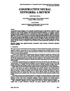
Figure 1 shows three samples of training processes. We find from Figure 1 that
0.05
0.12
0.14
0.115
0.135
0.045
Validation error
Validation error
0.04
0.035
0.03
0.11
0.13
0.105
0.125
0.1
0.12
0.095
0.115
0.09
0.11
0.085
0.105
0.025 0.08
0.1 0.02
0
100
200
300
400 Epochs
500
600
700
0.075
0
100
200
300
400 Epochs
500
600
700
800
0.095
0
100
200
300
400
500
600
700
800
Fig. 1. Three samples of training processes, breast cancer(left), diabetes (middle), heart disease (right). Each peak in this Figure represents the moment when a new NN was added to the ensemble. X-axis: the number of epochs, Y-axis: validation error.
when a new NN with one hidden node and random initial weights was added to the ensemble, there is a sharpe increase in the validation error. But eventually, with the increase of the number of both NNs and training epoches, the validation errors gradually reduced to a satisfactory level. This shows the NNE generally outperforms a single NN. Because the initial error of heart disease problem is quite small, at the first few training epochs, when adding untrained nodes, the validation error may be increased (right figure).
The ICNNE method is compared with some other approaches on three medical diagnosis databases in Table 2. The other data were obtained from [2].
Table 2. Compare the testing error of ICNNE with previous works, based 30 runs
ICNNE Mean SD CNNE[2] Mean SD EPNet[2] Bagging[2] Arc-boosting[2]
Breast Cancer Diabetes Heart disease 0.021 0.094 0.113 0.008 0.006 0.015 0.013 0.198 0.134 0.007 0.001 0.015 0.014 0.224 0.167 0.034 0.228 0.170 0.038 0.244 0.207
The results show that ICNNE can generally achieve better performance for most of the problems. ICNNE performs the best for diabetes and heart disease problems. But for breast cancer problem, CNNE is the best. Since the breast cancer problem is a relative easy one, it is difficult for ICNNE to further improve the result [2].
5
Conclusions
We have proposed an improved constructive algorithm to automatically design a near minimal NNE in this paper. In this approach, users only needed to specify two most important parameters (mh and r). Comparing with some previous work [2], less prior knowledge was requested from users, and a relative better performance was obtained.
References 1. Liu, Y., Yao, X.: Ensemble learning via Negative Correlation. Neural Networks, 12 (1999) 1399-1404 2. Monirual Islam, Md., Yao, X., Murase, K.: A Constructive Algorithm for Training Cooperative Neural Network Ensembles. IEEE Transactions on Neural Network, 4 (2003) 820-834 3. Liu, Y., Yao, X., Higuchi, T.: Evolutionary Ensembles with Negative Correlation Learning. IEEE Transactions on Evolutionary Computation, 4 (2000) 380-387 4. Blake, C.L., Merz, C.J.: UCI Repository of Machine Learning Databases [http://www.ics.uci.edu/ mlearn/MLRepository.html], Irvine, CA:University of California,Department of Information and Computer Science (1998)