An Iterative Procedure for Optimal Control of Bilinear Systems - arXiv

International Journal of Instrumentation and Control Systems (IJICS) Vol.2, No.1, January 2012

An Iterative Procedure for Optimal Control of Bilinear Systems H. Ramezanpour1, S. Setayeshi1, H. Arabalibeik2, A. Jajrami3 1

Amirkabir University of Technology, Tehran, Iran

[email protected], [email protected] 2

Research Center for Science and Technology in Medicine (RCSTIM), Tehran University of Medical Sciences, Tehran, Iran. [email protected] 3

Ferdowsi University of Mashhad, Mashhad, Iran [email protected]

ABSTRACT This paper presents a new and straightforward procedure for solving bilinear quadratic optimal control problem. In this method, first the original optimal control problem is transformed into a nonlinear twopoint boundary value problem (TPBVP) via the Pontryagin’s maximum principle. Then, the nonlinear TPBVP is transformed into a sequence of linear time-invariant TPBVPs using the homotopy perturbation method (HPM) and introducing a convex homotopy in topologic space. Solving the latter problems through an iterative process yields the optimal control law and optimal trajectory in the form of infinite series. Finally, sufficient condition for convergence of these series is proved by a theorem. Simplicity and efficiency of the proposed method is shown through an illustrative example.

KEYWORDS Bilinear systems, optimal control, homotopy perturbation method, Pontryagin’s maximum principle.

1.INTRODUCTION Bilinear systems are a special class of nonlinear systems, in which nonlinear terms are constructed by multiplication of control vector and state vector. An overview of the available control strategies for bilinear systems can be found in [1]-[5]. Besides, optimal control is one of the most active subjects in the control theory. Theory and application of optimal control have been widely used in different fields such as aircraft systems [6], robotic [7], biomedicine [8], etc. However, optimal control of nonlinear systems is a challenging task which has been studied extensively for decades. For solving nonlinear optimal control problems, indirect methods often lead to solving a Hamilton–Jacobi–Bellman (HJB) equation [9] or a nonlinear two-point boundary value (TPBVP) DOI : 10.5121/ijics.2012.2101

1


[10]. In general, an analytic solution does not exist for the HJB equation or nonlinear TPBVP, with the exception of the simplest cases. This has inspired researchers to present some approaches to obtain an approximate solution for the above-mentioned problems as well as obtaining an approximate optimal control for nonlinear systems. An excellent literature review on the methods for approximating the solution of HJB equation is provided in [11]. Besides, to approximate the solution of nonlinear TPBVPs, successive approximation approach (SAA) [12] and sensitivity approach [13] have been introduced recently. In those, a sequence of nonhomogeneous linear time-varying TPBVP’s is solved instead of directly solving the nonlinear TPBVP derived from the maximum principle. However, solving time-varying equations is much more difficult than solving time-invariant ones. The homotopy perturbation method (HPM) was initially proposed by the Chinese mathematician J. H. He [14-15]. This method has been widely used to solve nonlinear problems in different fields [16-18]. In contrast to the perturbation method [19], the HPM is independent upon small/large physical parameters in system model. However, like the other traditional nonperturbation methods, such as the Lyapunov’s artificial small parameter method [20] and Adomian’s decomposition method [21], uniform convergence of the solution series obtained via the HPM cannot be ensured. The main objective of this paper is to develop an optimal control design algorithm for a class of bilinear systems with a separated linear part. The algorithm is based on the HPM, where an iterative process is proposed to find a solution sequence of the nonlinear TPBVP, derived from the maximum principle. In this process, the nonlinear terms are considered as known additional disturbances so that the problem is transformed into a sequence of nonhomogeneous linear timeinvariant TPBVPs. The approach presented reduces the computational time and avoids the trouble of directly solving the nonlinear TPBVP or the HJB equation. A simulation example is employed to verify the validity of the suggested algorithm.

2.PROBLEM STATEMENT Consider a bilinear system of the form:

  n   x (t ) = Ax (t ) + Bu (t ) +  ∑ x j N j  u (t )   j =1    x (t0 ) = x0 where x ∈ R and u ∈ R n

m

are the state and control vectors respectively, A , B and N

(1)

j

are

constant matrices of appropriate dimensions with N j ∈ R n× m , and x 0 ∈ R n is the initial state vector. The objective is to find the optimal control law u ∗ (t ) that minimizes the following quadratic performance index (QPI):

J=

1 T 1 tf x (t f )Q f x (t f ) + ∫ ( xT (t )Qx (t ) + u T (t ) Ru (t ) ) dt 2 2 t0

(2)

subject to the system (1) where Q and Q f are symmetric positive semi-definite n × n matrices, and R is a symmetric positive definite m× m matrix. 2


According to the Pontryagin’s maximum principle, the optimality condition is obtained as the following nonlinear TPBVP:

 x (t ) = Ax(t ) − BR −1 BT  (t ) +  ( x(t ),  (t ) )  T  (t ) = −Qx(t ) − A  (t ) +  ( x(t ),  (t ) )   x(t0 ) = x0  (t ) = Q x(t ) f f  f

(3)

T   n   n  − 1  ( x(t ),  (t ) ) = − BR  ∑ x j N j   (t ) +  ∑ x j N j  w( x(t ),  (t ) )  j =1   j =1            n  ∂ 1  ( x(t ),  (t ) ) = −  wT ( x(t ),  (t ) )Rw( x(t ),  (t ) ) + T  B +  ∑ x j N j   z ( x)   j =1    ∂x  2        T    n    n   z ( x) = − R −1  B +  ∑ x j N j   B +  ∑ x j N j    j =1    j =1           w( x(t ),  (t ) ) = z ( x) (t )

(4)

in which:

and

 ∈ Rn is the co-state vector. Also the optimal control law is given by: u ∗ (t ) = − w( x (t ),  (t ) )

(5) Unfortunately, it is difficult to solve problem (3) even numerically. To overcome this difficulty, we will use the HPM in the next section, which transforms problem (3) into a sequence of linear time-invariant TPBVPs. Solving the latter problems recursively and intercepting frontal N terms of the series solution, a suboptimal solution is obtained.

3. PROPOSED METHOD Let us define the operators F1[ x(t ), (t )] and F2 [ x(t ),  (t )] as follows: ∆

F1[ x(t ),  (t )] = x (t ) − Ax(t ) + BR −1BT  (t ) −  (x(t ),  (t ) ) ∆

F2 [ x(t ),  (t )] = (t ) + Qx(t ) + AT  (t ) − (x(t ),  (t ) ).

(6) (7)

From (3) it is obvious that:

 F1[ x (t ),  (t )] = 0   F2 [ x (t ),  (t )] = 0

(8)

The operators F1 and F2 can generally be divided into two parts, a linear part and a nonlinear part. Therefore, we can write:

3


 F1 [ x ( t ),  ( t )] = L1 [ x ( t ),  ( t )] + N 1 [ x ( t ),  ( t )]   F2 [ x ( t ),  ( t )] = L2 [ x ( t ),  ( t )] + N 2 [ x ( t ),  ( t )]

(9)

where Li and N i are the linear and nonlinear parts of Fi for i = 1,2 respectively. Now, we

x (t, p) : [t0 , t f ] × [0,1]  → R and construct two homotopies in topologic space for (9), ~ ~

 ( t , p ) : [t 0 , t f ] × [0,1]  → R , which satisfy the following equation:  L1[( x (t , p ),  (t , p )) − ( xini (t ), ini (t ))] + pL1[ xini (t ), ini (t )] + pN1[ x (t , p ),  (t , p )] = 0   L2 [( x (t , p ),  (t , p )) − ( xini (t ), ini (t ))] + pL2 [ xini (t ), ini (t )] + pN 2 [ x (t , p ),  (t , p )] = 0

(10)

with the boundary conditions:

~x (t , p ) = x , ~ (t , p ) = Qx (t ) 0 0 f f

(11)

where p ∈ [0,1] is an embedding parameter which is called homotopy parameter, ini (t ) and

xini (t ) are the initial guesses for the solution of (3), i.e.  (t ) and x(t ) respectively. Setting p = 0 and p = 1 in (10) yields:  L1[( x (t , 0),  (t , 0)) − ( xini (t ), ini (t ))] = 0  x (t , 0) = xini (t ) p=0⇒ ⇒    L2 [( x (t , 0),  (t , 0)) − ( xini (t ), ini (t ))] = 0  (t , 0) = ini (t )

(12)

~  F [ ~ x (t ,1),  (t ,1)] = 0 p =1 ⇒  1 ~  F2 [ ~ x (t ,1),  (t ,1)] = 0

(13)

~ x (t, p) and  (t , p ) Therefore, if the homotopy parameter p changes from zero to unity, ~ change from the initial guesses xini (t ) and ini (t ) to the exact solution of (13). In topology we call it deformation. Obviously, when p = 1, TPBVP (10)-(11) is equivalent to the nonlinear TPBVP (3).

3.1 Discussion on L and Initial guesses It should be mentioned that we have a great freedom to choose linear operators and initial guesses. Once one chooses these parts, the homotopy equation is completely determined, because the remaining part is actually the original equation (see (10)) and we have less freedom to change it. Here we discuss some general rules that should be noted in choosing linear operators and initial guesses. According to the homotopy perturbation procedure, L should be easy to handle and closely related to the original equation. We mean that it must be chosen in such a way that one has no difficulty in subsequently solving systems of resulting equations. Strictly speaking, in constructing L , it is better to use some part of the original equation. A suitable choice of linear operators can be as follows: 4

International Journal of Instrumentation and Control Systems (IJICS) Vol.2, No.1, January 2012 ∆ ∂~ ~ x (t , p ) ~  ~ L [ x ( t , p ),  ( t , p )] = − A~ x (t , p ) + BR −1 B T  (t , p ) 1  ∂t  ~ ∆ ~ ∂ (t , p ) ~ L [ ~ x (t , p ),  (t , p )] = + Q~ x (t , p ) + AT  (t , p )  2 ∂t

( 14)

There is no universal technique for choosing the initial guess in most iterative methods; but from previous works done on HPM and our own experiences, we can conclude that the initial guess should be obtained from the original equation and reduce complexity of the resulting equations. For example, it can be chosen to be the solution to some part of the original equation, or it can be chosen from boundary conditions. One suitable choice can be the solution of the following linear TPBVP, which comes from the original TPBVP (3):

 L1[ xini (t ), ini (t )] = 0   L2 [ xini (t ), ini (t )] = 0  x (t ) = x ,  (t ) = Qx(t ). 0 ini f f  ini 0

(5)

Now the following theorem is presented, which indicate how to use the HPM in practice for handling TPBVP (3): Theorem 3.1. The solution of nonlinear TPBVP (3) can be written as x(t ) =

∞

∑x

(n)

(t ) and

n =0

∞

 (t ) = ∑ ( n ) (t ) , where the n-th order terms x ( n ) ( t ) and ( n ) ( t ) for n ≥ 0 are achieved n =0

recursively by solving a sequence of linear time-invariant TPBVPs.

~ x (t, p) and  (t , p ) Proof. Assume that the embedding parameter p is a small parameter and ~ ~ x (t, p) and  ( t , p ) as are infinitely differentiable with respect to p around p = 0 . Expanding ~ Maclaurin series yields:

 ~ x (t , p ) = x ( 0 ) (t ) + x (1) (t ) p + x ( 2 ) (t ) p 2 +  (16) ~  (t , p ) = ( 0 ) (t ) + (1) (t ) p + ( 2 ) (t ) p 2 +  ~ 1 ∂ n  (t , p) 1 ∂ n x (t, p ) (n)  ( t ) = where x (n ) (t ) = and . Substituting (15) in (10), n ! ∂p n n ! ∂p n p = 0 p =0 rearranging with respect the order of p , and equating terms with the same order of p on each side we obtain:

 L1[( x(0) (t ),  (0) (t ))] − L1[ xini (t ), ini (t )] = 0  p 0 :  L2 [( x (0) (t ),  (0) (t ))] − L2 [ xini (t ), ini (t )] = 0  (0) (0)  x (t0 ) = x0 , x (t f ) = x f

(17a)

5


 L1[ x (1) (t ),  (1) (t )] + L1[ xini (t ), ini (t )] + h1(0) (t ) = 0  p1 :  L2 [ x (1) (t ),  (1) (t )] + L2 [ xini (t ), ini (t )] + h2(0) (t ) = 0  (1) (1)  x (t0 ) = 0, x (t f ) = 0

(17b)

  L1 ( x ( n ) (t ),  ( n ) (t )) + h1( n −1) (t ) = 0  L ( x ( n ) (t ),  ( n ) (t )) + h2( n −1) (t ) = 0 n  2 p :  (n) (n)  x (t0 ) = 0 , x (t f ) = 0 n ≥ 2 

(17c)

where nonhomogeneous terms h1( n−1) (t ) and h2( n−1) (t ) are calculated using the information obtained from previous steps as follows:

h1( n −1) (t ) =

 1  ∂ n −1  n −1 (N 1 ([ x ( 0 ) + px (1) + p 2 x ( 2 ) + ...] , [( 0 ) + p(1) + p 2 ( 2 ) + ...])) (18) ( n − 1)!  ∂p  p =0

h2( n −1) (t ) =

 1  ∂ n −1  n −1 (N 2 ([ x ( 0 ) + px (1) + p 2 x ( 2 ) + ...] , [( 0 ) + p(1) + p 2 ( 2 ) + ...]))( ( n − 1)!  ∂p  p =0 19)

Therefore, at each step, we obtain a nonhomogeneous linear time-invariant TPBVP which should be solved in a recursive manner. After obtaining x( n) (t ) and  ( n ) (t ) for n ≥ 0 , we should set p = 1 in (16) to obtain the exact solution of problem (3). Setting p = 1 in (16) yields:

 x(t ) = ~ x (t ,1) = x ( 0) (t ) + x (1) (t ) + x ( 2) (t ) +   ~  (t ) =  (t ,1) = ( 0) (t ) + (1) (t ) + ( 2) (t ) + 

(20)

and the proof is complete. Remark 3.1. It should be noted that series in (20) converge rapidly for most cases; however, convergence rate depends upon the nonlinear operators. As this method is an iterative method, so the Banach’s fixed point theorem can be applied for convergence study of the series (20).

~  N1 [ ~ x (t, p),  (t, p)] Theorem 3.2. (Sufficient condition of convergence) Suppose that N =   ~ ~  N 2 [ x (t, p),  (t, p)] ∆  x(t )  and z =  and X and Y are Banach spaces and N : X → Y is a contractive nonlinear  (t ) ∆

mapping that is 6


∀w , w ∗ ∈ X ; N ( w ) − N ( w ∗ ) ≤  w − w ∗ , 0 <  < 1 Then according to Banach’s fixed point theorem N has a unique fixed point z that is N ( z) = z . The sequence generated by the HPM may be regarded as

Wn = N (Wn −1 )

n −1

Wn −1 = ∑Wi

,

,

n = 1,2,3,...

i =0

{

}

And suppose that W0 = w0 ∈ Bt ( w) where Bt ( w) = w∗ ∈ X w∗ − w < t ∈ [t0 , t f ] , then we have

(i ) Wn ∈ Bt ( w) (ii ) lim Wn = w n →∞

Proof. (i) By inductive approach, for n = 1 we have

W1 − w = N (W0 ) − N ( w) ≤  w0 − w n −1 w0 − w , as an induction hypothesis, then Assume that Wn −1 − w ≤ 

Wn − w = N (Wn −1 ) − N ( w) ≤  Wn −1 − w ≤  n w0 − w . Using (i) we have

Wn − w ≤  n w0 − w ≤  n t ≤ t ⇒ Wn ∈ Bt ( w) n n (ii) Because of Wn − w ≤  w0 − w and lim  = 0 , lim Wn − w = 0 , that is, lim Wn = w

n→∞

n→∞

n→∞

and proof is complete. Remark 3.2. Substituting (20) in (4), the optimal control law is obtained as follows: ∞

u ∗ (t ) = − R −1 B T ∑  ( n ) (t ).

(21)

n =0

4. CASE STUDY The bilinear model of a chemical reactor [5] is given by:

 13  6 A=  − 50  3

5  12   8 −  3 

,

 1 − B =  8    0 

,

 −1 N1 =   0

,

0 N2 =   0 

The normalized state variable x1 and x2 represent temperature and concentration of the initial product of the chemical reaction, respectively. The normalized scalar control u represents the cooling flow rate in a jacket around the reactor. The objective is to transfer the system in a finite time very closely to the origin. Weighting matrices are chosen as follows: 7


0  1000 F =   0 1000

,

10 0  Q=   0 10

,

R =1

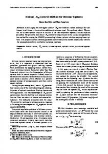
Initial conditions are x (0) = x0 = [0.15 0]T and t f = 3 . Simulation results for three iterations are presented in Figs. 1, 2 and 3, which show achieving desired goals.

Fig 1. Profiles of temperature

Fig 2. Profiles of Concentration

8


Fig 3. Control Input

5. CONCLUSION In this paper, based on the HPM, an efficient iterative method has been introduced for optimization of bilinear control systems. In this method, by introducing a recursive process, the optimal control law is determined in the form of infinite series with easy-computable terms. The proposed method avoids directly solving the nonlinear TPBVP or the HJB equation. In addition, despite of the successive approximation approach [12] and sensitivity approach [13], it avoids solving a sequence of linear time-varying TPBVPs. It only requires solving a sequence of linear time-invariant TPBVPs. Therefore, in view of computational complexity, the proposed method is more practical than the above-mentioned approximate methods.

REFRENCES [1] [2] [3] [4] [5] [6]

R. Mohler, Natural Bilinear Control Processes, New York: Academic, 1973. R. Mohler, "Natural Bilinear Control Processes," IEEE Trans. Syst. Sci. Cybern., vol. SSC-6, pp. 192-197, 1970. C. Bruni, G. DiPillo, and G. Koch, "Bilinear Systems: appealing class of "Nearly Linear" systems in theory and applications," IEEE Trans. Automat. Contr., vol. AC-19, pp. 334-348, 1974. A. Benallou, D. A. Mellichamp, and D. E. Seborg, "Optimal Stabilizing controllers for bilinear systems," Int. J. Contr., vol. 48, pp. 1487-1501, 1988. E. Hofer and B. Tibken, "An Iterative method for the finite-time bilinear quadratic control problem," J. Optim. Theory Applications, vol. 57, pp. 411-427, 1988. W. L. Garrard and J. M. Jordan, “Design of nonlinear automatic flight control systems,” Automatica, vol. 13, no. 5, pp. 497-505, 1977.

9

International Journal of Instrumentation and Control Systems (IJICS) Vol.2, No.1, January 2012 [7]

[8] [9] [10] [11] [12] [13] [14] [15] [16] [17]

[18]

[19] [20] [21]

S. Wei, M. Zefran, and R. A. DeCarlo, “Optimal control of robotic system with logical constraints: application to UAV path planning,” IEEE International Conference on Robotic and Automation, Pasadena, Ca, Usa, 2008. M. Itik , M. U. Salamci, and S. P. Banksa, “Optimal control of drug therapy in cancer treatment,” Nonlinear Analysis, vol. 71, pp. 473-486, 2009. R. Bellman, On the theory of dynamic programming, P. Natl. Acad. Sci. USA, vol. 38, no. 8, pp. 716-719, 1952. L. S. Pontryagin, Optimal control processes, Usp. Mat. Nauk, vol. 14, pp. 3-20, 1959. R. W. Beard, G. N. Saridis, and J. T. Wen, Galerkin approximations of the generalized HamiltonJacobi-Bellman equation, Automatica, vol. 33, no. 12, pp. 2159-2177, 1997. G. Y. Tang, “Suboptimal control for nonlinear systems: a successive approximation approach,” Syst. Control Lett., vol. 54, no. 5, pp. 429-434, 2005. G. Y. Tang, H. P. Qu, and Y. M. Gao, “Sensitivity approach of suboptimal control for a class of nonlinear systems,” J. Ocean Univ. Qingdao, vol. 32, no. 4, pp. 615-620, 2002. J. H. He, “Homotopy perturbation technique,” Computational Methods in Applied Mechanics and Engineering, vol. 178, pp. 257–262, 1999. J. H. He, “A coupling method of a homotopy technique and a perturbation technique for non-linear problems,” International Journal of Non-Linear Mechanics, vol. 35, pp. 37–43, 2000. J. H. He, “Homotopy perturbation method for solving boundary value problems,” Phys. Lett. A, vol. 350, pp. 87–88, 2006. D. D. Ganji and A. Sadighi, “Application of He’s homotopy perturbation method to nonlinear coupled systems of reaction–diffusion equations,” Int. J. Nonlinear Sci. Numer. Simul., vol. 7, pp. 411–418, 2006. M. Rafei and D. D. Ganji, “Explicit solutions of Helmholtz equation and fifth-order KdV equation using homotopy perturbation method,” Int. J. Nonlinear Sci. Numer. Simul., vol. 7, pp. 321–328, 2006. J. A. Murdock, Perturbations: Theory and Methods, Classics in Applied Mathematics, vol. 27, SIAM, 1999. A. M. Lyapunov, General Problem on Stability of Motion, Taylor & Francis, London, 1992 (English translation). G. Adomian, and G. E. Adomian, A global method for solution of complex systems, Math. Modelling, vol. 5, no. 4, pp. 251-263, 1984.

10