8050 Zürich, Switzerland. A.Puzenko, Y. Ryabov, and Y. Feldman. Department of Applied Physics. The Hebrew University of Jerusalem. Jerusalem 91904, Israel.
IEEE Transactions on Dielectrics and Electrical Insulation
Vol. 13, No. 2; April 2006
247
An RCL Sensor for Measuring Dielectrically Lossy Materials in the MHz Frequency Range 1. Comparison of Hydrogel Model Simulation with Actual Hydrogel Impedance Measurements M.S. Talary, F. Dewarrat, A. Caduff Solianis Monitoring AG. 8050 Zürich, Switzerland
A.Puzenko, Y. Ryabov, and Y. Feldman Department of Applied Physics The Hebrew University of Jerusalem Jerusalem 91904, Israel
ABSTRACT There is a requirement for the development of non-invasive continuous blood glucose monitoring devices to meet the clinical demands of the rapidly increasing number of people currently developing diabetes mellitus. Impedance Spectroscopy is a technology that meets the requirements of such devices. An NI CGMD is being developed as a device that couples a sensor to the skin to form an RCL sensor. The reliability of such an RCL sensor model has been investigated by comparing electrodynamical simulations to in-vitro measurements of dielectrically “lossy” materials. The sensor has been modeled and simulated in FEMLAB (Finite Element Modeling Laboratory). In-vitro measurements are performed on hydrogels, representing the lossy material, by the aid of a Rohde & Schwarz VNA (vector network analyzer). From the quantitative agreement of the results we conclude, that the proposed qualitative model is appropriate for the characterization of the RCL sensor and suggests that more detailed models can be used to elucidate the behavior of human skin tissue. Index Terms - Equivalent circuits, circuit simulation, transducers, dielectric measurements, dielectric materials, skin, medical diagnosis.
1 INTRODUCTION DIABETIS mellitus is a metabolic disease that can lead to uncontrolled glucose excursions. There is an increasing interest in the closer monitoring of glycaemic conditions to reduce the incidence of complications associated with prolonged hyper or hypo-glycaemic excursions, preferably in a non-invasive and continuous manner. Due to the known specific reactions of blood and tissue cells on a varying glucose concentration, the electrolyte balance across membranes of cells in blood and underlying tissue is changed as a function of glucose. Dielectric spectroscopy (DS) or Impedance Spectroscopy (IS), as a more recognized term in the bio-impedance community, is thought to be sensitive to these subtle changes. In this work, we investigate the Manuscript received on 19 July 2005, in final form 26 October 2005.
feasibility of using DS techniques to monitor changes in complex human biological systems due to the alteration in blood glucose levels. It has been previously reported that a non-invasive, continuous glucose monitoring device (NI-CGMD) is being developed using impedance spectroscopy to provide real time monitoring of glucose levels in human tissue [1]. This NI-CGMD consists of a sensor capacitively coupled to the body, a signal generator operated in a selected frequency range (1 – 200 MHz) and a microprocessor that controls the operation of the device. The sensor has the surface area of a wristwatch and consists of an open resonant circuit coupled to the skin (see Figure 1). The mode of interaction of an applied electromagnetic field with the skin depends on a number of factors such as the design of the sensor, the frequency of the applied electric field and changes in the dielectric properties of the underlying tissue. These factors
1070-9878/06/$20.00 © 2006 IEEE
248
M.S. Talary et al.: An RCL Sensor for Measuring Dielectrically Lossy Materials in the MHz Frequency Range
can be investigated by developing an artificial model of human tissue using hydrogels. The dielectric properties of the hydrogel can be designed to reflect the biophysical properties of skin as a simplified artificial model by taking advantage of its high water content. NI-CMGD
L
achieved by applying a suitable force to the sensor on the hydrogel surface and ensuring that the hydrogel surface is smooth. All the measurements were performed using a Vector Network Analyzer in the frequency range 1 - 200 MHz. The applicability of the approach of using hydrogels as a skin model and the feasibility of using the NI-CGMD for measuring dielectric changes in the materials are also confirmed in this work.
2 HYDROGELS
C,R
Hydrogel as artificial model of skin tissue
Figure 1. Diagram showing a schematic of the NI-CMGD sensor capacitively coupled to skin. Here the sensor coupled to skin and under-lying tissue can be considered as a lump capacitance element C in parallel with the resistance R and L is external inductance.
Estimations of the wave phase incursion kl in the different sub domains of the system sensor-body where;
k=
2π f c
ε,
where f is frequency in Hz c = 3 x 10⁸ m/s , ε is the dielectric permittivity of the subdomain and l is its linear size ) show that the electromagnetic wave propagation processes can be neglected ( kl 0 while C ij < 0 , however the signs of these coefficients reflect the signs of the charges accumulated on the conductors. Thus, if we want to know only the capacitances then only the absolute values of
Cij have to be used in further consideration. In
C11 is the “grounded” capacitance of the central strip, C 22 is the
the case of the NI-CGMD sensor (see Figure 2),
“grounded” capacitance of surrounding “ring” and the shield, and
C12 = C 21 is their mutual capacitance. Note that when calculating Cii , the “ground” has to be modelled as an additional electrode far enough from the sensors electrode with a zero potential in order to have a minimal impact on the field distribution near the NI-CGMD surface To evaluate the properties of the NI-CGMD sensor with respect to the direct currents, a similar approach can be applied as follows: k
I i = ∑σ i, j V j
(11)
j =1
where
V j is the potential of jth conductor, I i is total current
through the surface of the ith conductor of and conductivity
coefficients
and
resistance
σ i, j are the
coefficients
are
Rij = 1 / σ ij . This approach of ‘conductivity coefficients’ is R
based on the complete analogy between equations (2-4) for ES problem and equations (6-8) for DC problems. An extended equivalent circuit for the NI-CGMD sensor, in which all capacitance and resistance coefficients are taken into account, is shown in Figure 4.
C
Equivalent circuit of
+ Figure 3. The simplified equivalent circuit of NI-CGMD sensor attached to the sample.
However, this simplified model is not able to describe quite complicated details of the electrostatic behaviour of the sensor attached to the body. This is the reason that our simulations of the electrostatic properties of the NI-CGMD sensor were based on the well-known approach of capacitance coefficients [8]. For the system of k conductors situated in any dielectric medium it is possible to establish the following relationship k
Qi = ∑ C i , j V j
(10)
R11
R12
C11
C12 R22
C22
-
j =1
Here V j is potential of jth conductor, th
on the surface i conductor of
Qi is charge accumulated
C i , j are the so-called capacitance
Figure 4. Extended equivalent circuit for the NI-CGMD sensor.
IEEE Transactions on Dielectrics and Electrical Insulation
Vol. 13, No. 2; April 2006
251
3.3 THE GLASS COATING LAYER
3.4 SIMULATION OF THE NI-CGMD SENSOR COUPLED TO HYDRO-GELS
In the real NI-CGMD sensor, the sensor and electrodes are coated with a very thin glass layer to protect the electrodes from physical damage in use and provides a fixed parasitic capacitance that should be considered in the effective model of the sensor when in contact with the skin. This thin layer has a comparatively
Let us consider now the NI-CGMD sensor with the glass coating layer, terminated in series to an inductance L, as in the real measurement system [1]. In this case, we accept the entire equivalent circuit of the measuring device attached to any material
C c and a very high resistance Rc due to the fact
The simulation procedure and impedance calculation of this equivalent circuit has to be implemented according to the protocol presented in Table 2. The modulus of the impedance value has to be calculated according to the following equations (14-15):
big capacitance
that it is made from a material with negligible conductivity. For this reason we can neglect
Rc → ∞ in the resulting equivalent
circuit that is presented in Figure 5.
under investigation as presented in Figure 5 (where Rc
Z = iωL + Z i, j =
Rc
Cc
Z ( Z + Z 22 ) 1 + 12 11 iωC c Z11 + Z 22 + Z12
R12
C11
R22
C22
(14)
Ri , j
(15)
1 + iωCi , j Ri , j
Where the cyclic frequency
R11
→ ∞ ).
ω = 2π f . Note that in the
simulations, in addition to the conductors #1 and #2 we introduced an additional conductor on top of the simulation geometry. This conductor approximates the “ground” at infinity. As described previously, this conductor is used in order to simulate the impact of the “grounded” capacitances and the currents, which are going to the infinity. Otherwise the simulation algorithm will not be able to evaluate these effects since there is a constraint of total zero charge for all the conductors involved in the electrostatic simulation, and the constraint of total compensation for all currents
C12
in the direct currents simulation. Thus, in order to get the
Ci , j
values for some particular model, it is necessary to perform two simulation processes (Step I and Step II in Table 2). Having completed the simulation processes, the post-processing tool of FEMLAB can be used to evaluate the values of Figure 5 Equivalent circuit of the NI-CGMD sensor. For the real measuring system in a frequency range higher than 100 Hz one can neglect the resistance of the coating layer.
According to the effective circuit presented in Figure 5, the capacitance of this coating layer can be evaluated as:
Cc =
C eq (C12 (C11 + C 22 ) + C11C 22 ) C11C 22 − (C11 + C 22 )(C eq − C12 )
C eq = C12 '+ where all the coating layer.
C11 ' C 22 ' C11 '+C 22 '
(12)
(13)
C i , j ' are obtained from the simulations with the
C1r,1 , − C1r, 2 by
integrating over the surfaces of Conductor #1 and Conductor #2 respectively. The values of
C ir, j are different from the true values of C i , j
since our simulations are in 2D. Therefore, the surface integration in the post-processing tool implies that the simulation geometry is simply extended in the third dimension for 1 m. Thus, to get an estimation of
C i , j we rescale the C ir, j values with the actual
length of the central strip, which is 24 mm in the case of the sensor described in previous work [1] such that:
C i , j = 0.024 C ir, j and derives the values
(16)
C 2r, 2 , − C 2r,1 via the integration over the
surfaces of conductor #1 and conductor #2 respectively.
252
M.S. Talary et al.: An RCL Sensor for Measuring Dielectrically Lossy Materials in the MHz Frequency Range
Table 2. The process steps for simulations of both electrostatic and direct current procedure.
ES and DC (two runs with different Boundary conditions)
Boundary conditions for the NI-CGMD sensor
I)
Calculation
of
C i , j values
First run Conductor #1 U=1 [V] Conductor #2 U=0 [V] Ground at the infinity U=0 [V] Second run Conductor #1 U=0 [V] Conductor #2 U=1 [V] Ground at the infinity U=0 [V]
without a coating layer
II) Calculation of
Ri , j values
without a coating layer
IV) Calculation of
C c to calculate the impedance value for the equivalent circuit presented in Figure 5.
C eq (C12 (C11 + C 22 ) + C11C 22 ) C11C 22 − (C11 + C 22 )(C eq − C12 )
C eq = C12 '+
Z = iω L + Zi, j =
C11 [pF]
C 22 [pF]
C12 [pF]
C c [pF]
19.57
38.76
12.48
582.97
Table 4. The parameters of hydro-gel samples for the simulation input and the resulting simulation values of the resistances.
Hydro-Gel
C11 ' C 22 ' C11 '+C 22 '
1 Z ( Z + Z 22 ) + 12 11 iωCc Z11 + Z 22 + Z12
Ri , j 1 + iωCi , j Ri , j
Then using (16) it is possible to calculate
(17)
Table 3. The capacitances of the NI-CGMD sensor attached to the hydro gel sample with dielectric permittivity ε=63.
The same Boundary conditions
Cc =
1 0.024 σ r i , j
Four different hydrogel samples were measured with the NICGMD sensor in the frequency range 1-100 MHz at 25°C. The hydrogels had the same dielectric permittivity ε=63, but different values of conductivity as shown in Table 1. The simulations for the NI-CGMD sensor attached to the same compositions of hydrogels (Table 1) were processed according to the routine described above. The values of the capacitances and resistances evaluated by simulation of the different samples of hydrogels are presented in Tables 3 and 4.
First run Conductor #1 U=1 [V] Conductor #2 U=0 [V] Ground at the infinity U=0 [V] Second run Conductor #1 U=0 [V] Conductor #2 U=1 [V] Ground at the infinity U=0 [V]
and
C i , j , Ri , j and
σ 1r,1 , − σ 1r, 2 , σ 2r, 2 and − σ 2r,1 . As with
4.1 COMPARISON OF RESULTS OF SIMULATION WITH ACTUAL HYDROGEL MEASUREMENTS
The same Boundary conditions
with a coating layer
VI) Taking into account all
evaluate the values of
4 RESULTS AND DISCUSSION
Ri , j values
V) Calculation of coating capacitance Cc
Using the post processing tool of FEMLAB it is possible to
Ri , j =
with a coating layer of
Ri , j values.
calculation of the capacitances one needs to rescale the conductance. Thus:
Ci′, j values
III) Calculation
of boundary conditions is used for calculation of
C 2, 2 and
C 2,1 = C1, 2 . The similar routine with two processes and two sets
1 2 3 4
σ [Sm/m]
R11 [Ω]
R22 [Ω]
0.30 0.35 0.44 0.51
132.33 113.42 90.22 77.84
60.67 52.00 41.36 35.69
R12 [Ω] 304.07 260.63 207.32 178.86
The averaged results from the three actual hydrogel measurements using a VNA and simulations in terms of the impedance modulus are presented in Figure 6, where the value of the inductance in the NI-CGMD Sensor is taken to be L=270 nH. The Figures 6 (a) and (b) show that the simulated results are in fair qualitative agreement with the actual experimental data. Therefore, we can conclude that the ideology of the simulation model and the equivalent circuit designed for the NI-CGMD sensor are in close agreement with the operation of the real measuring device. The quantitative disagreement between the simulations and the experimental results are largely due to the 2D
IEEE Transactions on Dielectrics and Electrical Insulation
Vol. 13, No. 2; April 2006
approximation used in the simulation, since the capacitances and resistances evaluated in 2D cannot be simply rescaled in the 3D case as presented in equations (16) and (17). Moreover, the simulation results presented in Figure 6(b) exhibit linear increase in
Z with frequency in the high frequency range while the
experimental data in Figure 6(a) show a remarkably non-linear increase in this same frequency region. Note in this regard that the linear increase in the simulated
Z is due to the term iωL in
equation (14). Thus, the deviation from the linear behaviour found in the experimental data implies that, in addition to the “external” inductance L, the real sensor has its own inductive properties, which cannot be evaluated by the approximation of static currents used in this model.
253
4.2 SENSITIVITY In order to evaluate the glucose concentration in skin, underlying tissue and blood, the NI-CGMD sensor tracks the position of the impedance modulus minimum. The curves in Figures 6 (a) and (b) show the frequency dependencies of the impedance modulus correspondent minimum:
Z for the different hydrogel samples. The
coordinates
f min and Z
of
the
impedance
modulus
for both simulation and experimental
min
data are presented in Figures 7 and 8, respectively. 60
F Sim F Exp
55 50
fmin MHz
45
a) 180 170
IZI IZI IZI IZI
160 150
0.4 0.5 0.65 0.8
35 30 25
140
20 0.3
130
IZI Ohn
40
120
0.4
0.5
0.6
0.7
0.8
0.9
Concentration
110 100
Figure 7. Dependencies of
90
f min on the electrolyte concentration of the
hydrogel samples. Filled and open symbols correspond to the simulated values and experimental data respectively.
80 70 60 10
20
30
40
50
60
70
80
90
80
100
IZI Sim IZI Exp
78
f MHz
76
b)
74
180
72
160
IZI Ohn
150
IZImin Ohm
IZI 0.4 IZI 0.5 IZI 0.65 IZI 0.8
170
70 68
140
66
130
64
120
62
110
60 0.3
100 90
0.4
0.5
0.6
0.7
0.8
0.9
Concentration
80 70
Figure 8. Dependencies of Z
60 10
20
30
40
50
60
70
80
90
100
f MHz
averaging over three experimental runs for every concentration (NaCl=0.4; 0.5; 0.65; 0.8 %)
on the electrolyte concentration of the
hydrogel samples. Filled and open symbols correspond to the simulated values and experimental data respectively.
With regards to Figure 6. Experimental (a) and simulated (b) values of Z obtained by
min
Z
min
, it is essential to investigate its
“parabolic” like dependence on the electrolyte concentration of the hydrogel samples. The shape gives us an idea that in the region of concentrations between 0.5 - 0.6 % NaCl, the measuring device has low sensitivity to the changes in conductivity hence
Z
min
.
254
M.S. Talary et al.: An RCL Sensor for Measuring Dielectrically Lossy Materials in the MHz Frequency Range
Moreover, even outside this region, due to the nature of the inverse “parabolic” shape of the function, certain values of
Z
min
300
obtained from two essentially different values of electrolyte concentrations in the hydrogels. For example, in Figure 8 from the
Z
min
curve one finds for Z
= 77 Ohm two
min
different correspondent values of concentrations. The results presented in Tables III and IV show that the electrolyte concentration of the hydrogel strongly affects the measured conductivity but is not affecting changes in permittivity of the sample (i.e. there is a big impact on the resistances is no influence on capacitances
250
= 61.96 MHz
fi
200
IZIi = 128.46 Ohm
IZI
experimental
R series
A)
can be
150
Ri , j and there
100
C i , j ).
10
20
30
40
50
60
70
80
90
100
110
100
110
f MHz 300
4.3 INTERSECTION POINT
C series
B) 250
200
IZI
Figures 6 (a) and (b) can be seen to describe another interesting phenomenon – all the curves obtained for different hydrogel samples intersect at one point. The nature of this intersection could be investigated in the frame of the simplified equivalent circuit of the NI-CGMD sensor (see Figure 5). Note that in this circuit R and C are the equivalent sensor resistance and capacitance estimated from the static ES and DC simulations, and L is the external inductance included in the measuring setup L=330 nH. Thus, the impedance of this equivalent circuit is:
150
100
50 10
Z = i 2π f L +
R 1 + i 2π f RC
1 + 2η 2 − η 2
(
2
(19)
(20)
)
60
70
80
90
scheme presented in Figure 5. The thick curves in both panels are obtained for L = 330 nH , C = 10 pF and R = 304 Ohm . The curves in the panel (a) were calculated for the constant
C = 10 pF by variations of R. R = 304 Ohm
The curves in the panel (b) were obtained for the constant by variations of C.
Where the coordinates of this modulus minimum at resonance are:
= ρ 2 1 + 2η 2 − 1 − η 2 , for
50
Figure 9. The frequency dependencies of Z calculated for the equivalent
2
min
40
(18)
2π f R2C R Z= + 2π f L − 2 2 ( ) ( ) f RC f RC + 1 2 1 + 2 π π
Z
30
f MHz
The method previously described measures the modulus of this impedance, which is:
f min = f 0
20
f = f min . (21)
1 ρ Here η = , ρ = L / C and f 0 = R 2π LC is resonance frequency of circuit (for R=0). The variations of R and C values lead to two sets of curves as presented in Figure 9.
The existence of the intersection point implies that there are variations in the resistance R at the constant C, since variations in C remove this intersection point. Thus, the presence of the intersection point in the experimental hydrogel measurements using the NI-CGMD sensor reflects the fact that the capacitances and consequently the dielectric permittivity in these measurements are constant. In general, the absence of the intersection point means that there are changes in the capacitances and dielectric permittivity of the sample. Coordinates of the intersection point
f i and Z i can be obtained by using equation (19) as solution of the equation
2 π fi =
∂Z ∂R
ω0 2
= 0: f = fi , Z = Z
i
(22)
IEEE Transactions on Dielectrics and Electrical Insulation
Vol. 13, No. 2; April 2006
255
Note that in comparison to the equations (24-25) with equations
ρ 2
Zi =
(23)
ω 0 = 1 / LC is the cyclic resonance frequency of
Where
ρ = L / C its wave resistance. Thus, the
ideal LC-tank and
intersection point could be treated as a frequency point where the NI-CGMD sensor reaches a “matched line” condition. Equations (22-23) can be converted to obtain the relationships:
1 C= 4π f i Z L=
Z
(24) i
(25)
2π f i
f i = 61.96 MHz and Z i = 128.46 Ω , which with the help equations
C = 9.998 pF
(24-25) gives L = 329.97 nH and that are in perfect agreement with the values
used for the simulations (see caption for Figure 9). One can do the similar calculations for the equation (14) and get that for the equivalent scheme proposed in Figure 5
2π f i =
where
C c + 2C 0 2C c C 0 L Cc L 2C c C 0 + 4C 02
Zi =
C 0 = C1, 2 +
C1,1C 2, 2 C1,1 + C 2, 2
(26)
(27)
is the capacitance of the
C c of the glass-coating layer much higher than C 0 ,
and then equations (26-27) obtain the form similar to equations (22-23). In other words if the thickness of the glass coating vanishes then one gets that the equivalent scheme in Figure 5 similar to one presented in Figure 4. Inverting equations (26-27) one gets
1 Cc = 2π f i (2π f i L − Z i ) C0 =
1 4π f i Z
However, it seems not to be a problem since the value of L is fixed by the design. For example in the case of the simulations presented in this report L=270 nH,
C 0 = C1, 2 +
C1,1C 2, 2 C1,1 + C 2, 2
C c = 582.97 pF and
= 25.48 pF (see data from Table
3). The intersection point for the same simulation data in Figure 7(b) is
f i = 44.72 MHz and Z i = 69.75 Ω , which with
the help of equations (28-29) gives
(28)
(29) i
7(a) one gets
C c = 581.93 pF and
f i = 47.44 MHz Z i = 78.59 Ω which with
the help of equations (28-29) gives
C c = 1775 pF and
C 0 = 21.34 pF . Equations (28-29) provide us with the additional set of two relationships for the measuring parameters. Thus, the ‘intersection point’ phenomenon can be utilized for the qualitative and quantitative evaluation of an unknown set of samples in the following ways: (i) From a qualitative point of view, the presence of an intersection point means that the capacitive properties of these samples remain the same for all the sets. (ii) From a quantitative point of view this phenomenon can be utilized to reduce the uncertainties in the data treatment procedure. For example, it is quite easy to realize that the intersection point at frequency
equivalent scheme in Figure (6) excluding C c . Note that if the capacitance
C c and C 0 .
C 0 = 25.51 pF . For real experimental data presented in Figure
i
For example, for the data presented in Figure 9(a) of
(28-29) allowed us to obtain not C and L but
f i is correspondent to the maximum of the “parabolic”
curve in Figure 8. Thus, if one evaluates
f i then it will be
possible to distinguish between the two different branches of the “parabolic” dependence and to avoid the uncertainty in the evaluation of the controlling parameters mentioned at the end of the previous section. (iii) Another possibility is to utilize equations (28-29) in a calibration procedure for the NI-CGMD sensor. Indeed, if after the measurement of an actual impedance curve of an experimental sample one performs an additional measurement of a similar impedance curve but with an additional parallel shunting resistance, an artificial intersection point can be created and C and Cc evaluated from equations (28-29).
5 CONCLUSIONS This work has demonstrated that it is possible to create an equivalent circuit for a NI-CGMD sensor in terms of lumped R, C, L elements, where results obtained by the simulations of the equivalent circuit are closely matched to the results of actual measurements on artificial hydrogels. The 2D FEMLAB static simulations of the NI-CGMD sensor coupled to the hydrogel is shown to provide a sufficiently accurate approximation to actual measured sensor characteristics. This RCL model can thus serve
256
M.S. Talary et al.: An RCL Sensor for Measuring Dielectrically Lossy Materials in the MHz Frequency Range
as an effective tool to investigate the influence of sensor design parameters on the sensitivity of such a sensor to changes in capacitance and resistance of the underlying substrate. This method has been shown to be of use in considering the requirements for a simple single layered effective model. Future work will further develop the model to take into account more complex multilayered substrates to more fully simulate the dielectric properties of complex biological materials such as skin. The hydrogel artificial model for skin has proved to be an effective tool that enables the sensor to be tested with known and predictable changes in the dielectric properties of the underlying material. The modeling also reveals the existence of an intersection point with variations in the resistive properties of the measured material at a constant dielectric permittivity. In this regard equations (26-29) provide us with additional relationships between the electric parameters of the sample and the position of the intersection point. These relationships allow for improved performance of a data treatment procedure and to elaborate a new calibration procedure for the measuring device. ACKNOWLEDGMENT The authors wish to thank the following people for their helpful contributions: Stephan Bushor and Karin Mench for their practical help and advice in the production of the hydrogels and for valuable discussions in the preparation of this document.
REFERENCES [1]
[2] [3]
[4] [5] [6] [7]
[8]
A. Caduff, E. Hirt, Y. Feldman, Z. Ali, and L. Heinemann, "First Human Trials with a Novel Non-invasive, Non-optical Continuous Glucose Monitoring System", Biosens Bioelectron. Vol. 19, pp.209-217, 2003. E.Barsoukov, J.R. Macdonald, “Impedance Spectroscopy: Theory, Experiment and Applications”, J. Wiley and Sons Inc., New York, 2005. P. Lindenholm, R. Schoch, P. Renaud, “Microelectrical impedance tomography for biophysical characterization of thin film biomaterials”, Transducers, Solid-State Sensors, Actuators and Microsystems, 12th Intern. Conf., pp. 284 – 287, 2003 P. Lindenholm, A. Bertsch and P. Renaud, “Resistivity probing of multi-layered tissue phantoms using microelectrodes”, Physiol. Meas. Vol. 25, pp. 645-658, 2004. C. Gabriel, S. Gabriel and E. Corthout, “The dielectric properties of biological tissues: I. Literature survey”, Phys. Med. Biol. Vol. 41, pp. 2231 – 2249, 1996. C-D. Young, J-R. Wu and T-L. Tsou, “High-strength, ultra-thin and fiber-reinforced pHEMA artificial skin”, Biomat. Vol. 19, pp. 1745 – 1752, 1998. M. Stuchly and S. Stuchly, “Coaxial line reflection methods for measuring dielectric properties of biological substances at radio and microwave frequencies – A review”, IEEE Trans. Instr. Meas. Vol. 29, pp. 176 – 183, 1980. E. M. Purcell, “Electricity and Magnetism”, Berkeley Physics course, Second edition Vol. 2., McGraw-Hill Book Company, NY,1985. Mark S. Talary was born in London, Great Britain, in 1967. He received a B.Eng. degree in electronic engineering in 1998, a M.Eng. degree in electronic engineering in 1989, and the Ph.D. in biophysics in 1994 from the Univerity of Wales, Bangor, UK. During postdoctorial work he developed new biotechnological
applications for dielectrophoresis, including work on cell separations in collaboration with the University of Wales, College of Medicine, Cardiff. He is currently working as head of research with responsponibility for development of the biosensor platform technologies at Solianis Monitoring AG. François Dewarrat was born in Billens, Switzerland, in July 1974. He received a degree in experimental physics in the Solid State Physics group of Prof. Louis Schlapbach (University of Fribourg, CH) in 1998 and a Ph.D. in experimental physics in the Solid State Physics group of Prof. Christian Schönenberger (University of Basel, CH) in 2002. In 2003, he joined the research and development team with responsibility for developing the dielectric measurement sensor and for the computer finite element modelling and simulation of the present Solianis sensor technology. Andreas Caduff was born in Zurich, Switzerland, in 1971. He received the B.S. in chemistry from the University of Applied Science, Winterthur (CH), the M.S. in biotechnology and the Ph.D. degree in biophysics from the University of Teesside (UK). He is currently the CTO of Solianis Monitoring, a R&D company focussing on physiological monitoring. His research interests include physiological monitoring with various techniques and diabetes. Dr. Caduff is a Member of the European Association for the Study of Diabetes (EASD) and the American Diabetes Association (ADA). Alexander Puzenko was born in Russia, in 1944. He received his M.Sc. in radio physics and electronics and the Ph.D degree in radio physics and quantum radio physics from the Kharkov State University (USSR) in 1966 and 1979, respectively. From 1966 to 1983 he was with the Department of Radio Waves Propagation and Ionosphere of the Institute of Radiophysics and Electronics Ukrainian Academy of Sciences (Kharkov). From 1983 to 1994 he was with the Department of Space Radiophysics of Institute of Radio Astronomy, National Academy of Sciences Ukraine (Kharkov), as a senior scientist. In 1995 he immigrated to Israel and since 1997 he has been with The Hebrew University of Jerusalem. He is currently a senior lecturer at the Dielectric Spectroscopy Laboratory in the Department of Applied Physics. His current research interests include time and frequency domain broad band dielectric spectroscopy, theory of dielectric polarization, relaxation phenomena and strange kinetics in disordered materials, transport properties and percolation in complex systems and dielectric properties of biological systems. Yaroslav Ryabov was born in Kazan, USSR, in 1971. He received the M.Sc. degree from the Kazan State University, Kazan, Russia in 1993 and the Ph.D. degree in theoretical physics from the same university in 1996. Form 1999 to 2003 he was a postdoctoral fellow at the Hebrew University of Jerusalem. Starting in 2003 he received a postdoctoral position at the Center of Biomecular Structure and Organization in the University of Maryland, USA. Yuri Feldman was born in Kazan, USSR in 1951. He received his M.S. degree in radio physics and the Ph.D. degree in Molecular Physics from the Kazan Sate University, USSR, in 1973 and 1981 respectively. From 1973 to 1991 he was with Laboratory of Molecular Biophysics of Kazan Institute of Biology of the Academy of Science of the USSR first as junior researcher and in 1986 as senior researcher and the head of dielectric spectroscopy group. In 1991 he immigrated to Israel and since 1991 he has been with the Hebrew University of Jerusalem, where he is currently Head of the Dielectric Spectroscopy Laboratory and Professor in the department of Applied Physics. His current interests include broadband dielectric spectroscopy in frequency and time domain; theory of dielectric polarization and relaxation; relaxation phenomena and strange kinetics in disordered materials; dielectric properties of biological systems.