Anyon and Loop Braiding Statistics in Field Theories with a ...

Anyon and Loop Braiding Statistics in Field Theories with a Topological Θ−term Zhen Bi,1 Yi-Zhuang You,1 and Cenke Xu1 1

Department of physics, University of California, Santa Barbara, CA 93106, USA

arXiv:1407.2994v1 [cond-mat.str-el] 11 Jul 2014

We demonstrate that the anyon statistics and three-loop statistics of various 2d and 3d topological phases can be derived using semiclassical nonlinear Sigma model field theories with a topological Θ-term. In our formalism, the braiding statistics has a natural geometric meaning: The braiding process of anyons or loops leads to a nontrivial field configuration in the space-time, which will contribute a braiding phase factor due to the Θ-term.

Introduction — One of the key properties of topological states is that, the gapped topological excitations above the ground state can have nontrivial braiding statistics. In both 2d and 3d, all discrete lattice gauge theories have a deconfined topological phase [1]. 2d discrete gauge theories have point particle topological excitations, while 3d discrete gauge theories have both particle excitations and loop excitations which correspond to gauge charge and gauge flux loop respectively. The simplest lattice discrete gauge theory (which we call “plain gauge theory”) already has nontrivial braiding statistics [2]. More exotic gauge theories can be constructed by coupling the plain gauge theory to matter fields, and drive the matter fields into certain nontrivial short range entangled (SRE) state or symmetry protected topological (SPT) phase [3, 4]. For example, once we couple a 2d p + ip topological superconductor to a Z2 gauge field, then the vison of the gauge field would acquire a Majorana fermion zero mode, which will grant the vison a nonabelian statistics [5, 6]. Also, if we couple a 2d bosonic SPT phase with Z2 symmetry to a Z2 lattice gauge theory, the lattice gauge theory will have both semion and anti-semion excitations [7], which is different from a plain lattice gauge theory. Recently these results have been generalized to 3d systems. It was demonstrated that once a 3d lattice discrete gauge theory is coupled to a 3d SPT state, the loop excitations (fluctuating gauge flux loops) would acquire nontrivial multi-loop braiding statistics [8–11], in addition to the standard particle-loop statistics of the plain gauge theory. For example when loop-B and loop-C are both linked to loop-A, namely none of the loops is contractible, the system wave function could acquire a universal phase angle after braiding loop-C through loop-B as shown in Fig. 1(a). These braiding statistics can be used as a diagnostics for SPT phases [8]. Besides the standard group cohomology description of SPT phases introduced in Ref. 3, 4, it was pointed out in Ref. 12–15 that the bosonic SPT phases can also be described by semiclassical nonlinear sigma model (NLSM) field theories with a topological Θ-term. In this theory all the field variables are fluctuating Landau order parameters that transform nontrivially under global symmetry. The goal of this work is to demonstrate that the nontrivial statistics between topological excitations after

HaL

HbL A

C

B ΘBC,A

Τ A

B

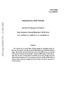
FIG. 1: (Color online.) (a) Three-loop braiding process. The loops A, B and C are colored blue, red and green respectively. The braiding path of loop-C is indicated by the dotted arrow curve. (b) Two-loop linking in the (2 + 1)d space-time, which B corresponds to creating a pair of ZA 2 and Z2 visons, and anniA hilating them after braiding one Z2 and one ZB 2 visons. The time τ is along the vertical direction. The inset shows the local cylindrical coordinate system around a segment of the ZA 2 vison loop.

coupling the SPT phases to a discrete gauge theory can also be described and calculated using this NLSM field theory. Basically the braiding phase factor comes from the Θ−term in the field theory, as long as we carefully analyze the field configuration in the space-time which corresponds to the braiding process. The NLSM field theory with a topological term can be viewed as the continuum limit field theory description for these braiding statistics. 2d Anyon statistics — We will first look at 2d systems, and as an example let B us start with the 2d SPT state with ZA 2 × Z2 symmetry, which can be described by the following (2 + 1)d O(4) NLSM with a Θ-term at Θ = 2π [15]: Z 1 iΘ S = d2 xdτ (∂µ n)2 + abcd na ∂x nb ∂y nc ∂τ nd , (1) g Ω3 where n is a four component vector with unit length, and Ω3 = 2π 2 is the volume of a three dimensional sphere B with unit radius. Under the ZA 2 × Z2 symmetry, the vector n transforms as 1 2 1 2 3 4 3 4 ZA 2 : n , n → −n , −n , n , n → n , n ; 1 2 1 2 3 4 3 4 ZB 2 : n , n → n , n , n , n → −n , −n .

(2)

B Now let us couple the vector n to a ZA 2 × Z2 gauge field. The excitations that will have nontrivial braiding statistics are the vison excitations (π-gauge flux) of gauge fields

2 B ZA 2 and Z2 . Let us consider the following braiding proB cess: one pair of ZA 2 visons and one pair of Z2 visons are created in space at one instance in time, then they are annihilated at another later instance after braiding one ZA 2 vison with one ZB 2 vison. In the (2 + 1)d space-time, this B process corresponds to one linking between ZA 2 and Z2 vison loops, as shown in Fig. 1(b). Because the Z2 gauge fields are coupled to the four-component vector n, the 1 2 ZA 2 vison is bound with a ±1/2-vortex of (n , n ), while B 3 4 Z2 vison is bound with a ±1/2-vortex of (n , n ). Then the braiding process in the space-time can be viewed as a linking configuration between (n1 , n2 ) half-vortex loop and (n3 , n4 ) half-vortex loop. Due to the Θ-term in Eq. (1), this configuration will contribute a phase factor exp(±iπ/2) = ±i to the action, which implies the mutual B braiding statistics between the ZA 2 vison and Z2 vison. To calculate this phase factor explicitly, let us first consider a finite segment of ZA ˆ direc2 vison loop along the τ tion. A vison is always bound with either 1/2-vortex or −1/2-vortex of (n1 , n2 ). Around this segment, the O(4) vector n has the following configuration with cylindrical coordinate (r, φ, τ ) (x = r cos φ, y = r sin φ, see Fig. 1(b) inset):

n1 = sin α(r) cos f (φ), n2 = sin α(r) sin f (φ),

(3)

n3 = cos α(r)N 1 (τ ),

to the action. In other words, the linking configuration in Fig. 1(b) corresponds to ±1/4-instanton of the four component vector n in the (2 + 1)d space-time. Now let us consider a 2d SPT state with Z2 global symmetry only, and couple it to a Z2 gauge field. This SPT state can be described by the same field theory Eq. (1), and under the Z2 symmetry n → −n. A vison of this Z2 gauge field can be viewed as a bound state between B the ZA 2 vison and Z2 vison discussed previously. Then the linking configuration in Fig. 1(b) can be interpreted as creating a pair of visons, self-twisting one vison by 2π, then annihilating them. The phase ±i corresponds to topological spin-±1/4 of the vison, which is consistent with the semion and anti-semion statistics of the vison proved in Ref. 7. All the analysis above can be straightforwardly generalized to ZN gauge theory coupled to a 2d ZN SPT state. The 2d ZN SPT state is described by the same field theory Eq. (1) [15], where Θ = 2πk, k = 0, 1, · · · (N −1). The same analysis above leads to the result that the topological spin of the 2π/N flux excitations can be k/N 2 , namely self-twisting such excitation will grant its wave function a phase exp(2πik/N 2 ). 3d loop statistics — B Now we consider 3d bosonic SPT states with ZA 2 ×Z2 × C Z2 symmetry. In terms of field theory, one of these SPT states is described by the following (3 + 1)d O(5) NLSM:

n4 = cos α(r)N 2 (τ ),

Z 2

where N = (N1 , N2 ) is an O(2) unit vector |N | = 1. N is a function of τ only. α(r) is a nonnegative continuous function that satisfies α(0) = 0, α(∞) = π/2. Along the τˆ axis, i.e. r = 0, we have (n3 , n4 ) = N . Using this configuration, we can compute the Θ-term: Z 2πi abcd na ∂x nb ∂y nc ∂τ nd d2 xdτ Ω3 (4) Z 2π Z i ab N a ∂τ N b . = dφ ∂φ f dτ 2π 0 If n1 and n2 form a full vortex line along the τˆ axis, namely f (φ) ∼ φ, the O(4) Θ-term reduces to a 1d O(2) NLSM with Θ = 2π. If there is a ZA 2 vison line along the τˆ axis, i.e. n1 and n2 form a ±1/2-vortex line along τˆ axis, namely f (φ) ∼ ±φ/2, then the (2 + 1)d O(4) NLSM reduces to a 1d O(2) NLSM of vector N with Θ = ±π. Now let us consider two linked vison loops, and in Eq. (4) τ becomes the parameter along the ZA 2 vison loop. Since the two loops are linked, vector N will have a ±1/2-vortex winding along ZA 2 vison loop: I dτ ab N a ∂τ N b = ±π. (5) Combining Eq. (4) and Eq. (5) together, we conclude that this linking configuration (which corresponds to a braiding process in the space-time) would contribute factor ±i

S=

d3 xdτ

iΘ 1 (∂µ n)2 + abcde na ∂x nb ∂y nc ∂z nd ∂τ ne ,(6) g Ω4

where Ω4 = 8π 2 /3 is the volume of a four dimensional B C sphere with unit radius. Under the ZA 2 × Z2 × Z2 symmetry, the five component vector n transforms as 1 2 1 2 ZA 2 : n , n → −n , −n ,

n3,4,5 → n3,4,5 ;

2 3 2 3 ZB 2 : n , n → −n , −n ,

n1,4,5 → n1,4,5 ;

4 5 4 5 ZC 2 : n , n → −n , −n ,

n1,2,3 → n1,2,3 .

(7)

B C Now let us couple this SPT state to ZA 2 × Z2 × Z2 gauge field, and consider the statistics between the three loops in Fig. 1(a), in which the base loop is a vison loop of ZA 2 gauge field, and it is linked with vison loops of both ZB 2 and ZC 2 gauge fields. A vison loop can be bound with either a +1/2-vortex or −1/2-vortex, both cases exist in the system, and they correspond to different excitations. As an example let us study the braiding statistics of vison loops bound with +1/2-vortex. The choice of +1/2 vortex gives each vison loop an orientation, as marked out in Fig. 1(a). Let us first look at the ZB 2 vison loop. Following the same calculation as Eq. (4), because ZB 2 vison loop is bound with a half-vortex loop of (n2 , n3 ), the O(5) NLSM with Θ = 2π is reduced to an O(3) NLSM with Θ = π in the (1 + 1)d world-sheet of the ZB 2 vison loop, and the three

3 statistics can be described by the NLSM as well. As the vison link braid through the vison loop, the space-time configuration of the O(5) vector n around the vison link can be described as following: n1 = cos α(τ ), n2 = sin α(τ )N 1 (x, y, z), n3 = sin α(τ )N 2 (x, y, z), 4

(9)

3

n = sin α(τ )N (x, y, z), n5 = sin α(τ )N 4 (x, y, z), FIG. 2: (Color online.) The space-time configuration of N ∼ (n1 , n4 , n5 ) on the world sheet of the ZB 2 vison loop (in red) as the ZC 2 vison loop (in green) braiding around it. Each red line is a time slice, at which moment the corresponding three-loop configuration is shown below.

component vector on this world sheet is N ∼ (n1 , n4 , n5 ): Z 1 iπ S1d,B = dxdτ (∂µ N )2 + abc N a ∂x N b ∂τ N c . (8) g 4π On the (1 + 1)d world sheet of ZB 2 vison loop, the braidC ing between ZB 2 and Z2 vison loops corresponds to the space-time configuration N (x, τ ) in Fig. 2, and this configuration carries 1/2 O(3) instanton number, thus it will contribute a factor i to the action. This implies that the three-loop braiding statistics angle is θBC,A = π/2. The statistics angle θAC,B can be calculated in the same way after interchanging n1 and n3 in the O(5) vector, which will lead to factor −1 due to the antisymmetrization in the Θ-term in Eq. (6). Thus θAC,B = −π/2. HbL

HaL A C

ΘB C,A B

HcL B

C

C

A

A

ΘA C,B

B

ΘA B,C

FIG. 3: (Color online.) (a) Braiding a link of the ZB 2 and A ZC 2 vison loops with the Z2 vison loop also accumulates the phase θBC,A . (b,c) The three-loop braiding process that corresponds to the statistic angle θAC,B (θAB,C ). The light blue torus indicates the surface traced out by the ZA 2 vison loop through the braiding processes, which can be considered as the Gaussian surface that measures the ZA 2 charge enclosed. Small arrows on the loops mark out the loop orientation.

The loop braiding statistics can also be understood in a different way. Ref. 16 pointed out that the threeloop braiding in Fig. 1(a) can also be viewed as a link of C A the ZB 2 and Z2 vison loops braiding with the Z2 vison loop, as illustrated in Fig. 3(a). This link-loop braiding

where N = (N 1 , N 2 , N 3 , N 4 ) is an O(4) unit vector |N |2 = 1 that describes the configuration of the (linked) half-vortex loops bound to the vison loops of ZB 2 and ZC . The time τ (running from 0 to 1) parameterizes a 2 C A full braiding of the ZB × Z vison link with the Z vison 2 2 2 loop. Suppose the n1 component is energetically more favored, then the ZA 2 branch cut disk bordered by the ZA vison loop will be bound with a n1 domain wall. Let 2 B the braiding of the Z2 × ZC 2 vison link initiates from one side of the domain wall, and ends up at the other side of the domain wall, then α(τ ) will be a continuous function satisfying α(0) = π, α(1) = 0. Plugging the configuration Eq. (9) into the NLSM Eq. (6), the O(5) Θ-term of n is reduced to an O(4) Θ-term of N at Θ = 2π: Z −

3

dτ ∂τ α sin α Z0

=

1

d3 x

Z

d3 x

2πi abcd N a ∂x N b ∂y N c ∂z N d Ω4

2πi abcd N a ∂x N b ∂y N c ∂z N d . Ω3

(10)

According to our previous calculation, the linking configuration between (N1 , N2 ) half-vortex loop and (N3 , N4 ) half-vortex loop corresponds to the 1/4 O(4) soliton in the 3d space, so the above O(4) Θ-term in Eq. (10) will result in a π/2 phase angle accumulated in the link-loop braiding, which equals to the three-loop braiding angle θBC,A calculated already in our paper. The non-trivial link-loop braiding statistics implies C that the ZB 2 × Z2 vison link must carry the charge of A the Z2 gauge field. Let us denote the ZA 2 charge carC A . It is related ried by the ZB × Z vison link as q 2 2 BC A to the braiding angle by θBC,A = −πqBC . The minus sign is due to the reversed link-loop braiding direction as shown in Fig. 3(a) (which corresponds to the positive three-loop braiding direction). As shown in Fig. 3(b), the torus traced out by the ZA 2 vison loop through braiding with the ZC vison loop (in the linking with the ZB 2 vison 2 loop) actually forms a Gaussian surface enclosing the ZC 2 vison loop. So the three-loop braiding statistics angle C θAC,B measures the ZA 2 charge carried by the Z2 vison C A A B . loop in the Z2 × Z2 link, denoted qC , and θAC,B = πqC Similarly from Fig. 3(c), the three-loop braiding statistics B angle θAB,C measures the ZA 2 charge carried by the Z2 B C A vison loop in the same Z2 × Z2 link, denoted qB , and

4 A A A A θAB,C = πqB . Obviously, qBC = qB + qC , thus

θAB,C + θBC,A + θAC,B = 0,

vector n transforms as (11)

which is precisely the cyclic relation [8, 16], and it implies that θAB,C = 0 (given θBC,A = π/2 and θAC,B = −π/2 as previously calculated). B C A

B

®

ZA 2 : n1 , n2 → −n1 , −n2 , ZB 2 : n1 → n1 ,

n3,4,5 → n3,4,5 ;

n2,3,4,5 → −n2,3,4,5 .

Now a ZB 2 vison loop corresponds to a bound state beB tween the ZC 2 and Z2 vison loops in the previous case. Thus [19] θBB,A = 2θBC,A = π, θAB,B = θAC,B + θAB,C = ±π/2.

C A

FIG. 4: (Color online.) Illustration of moving ZB 2 vison loop A through the ZA 2 vison loop. The Z2 vison loop borders a C branch cut disk, which can be viewed as a 2d ZB 2 × Z2 SPT. B When the Z2 vison loop pokes through this disk, a pair of C ZB 2 semion-antisemion are created, braided with the Z2 vison, and annihilated.

θAB,C can also be computed as follows: θAB,C correB sponds to braiding ZA 2 and Z2 vison loops, both of which C are linked to a Z2 vison loop. This process can be divided A into two steps: first moving ZB 2 vison loop through Z2 A B vison loop, then moving Z2 vison loop through Z2 vison loop. The first step (see Fig. 4) is equivalent to creating a pair of ZB 2 vison-antivison (vison and antivison have C semion and antisemion statistics) at the 2d ZB 2 ×Z2 SPT B phase, then braiding the Z2 vison (or antivison) around the ZC 2 vison, and annihilating the vison-antivison pair. This step will contribute a phase factor i to the action. The second step is equivalent to creating and annihilatA C ing a pair of ZA 2 visons at the 2d Z2 ×Z2 SPT phase, and C braiding around the Z2 vison in between, which will contribute factor −i. The two processes together will lead to a trivial phase factor, namely θAB,C = 0. More “conventionally”, θBC,A and θAC,B can be interpreted in the “decorated domain wall” picture [17]. In our NLSM Eq. (6), the ZA 2 vison loop is the boundary of a 2d disk of branch cut of coupling between n1 components. According to Ref. 18, after integrating out n1 , the effective field theory on this 2d disk is the same as Eq. (1) with Θ = 2π, except now the O(4) vector is (n2 , n3 , n4 , n5 ), i.e. this 2d disk can be viewed as a 2d SPT state with C ZB 2 × Z2 symmetry, which is precisely the decorated doC main wall picture. Then after gauging the ZB 2 and Z2 symmetry, the vison loop statistics reduces to the anyon C statistics of the 2d ZB 2 × Z2 topological order, which is what we have already computed using Eq. (1). B We can also consider 3d SPT state with ZA 2 × Z2 symmetry. There are in total three different nontrivial 3d bosonic SPT states with this symmetry [3]. The first state can be constructed using the previously discussed B C B C ZA 2 ×Z2 ×Z2 SPT state, and break its subgroup Z2 ×Z2 down to one diagonal Z2 symmetry, namely now the O(5)

(12)

(13)

All the other braiding angles are zero. The second type of 3d SPT state corresponds to interchanging ZA 2 and ZB 2 symmetries, thus after gauging the symmetries, θAB,A = ±π/2, θAA,B = π. The third type of SPT state is equivalent to the two SPT states discussed above weakly coupled together, thus θAB,A = θAB,B = ±π/2, θAA,B = θBB,A = π.

(14)

In summary, we have computed the anyon braiding statistics, and three-loop statistics of 2d and 3d topological phases constructed by coupling plain gauge theories to bosonic SPT states. Our calculation is based on semiclassical field theories, and all the braiding phases naturally come from the topological Θ−term in the field theory. We acknowledge the enlightening discussion with Chao-Ming Jian and Meng Cheng. The authors are supported by the the David and Lucile Packard Foundation and NSF Grant No. DMR-1151208.

[1] A. M. Polyakov, Gauge Fields and Strings (Harwood Academic Publishers, 1987). [2] A. Y. Kitaev, Ann. Phys. 303, 1 (2003). [3] X. Chen, Z.-C. Gu, Z.-X. Liu, and X.-G. Wen, Phys. Rev. B 87, 155114 (2013). [4] X. Chen, Z.-C. Gu, Z.-X. Liu, and X.-G. Wen, Science 338, 1604 (2012). [5] D. A. Ivanov, Phys. Rev. Lett. 86, 268 (2001). [6] A. Y. Kitaev, Ann. Phys. 321, 2 (2006). [7] M. Levin and Z.-C. Gu, Phys. Rev. B 86, 115109 (2012). [8] C. Wang and M. Levin, arXiv:1403.7437 (2014). [9] H. Moradi and X.-G. Wen, arXiv:1404.4618 (2014). [10] J. Wang and X.-G. Wen, arXiv:1404.7854 (2014). [11] S. Jiang, A. Mesaros, and Y. Ran, arXiv:1404.1062 (2014). [12] A. Vishwanath and T. Senthil, Phys. Rev. X 3, 011016 (2013). [13] C. Xu, Phys. Rev. B 87, 144421 (2013). [14] C. Xu and T. Senthil, Phys. Rev. B 87, 174412 (2013). [15] Z. Bi, A. Rasmussen, and C. Xu, arXiv:1309.0515 (2013). [16] C.-M. Jian and X.-L. Qi, arXiv:1405.6688 (2014). [17] X. Chen, Y.-M. Lu, and A. Vishwanath, Nature Communications 5, 3507 (2014). [18] Z. Bi, A. Rasmussen, and C. Xu, Phys. Rev. B 89, 184424 (2014).

5 [19] Here θBB,A stands for the full braiding statistics angle between two ZB 2 vison loops while they are both linked

with a ZA 2 vison loop.