Anyonic quantum spin chains: Spin-1 generalizations and topological

Anyonic quantum spin chains: Spin-1 generalizations and topological stability C. Gils,1, 2 E. Ardonne,3, 4 S. Trebst,5, 6 D.A. Huse,7 A.W.W. Ludwig,8 M. Troyer,1 and Z. Wang6 1 Theoretische Physik, Eidgenössische Technische Hochschule Zürich, 8093 Zürich, Switzerland Department of Mathematics and Statistics, University of Saskatchewan, Saskatoon S7N 5E6, Canada 3 Nordita, Royal Institute of Technology and Stockholm University, Roslagstullsbacken 23, SE-106 91 Stockholm, Sweden 4 Department of Physics, Stockholm University, AlbaNova University Center, SE-106 91 Stockholm, Sweden 5 Institute for Theoretical Physics, University of Cologne, 50937 Cologne, Germany 6 Microsoft Research, Station Q, University of California, Santa Barbara, CA 93106, USA 7 Physics Department, Princeton University, Princeton, NJ 08544, USA 8 Physics Department, University of California, Santa Barbara, CA 93106, USA (Dated: March 19, 2013)

arXiv:1303.4290v1 [cond-mat.str-el] 18 Mar 2013

2

There are many interesting parallels between systems of interacting non-Abelian anyons and quantum magnetism, occuring in ordinary SU(2) quantum magnets. Here we consider theories of so-called su(2)k anyons, well-known deformations of SU(2), in which only the first k + 1 angular momenta of SU(2) occur. In this manuscript, we discuss in particular anyonic generalizations of ordinary SU(2) spin chains with an emphasis on anyonic spin S = 1 chains. We find that the overall phase diagrams for these anyonic spin-1 chains closely mirror the phase diagram of the ordinary bilinear-biquadratic spin-1 chain including anyonic generalizations of the Haldane phase, the AKLT construction, and supersymmetric quantum critical points. A novel feature of the anyonic spin-1 chains is an additional topological symmetry that protects the gapless phases. Distinctions further arise in the form of an even/odd effect in the deformation parameter k when considering su(2)k anyonic theories with k ≥ 5, as well as for the special case of the su(2)4 theory for which the spin-1 representation plays a special role. We also address anyonic generalizations of spin-1/2 chains with a focus on the topological protection provided for their gapless ground states. Finally, we put our results into context of earlier generalizations of SU(2) quantum spin chains, in particular so-called (fused) Temperley-Lieb chains. PACS numbers: 05.30.Pr, 03.65.Vf, 03.67.Lx

Contents

I. Introduction

2

II. The anyonic quantum spin chain Hamiltonians A. Topological symmetry

3 5

III. Anyonic su(2)k spin-1 chains: odd k ≥ 5 A. Introduction B. The ordinary SU(2) Heisenberg spin-1 chain C. Phase diagram of the anyonic spin-1 chains – overview D. Critical phases 1. Zk -parafermion phase 2. Z2 -phase: (A, D) modular invariant of coset su(2)k−1 × su(2)1 /su(2)k 3. Z3 -phase: coset su(2)k−4 × su(2)4 /su(2)k 4. Superconformal critical point 5. Stability of the critical phases E. The gapped Haldane phase 1. Energy spectrum 2. Phase boundaries 3. Ground states in the periodic chain (anyonic equivalent of AKLT point) 4. Ground states in the open chain (anyonic equivalent of AKLT point)

6 6 6

IV. Anyonic su(2)k spin-1 chains: even k ≥ 6 V. Anyonic su(2)k spin-1 chains: k = 4 A. Hilbert space and Hamiltonian

7 8 8

B. Phase diagram in the integer Hilbert space sector (IS) 1. Gapped phases (IS) 2. Gapless phases (IS) C. Phase diagram in the half-integer Hilbert space sector (HIS) 1. Gapped phases (HIS) 2. Gapless phases (HIS) D. The location of the phase boundaries VI. Anyonic su(2)k spin-1/2 chains A. The ferromagnetic case B. The anti-ferromagnetic case VII. Discussion

11 11 11 11 12 12 12 12 13 14 16 16

Acknowledgments

16 16 17 19 19 20 20 22 24 24 25 27

A. su(2)k anyons

27

B. F -matrices of the su(2)k theories

29

C. Microscopic models 1. Basis and Hamiltonian 2. Hamiltonian of the su(2)k spin-1/2 chain a. su(2)2 spin-1/2 chain b. su(2)3 spin-1/2 chain c. su(2)4 spin-1/2 chain d. su(2)5 spin-1/2 chain 3. Hamiltonian of the su(2)k spin-1 chain a. The su(2)4 spin-1 chain

30 30 30 31 31 31 31 31 32

2 b. The su(2)5 spin-1 chain c. The su(2)6 spin-1 chain d. The su(2)7 spin-1 chain

32 32 33

scribed as theory of ordinary SU(2) quantum spins that is deformed in such a way that only the first k + 1 (generalized) angular momenta

D. Exact form of the AKLT states

34

k 1 j = 0, , 1, . . . , 2 2

E. Conformal field theories of interest 1. Virasoro minimal models 2. N = 1 superconformal minimal models 3. S3 minimal models 4. The Zk parafermion CFT. 5. The Z2 orbifold theories a. The S-matrix

34 34 35 35 35 35 35

References

36

I.

INTRODUCTION

Ever since the early days of condensed matter physics, quantum magnets have played an integral role in shaping our understanding of interacting quantum many-body systems. Following the experimental discovery of the high-temperature superconductors whose undoped parent compounds typically are antiferromagnets, the study of quantum magnets has further intensified yielding a plethora of deeper insights. Early on, quantum spin chains – typically one-dimensional arrangements of SU(2) spins – have become prototypical systems that proved to be fruitful ground for analytical descriptions and quasi-exact numerical analysis1 . One seminal result was the exact solution of the antiferromagnetic spin-1/2 Heisenberg chain via the Bethe ansatz and its description in terms of conformal field theory. Another crucial contribution was Haldane’s realization2 that the antiferromagnetic spin-1 Heisenberg chain forms a gapped state with characteristic zeroenergy edge states for open boundary conditions – a principle observation that holds true for all half-integer and integer spin chains. More recently, it has been found that the gapped Haldane phase of the spin-1 chain is an example of a symmetry protected topological phase3,4 making it a onedimensional cousin of topological insulator states in two and three dimensions5 , which have attracted much recent interest. Over the years, a plethora of physical systems that connect to the elementary physics of quantum spin chains have been identified, including transition metal oxides6 , Au quantum wires on semiconducting surfaces7 , or ultra-cold atoms in optical lattices8 . Recently, it has been realized that certain ‘deformations’ of quantum spins can be used to describe some of the more peculiar topological properties of exotic quasiparticles, so-called non-Abelian anyons, that arise in certain topologically ordered systems, including certain fractional quantum Hall states9 , px + ipy superconductors10 , heterostructures of topological insulators and superconductors11 , heterostructures of spin-orbit coupled semiconductors and superconductors12 and possibly certain Iridates13 which may effectively realize the Kitaev honeycomb model14 . To be more specific, the deformations of quantum spins are representations of the anyon theories called su(2)k , which can be de-

can occur. These generalized angular momenta capture the non-Abelian properties of the anyonic quasiparticles present in the su(2)k theory. For instance, the non-Abelian nature of the so-called Majorana fermion is captured by the generalized angular momentum 1/2 of the su(2)2 theory. The same holds for so-called Ising anyons, while Fibonacci anyons can be represented by the generalized angular momentum 1 of the su(2)3 theory. Similar to the coupling of two ordinary spins, a pair of generalized angular momenta can be combined (or ‘fused’) into a new set of joint quantum numbers. For instance, for k ≥ 2, two generalized angular momenta 1/2 can be combined to form either a state with generalized angular momentum 0 or a state with generalized angular momentum 1, which is written as 1/2 × 1/2 = 0 + 1 ,

(1)

reminiscent of two ordinary spin 1/2’s forming either a singlet or triplet state. Similarly, two generalized angular momenta 1 can be combined into 1×1=0+1+2

(2)

for deformation parameters k ≥ 4. For lower values of k, the rules differ because the number of representations is limited by k. In particular, for k = 3, one finds 1 × 1 = 0 + 1, while for k = 2, one has 1 × 1 = 0. Finally, for k = 1, the general momentum 1 is not allowed. For the anyonic theories, the above equations are often referred to as fusion rules. The many-body physics of a set of interacting non-Abelian anyons can be captured by a Hamiltonian that is formed by pairwise interactions which assign energies to the different outcomes in the above fusion rules. Such an approach is a straightforward generalization of the conventional Heisenberg ~i · S ~j is simply a model, whose pairwise interaction term J S projector onto the singlet state, which is energetically favored for antiferromagnetic couplings (J < 0) or penalized for ferromagnetic couplings (J > 0). The first step in this direction was taken by some of us for anyonic spin-1/2 chains in Ref. (16) and later generalized to spin-1 chains in Ref. (17) by the current group of authors. The careful analysis of the ground states of these one-dimensional systems has resulted in a number of insights. First, anyonic spin-1/2 chains typically form gapless ground states which can be described in terms of conformal field theory16 . These gapless states turn out to be protected by a topological symmetry inherent to the anyon chains that renders them stable against local perturbations16,18 . Moreover, these gapless states can in fact be interpreted as edge states that reveal the true ground state of a two-dimensional set of anyons – a novel topological liquid that is separated by the original topological liquids (of which the anyons are excitations) by an edge17 .

3 This picture has been verified by a careful analysis of ladder systems, in which multiple chains are coupled19 . Going beyond spin-1/2 chains, we began to study the physics of anyonic spin-1 chains with first results being reported in a preceding (much more condensed) paper17 . In the manuscript at hand, we provide an in-depth discussion of these anyonic spin-1 chains. We find that many of the distinctive features of ordinary SU(2) spin-1/2 and spin-1 chains also hold for their anyonic cousins. For instance, anyonic spin-1 chains exhibit a gapped topological phase for antiferromagnetic couplings – the anyonic generalization of the Haldane phase. Exploring the phase diagram of chains of pairwise interacting spin-1 anyons, we find a striking resemblance of the anyonic phase diagram to the one of the ordinary bilinearbiquadratic spin-1 chain. In particular, we find multiple gapless phases (and phase transitions) in addition to the gapped Haldane phase. For the former, a similar topological protection mechanism and edge state interpretation holds as for the gapless phases of the anyonic spin-1/2 chains17 . The focus of this manuscript is to provide an exhaustive description of the phase diagram(s) of the anyonic spin-1 chains. Our exploration of these systems has led to a large amount of results as the phase diagrams turned out to be much richer than initially anticipated. In particular, we find two families of phase diagrams depending on whether the deformation parameter k of the su(2)k anyonic theories is odd or even. Moreover, we obtain a distinct phase diagram for k = 4, a result that can be explained by the special role played by the generalized angular momentum 1 in the su(2)4 theory. In order to guide the reader through these various results we have taken some care to structure the manuscript as follows: We will start with an introduction to the anyonic su(2)k theories and a description of the anyonic generalization of the Heisenberg model in Section II. The following sections will then give a detailed exposé of our results, devoting Sec. III to the discussion of anyonic spin-1 chains with odd deformation parameters k ≥ 5, followed by a discussion of the case of even deformation parameters k ≥ 6 in Sec. IV. In Sec. V we will turn to the case of k = 4 for which the spin-1 representation plays a special role and a rich phase diagram is obtained. We will then turn to anyonic spin-1/2 chains and discuss their physics, in particular their topological stability in Sec. VI. We will end with a broader discussion of our results, in particular in light of other deformations of conventional spin chains such as continuous su(2)q deformations or so-called (fused) Temperley-Lieb spin chains. The main part of the manuscript is followed by an appendix that provides the technical details of our calculations.

II.

THE ANYONIC QUANTUM SPIN CHAIN HAMILTONIANS

In light of the recent interest in topological phases of matter, it is of great importance to gain an understanding topological models in their simplest incarnation, and we will thus study one-dimensional chains of interacting non-Abelian anyons. In this section, we will briefly explain the models by drawing

parallels with ordinary one-dimensional spin chains. Moreover, we will explain why the ‘topological’ nature of these models goes beyond the fact that they are constructed from ‘topological’ particles, namely non-Abelian anyons. One of the prototypical one-dimensional spin chain models is the Heisenberg model, in which SU(2) spins interact via a ~i · S ~j , where the labels i ‘spin-spin’ interaction of the type S and j denote the locations of the interacting spins. Often, one restricts the interaction to nearest-neighbor, or next-nearestneighbor pairs of spins. For the description of the anyonic quantum spin chains, it will be beneficial to think of this interaction in terms of the total spin of the two interacting spins. In this paper, we will only consider nearest neighbor interactions. As a first example, we look at conventional SU(2) spin-1/2, ~T = (S ~ i +S ~i+1 ) of two interacting and consider the total spin S ~ ~ spins Si and Si+1 , whose magnitude is characterized by the ~T )2 = (S ~i + S ~i+1 )2 . Because the total spin eigenvalue of (S ~T can be either 0 or 1, with S ~ 2 eigenvalues 0 and 2, we can S T write (0)

~i + S ~i+1 )2 = 0P (S i

(1)

+ 2Pi

,

(3)

(s)

where the projection operator Pi projects onto the total spin ~i and S ~i+1 . Evaluating the left s channel of the two spins S hand side, one obtains ~i · S ~i+1 = P (1) − 3 Ii = −P (0) + 1 Ii , S i i 4 4

(4)

where in the last step we used that we can rewrite the iden(0) (1) tity operator as Ii = Pi + Pi , which holds in the case of spin-1/2. We conclude that the Heisenberg interaction assigns energy to two interacting spins, depending on their combined spin, and the Heisenberg Hamiltonian can be written in terms of projectors as X (0) H=J Pi , (5) i

where J = 1 corresponds to an antiferromagnetic coupling, and J = −1 to the ferromagnetic version. For spin-1, one can similarly write the bilinear and bi~i · S ~i+1 and (S ~i · S ~i+1 )2 respectively, in terms quadratic terms S (1) (2) of the projection operators Pi and Pi . In particular, the relations (1)

~i + S ~i+1 )2 = 2P (S i

(2)

+ 6Pi

~i + S ~i+1 )4 = 4P (1) + 36P (2) , (S i i

(6)

can be rewritten as ~i · S ~i+1 ) = P (1) + 3P (2) − 2Ii (S i i

~i · S ~i+1 )2 = −3P (1) − 3P (2) + 4Ii . (S i i

(7)

Consequently, the bilinear-biquadratic spin-1 Hamiltonian X ~i · S ~i+1 ) + sin(θbb )(S ~i · S ~i+1 )2 (8) Hbb = cos(θbb )(S i

4 (1)

can be expressed in terms of the projectors Pi follows, X (2) (1) Hbb = J 2 Pi + J 1 Pi

(2)

and Pi

as

i

=

X

(2)

cos θ2,1 Pi

i

(1)

− sin θ2,1 Pi

.

(9)

Here, the relation between the two angles θ2,1 and θbb is given by tan θ2,1 =

tan θbb − 1/3 1 − tan θbb

tan θbb =

tan θ2,1 + 1/3 . 1 + tan θ2,1 (10)

We will now shift our attention to anyonic degrees of freedom. Details about anyon models, in particular those of type su(2)k , can be found in appendix A. A general introduction can be found, e.g., in references Ref. (14,15,20). Here, we will only introduce those concepts that are necessary for defining the chain Hamiltonians. The Hamiltonians for the anyon chains that we will consider in this paper are of the form of (j) Eq. (9). The projectors Pi in that equation have however a different meaning for anyons (as compared to ordinary spins) which will be defined in Eq. (12) below. Anyons are labeled by generalized angular momenta, or - in the language of anyons models - ‘topological charges’. These generalized angular momenta correspond to quantum numbers, just as in the case of ordinary spin degrees of freedom. The notion of combined spin, or tensor product of spins, corresponds to the notion of ‘fusion’ in the language of anyons, and can in general result in more than one type of anyon. The possible outcomes are called ‘fusion channels’. The generalization of the Heisenberg interaction for spins to the anyonic case is to assign an energy to two interacting anyons based on their fusion channel. How this is done in practice, will be described in more detail below and in appendix C. The class of anyons considered in this paper is derived from SU(2) where spin-S ranges from S = 0, 1/2, 1, 3/2, . . .. In contrast, su(2)k anyons contain only a subset of generalized angular momenta, namely 1 k j = 0, , 1, . . . , . 2 2 The truncation, characterized by the ‘level’ k, has two important consequences which we will describe in the following. The first consequence concerns the fusion rules of the anyons. The tensor product of two SU(2) spins S1 and S2 decomposes as S1 ⊗ S2 = |S1 − S2 | ⊕ · · · ⊕ (S1 + S2 ) . The process of taking tensor products is associative, and the same is true for the fusion rules. Because of the truncation in the su(2)k theory, the SU(2) tensor product rule has to be modified. It turns out that there is only one way of doing this, consistent with the requirement that the fusion rules are

associative. In particular, the fusion rules of su(2)k anyons read j1 ×j2 = |j1 −j2 |+(|j1 −j2 |+1)+· · ·+min(j1 +j2 , k−j1 −j2 ). (11) The second important consequence of the truncation follows from the fusion rules. The dimension of the Hilbert space of a number N of ordinary SU(2) spin-1/2’s is equal to 2N , and the spins can add up to a maximum spin of N/2. In contrast, the dimension of the Hilbert space of a number N of j = 1/2 anyons in the su(2)k theory is smaller than 2N . In appendix A, it is shown that the dimension of the Hilbert space for N j = 1/2 anyons grows as dN , asymptotically for 1/2 π large N , where d1/2 = 2 cos k+2 is the so-called quantum dimension of the j = 1/2 anyon. For 1 < k < ∞, this implies that the effective number of degrees of freedom for each anyon is irrational. This is less mysterious than it sounds: all this is saying is that one can not think of the Hilbert space of N anyons as a tensor product of N one-anyon Hilbert spaces. Because the Hilbert space does not have a tensor product structure, an alternative description of the state space and the Hamiltonian acting on it is needed. We will describe here how this can be done, but leave the details for the appendices where we also give an explicit description of the Hamiltonians studied in this paper. The Hilbert space of a chain of anyons can be described in terms of a so-called ‘fusion tree’. In Figure 1, the fusion tree for a chain of ‘spin-1’ anyons is displayed. The lines in the fusion tree carry a label indicating the type of anyon the line corresponds to. The lines coming from above correspond to the spin-1 anyons which constitute the chain. The horizontal lines, labeled by xi , are the actual degrees of freedom. The possible ‘values’ of the xi are the same as those of the anyons present in the anyon model, namely xi = 0, 1/2, . . . , k/2, in case of su(2)k anyons. The xi cannot be chosen arbitrarily, but may only take values such that the fusion rules are obeyed at the trivalent points. For example, the anyon type x1 has to appear in the fusion product of x0 × 1, the anyon type x2 appears in the fusion product x1 × 1, and so on. Each labeling of the fusion tree that is consistent with the fusion rules corresponds to a (orthonormal) state in the Hilbert space, and these states span this space. Typically, we will use periodic boundary conditions xL = x0 , which implies that x0 has to appear in the fusion product xL−1 × 1, where L denotes the number of sites of the chain. States in the Hilbert space will be written as |x0 , x1 , . . . , xL−1 i. The Hamiltonian assigns an energy based on the fusion channel of two neighboring anyons in the chain. However,

1 1 1 1 1 x0 x1 x2 x3

...

FIG. 1: The anyonic spin-1 chain.

5

1 1 1 1 1 x0 x1 x2 x3

1 1 1 1 1

F

...

x0

x1

x ˜2 x3

displayed (in this particular case, L = 3). j

j

...

FIG. 2: The basis transformation for the anyonic spin-1 chain.

x1

x0

j

x2

x0 (13)

in the above discussed representation of the Hilbert space (see Figure 1), the fusion channel of two neighboring anyons is not explicit. To remedy this problem, we employ a local basis transformation which changes the order in which the anyons are fused. This is permissible because of the associativity of the fusion rules. For ordinary SU(2) spins, this basis transformation is described in terms of the Wigner 6j-symbols. In the case of anyons, this basis transformation is described by what are known as the F -symbols. A detailed discussion of the F symbols, as well as explicit representations for su(2)k anyons can be found in appendix B. The basis transformation is depicted in Figure 2. On the left hand side, x1 is fused with a spin-1 anyon, resulting in x2 , which is subsequently fused with the next spin-1 anyon, resulting in anyon type x3 . After the basis transformation, one first fuses the two spin-1 anyons, resulting in x ˜2 , which is fused with x1 , resulting in the anyon type x3 . Both bases are equivalent; however, in the second basis, the fusion channel of the two spin-1 anyons is explicit, namely x ˜2 . Thus, after performing this basis transformation, one can assign the appropriate energy based on the value of x ˜2 . Subsequently, one transforms back to the original basis. The operator projecting onto the anyon−j channel of two neighboring anyons i and i + 1 is thus given by (j)

Pi

(j)

= Fi−1 Πi Fi ,

For each type of anyon l, there exists a topological operator Yl . The action of this operator Yl on the state |x0 , x1 , . . . , xL−1 i, displayed in (13) for L = 3, can be described as follows. First, an additional anyon of type l is created inside the spine of the fusion tree, as displayed in (14).

x1

x0

x2

This additional spin-l anyon is ‘merged’ with the fusion dia x00 gram by applying an F -matrix, namely, Flx0 ,x0 ,l , result0 ing in the state X

Flx0 ,x0 ,l

x00

x00 0

|x0 , x1 , . . . , xL−1 i

as depicted in (15). j

j

x1

x0

j

x2

x0

l

x�0

(15)

Next, one ‘moves’ the additional spin-l anyon around the ring, by applying additional F -matrices. After the first step, one obtains the state X

Flx0 ,x0 ,l

x00 ,x01

x00 0

1 ,l Fxj,x 0 0

x01 x0

|x0 , x1 , . . . , xL−1 i

as illustrated in (16). j

x�1 x1

Topological symmetry

j

x2

x0

l

x�0 In this section, we present a detailed discussion of the ‘topological symmetry operator’. The Hamiltonians considered in this paper commute with the topological symmetry operator, and the associated symmetry plays a crucial role in the analysis of the anyonic chain models. In ‘equation’ (13), a chain of type-j anyons with periodic boundary conditions is

x0 (14)

j

A.

j

l

(12)

where Fi is shorthand for the local basis transformation de(j) picted in Figure 2. The operator Πi projects onto the fusion channel x ˜i = j, i.e., the fusion of two anyons into an anyon of type j is penalized with energy E = 1, while the other possible fusion channels are assigned E = 0. For explicit matrix (j) representations of Pi we refer to appendix C. It is important to realize that the form of the projector (12) is universal and applicable to anyonic chains composed of arbitrary types of anyons. Changing to a different anyon model will merely result in a different structure of the Hilbert space and different F -symbols.

j

j

(16)

Another move of this sort gives X

x00 ,x01 ,x02

Flx0 ,x0 ,l

x00 0

1 ,l Fxj,x 0 0

x01 x0

2 ,l Fxj,x 0 1

x02 x1

|x0 , x1 , . . . , xL−1 i

6 as shown in (17). j

j

x�1

j

x�2

x2

x0

l

x�0

(17)

Finally, after L steps, one has come full circle, giving rise to the states X

Flx0 ,x0 ,l

x00 ,x01 ,...,x0L

x00 L−1 Y 0

j,xi+1 ,l

Fx 0

|x0 , x1 , . . . , xL−1 i

xi

i

i=0

x0i+1

as depicted in (18), for L = 3. j

j

x�1

j

x�2 l

x�0

III.

x��0

xi

We can now state the matrix elements of the topological operator Yl in the fusion tree basis

L−1 Y j,x ,l x0i x00 , x01 , . . . , x0L−1 Yl |x0 , x1 , . . . , xL−1 i = Fx0 i i=0

i+1

xi+1

(20) The above definition of the topological operator does not depend on whether the additional spin-l anyon is encircled by the anyon chain (as in Figures (14)-(18)) or whether the additional spin-l anyon encircles the entire anyon chain. When using the latter description of the topological operator, one can think of the additional spin-l anyon as going around the ‘fusion product’ of all the spin-j anyons constituting the anyonic chain, or better, encircling the flux through the chain. This flux through the chain is related to the additional spin-l anyon as follows,

l

i

=

Introduction

(18)

Yl |x0 , x1 , . . . , xL−1 i = L−1 X Y j,x ,l x0i+1 Fx0 i+1 |x0 , x1 , . . . , xL−1 i . (19) i

ANYONIC SU(2)k SPIN-1 CHAINS: ODD k ≥ 5 A.

x0

From the general properties of anyon models (see e.g. Ref. ( 14,15)), we find that x000 = x00 (the overall topological quantum number of an isolated set of anyons can not change). We can now remove the additional spin-l anyon in the same way as we added it, thereby finishing the operation of acting with Yl on the state |x0 , x1 , . . . , xL−1 i. Thus, we obtain the expression

x00 ,x01 ,...,x0L−1 i=0

where i denotes the flux going through the chain, and the matrix S is the modular S-matrix of the anyon model. For a derivation of Eq. (21), see e.g. Ref. (14,15), and the explicit form of S in the case of su(2)k anyons is given in appendix A. The definition of the topological operator contains elements of the F matrices only. This is also true for the anyonic spin Hamiltonians we consider in this paper. It follows that the operators Yl commute with the Hamiltonian and that a topological quantum number can be assigned to all the eigenstates. This has far reaching consequences for the stability of the critical phases. Excited states which are relevant in the renormalization group sense (i.e., have energy smaller than 2) may lie in a different topological sector than the ground state and thus do not drive the system into a different phase. In addition, we will see that the operators Yl play an important role in the zero-energy ground states at the AKLT point in the Haldanegapped phase of the spin-1 models.

Sl,i S0,i i

,

(21)

We will start our discussion of anyonic quantum spin chains with the anyonic version of the ordinary SU(2) spin-1 Heisenberg chain, which has long been appreciated as one of the paradigmatic spin chain models. For antiferromagnetic couplings the spin-1 chain is well known to form a gapped phase, in distinction from the gapless spin-1/2 Heisenberg chain2 . In the following sections, we discuss in detail the anyonic su(2)k deformations of the ordinary SU(2) spin-1 chain. We will see that much of the seminal features of the SU(2) spin-1 chain carry over to these anyonic deformations with a number of new subtleties arising. One is a dependence of the observed phases and phase diagrams on the deformation parameter k. In particular, we find an even/odd effect in k for k ≥ 5 and a distinctive behavior for k = 4. We have therefore split our discussion of the anyonic spin-1 chains into three different sections. We will address anyonic spin-1 chains with odd k ≥ 5 in the remainder of this section, in which we will also give a brief recount of the phase diagram of the ordinary SU(2) . spin-1 chain. The subsequent section will be devoted to the case of k ≥ 6 with k being even. Finally, an entire section is devoted to a detailed account of the physics for the special case of k = 4.

B.

The ordinary SU(2) Heisenberg spin-1 chain

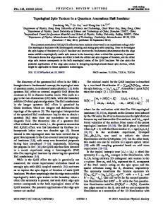
Before addressing the physics of the anyonic spin chains we briefly recapitulate the phase diagram of the ordinary SU(2) spin-1 Heisenberg chain. While the latter is typically discussed as a circle phase diagram in terms of bilinear and biquadratic spin exchange, we will recast the phase diagram in terms of the projector representation in Eq. (9) - the generic representation of anyonic spin chains. Fig. 3 shows the phase diagram in the projector representation of Eq. (9). It contains four different phases, of which two are gapped phases and two

7

su(2)k

SU(2) spin-1 chains

spin-1 chains (odd k)

SU(3) SU(3)

nematic

su(2)k 4 su(2)4 su(2)k

c=2

Haldane ferromagnet

Zk-parafermions

AKLT

dimerized

super CFT (N = 1) su(2)k 2 su(2)2 su(2)k

c = 3/2 SU(3)

are gapless phases. The well known Haldane phase2 extends in the parameter regime − arctan(2/3) < θ2,1 < π/2 and includes the so-called Affleck-Kennedy-Lieb-Tasaki (AKLT) point21 at θ2,1 = 0 (in which only the projector P (2) is present in the Hamiltonian), at which the exact form of the groundstate wave function in terms of a valence bond solid state can be obtained. The conventional (gapped) Heisenberg chain (bilinear in spin-1 operators) with antiferromagnetic coupling corresponds to θ2,1 = − arctan(1/3). The second gapped phase is a (spontaneously) dimerized phase22 that occurs in the parameter regime −π/2 < θ2,1 < − arctan(2/3). The phase transition at θ2,1 = − arctan(2/3) between the two gapped phases is described by the su(2)2 conformal field theory with central charge c = 3/2, which happens to possess N = 1 supersymmetry – a result that can be obtained by means of a (nested) Bethe Ansatz23 . At the other end of the Haldane gapped phase, θ2,1 = π/2, there is a phase transition to gapless phase that extends over the range π/2 < θ2,1 < 3π/4. This critical phase can be described by a conformal field theory with central charge c = 2. There are characteristic quadrupolar (nematic) spin correlations24 in this phase, as well as a three sublattice structure25 resulting in soft modes at momenta K = 0, 2π/3, 4π/3. At the transition from the gapped Haldane phase to this critical nematic phase at θ2,1 = π/2, the system has enhanced SU(3) symmetry. This point in the phase diagram of the spin-1 SU(2) chain represents actually the SU(3) chain with a fundamental representation at each site, which is known to be described by the SU (3)1 conformal field theory. (This chain is again exactly solvable by a Bethe Ansatz26,27 .) Finally, there is a gapless ferromagnetic phase, extending over the parameter range 3π/4 < θ2,1 < 3π/2. The phase transitions from this phase to both the adjacent dimerized phase as well as the nematic phase are first order. In the vicin-

AKLT

su(2)k 1 su(2)1 su(2)k

SU(2)2

FIG. 3: (color online) Phase diagrams of the ordinary SU(2) spin-1 chain in a projector representation (9) with J1 = − sin(θ2,1 ) and J2 = cos(θ2,1 ).

‘Haldane’

FIG. 4: (color online) Phase diagrams of the anyonic su(2)k spin1 chain with odd k in a projector representation (9) where J1 = − sin(θ2,1 ) and J2 = cos(θ2,1 ). With increasing (odd) index k ≥ 5 the phase boundaries move as indicated by the arrows.

ity of the transition between the dimerized and ferromagnetic phase, early analytical work28 suggested the possibility of an intermediate nematic phase, which, however has later been found to not materialize24,29,30 .

C.

Phase diagram of the anyonic spin-1 chains – overview

In this section, we provide an overview of the phase diagram of the anyonic spin-1 chains for odd k ≥ 5. This phase diagram bears great resemblance to the corresponding phase diagram of the SU(2) spin-1 Heisenberg chain (Fig. 3). The generic phase diagram for the su(2)k spin-1 chain is given in Figure 4. In Figures 5 and 6, we display the phase diagrams for k = 5 and k = 7, as well as the characteristic spectra of the four different phases and the (N = 1) super-symmetric critical point which separates the Haldane gapped phase and the phase which will be called “Z2 sublattice phase” (this is the phase intervening between the Haldane phase and the Zk -parafermion phase, and it encompasses the angles θ2,1 . −0.19π ≈ − arctan(2/3)). The spin-1 anyonic spin chain is gapped in a finite region around θ2,1 = 0. This gapped phase is the anyonic analogue of the Haldane gapped phase, and the point θ2,1 = 0 is equivalent to the AKLT point. At this point, the Hamiltonian penalizes the fusion of two neighboring anyons in the spin-2 channel. The ground states with periodic boundary conditions can be found exactly at this point, for all k, and the ground state degeneracy is (k + 1)/2. For θ2,1 < 0, there is a phase transition at θ2,1 ≈ −0.19π into an extended critical region. The position of this phase transition did not show any appreciable dependence on the value of k (remember that k ≥ 5 throughout this section). This gapless region occurs where the ordinary SU(2) spin-1

8 chain is in the gapped dimerized phase. This difference in behavior is the most remarkable distinction between the ordinary SU(2) spin-1 chain, and the anyonic spin-1 chains. The critical point at θ2,1 ≈ −0.19π ≈ − arctan(2/3), separating the Haldane phase and the extended critical region, is described in terms of an N = 1 super-symmetric minimal conformal model. For angles θ2,1 > 0, there is a phase transition from the Haldane phase into another extended critical region which bears some resemblance to the extended nematic region in case of the ordinary spin-1 chain. In particular, this phase has a Z3 sublattice structure. The location of the phase transition does depend on k, and moves towards θ2,1 = π/2 with increasing k. Finally, there is an extended critical region in the vicinitiy of θ2,1 = π, the point where the fusion of two neighboring anyons into the spin-2 channel is favored. This critical phase is the anyonic analogue of the ferromagnetic phase of the ordinary spin-1 chain, and the critical behavior is described by the Zk parafermion conformal field theory. The phase transitions from the ferromagnetic phase to the neighboring extended critical regions are first order. The phase transition into the anyonic version of the nematic phase occurs at θ2,1 = 3π/4, independent of the value of k. The location of the other phase transition depends on k, and moves towards θ2,1 = 3π/2 for increasing k. Below, we will discuss in detail each of the phases mentioned above. We will focus on the topological properties and the similarities to the ordinary SU(2) spin-1 chain.

D.

Critical phases

We investigate the phase diagram of our model numerically using exact diagonalization. In our analysis, we follow a standard procedure to determine the conformal field theory describing the behavior of the extended critical regions and the critical points: the numerically obtained spectrum is first shifted (by some constant offset) such that the ground state has zero energy zero. The spectrum is then rescaled such that the energy of the lowest lying excitation matches the energy of the lowest lying excitation of the conformal field theory describing the phase. The so obtained energy spectrum is finally compared to the energy spectra of candidate CFTs. The CFT (if any) which matches the numerically obtained energy levels is the one describing the system at the angle θ. We note that the list of candidate CFTs is limited: If the chain is critical, each energy level in the spectrum corresponds to a field in the applicable conformal field theory. These fields satisfy fusion rules which have to be compatible with the fusion rules of the underlying su(2)k theory. This constraint restricts the candidate conformal field theories that could describe the criticality of anyonic quantum chains. The eigenenergies in a system of finite size described by a conformal field theory take the form31 E = E1 L +

2πv c ¯ , − +h+h L 12

(22)

where the velocity v is an overall scale factor, and c is the cen¯ take the tral charge of the CFT. The scaling dimensions h + h 0 0 ¯ ¯ form h = h +n, h = h + n ¯ , with n and n ¯ non-negative inte¯ 0 are the holomorphic and antiholomorphic gers, and h0 and h conformal weights of the primary fields in the given CFT. The ¯ + K0 or momenta K (in units 2π/L) are such that K = h − h ¯ + K0 + L/2, where K0 is a constant shift of the K = h−h momentum that determines at which momentum the primary field occurs. This shift can be determined from the numerics, and is not fixed by conformal symmetry. Thus, different microscopic realizations of the same conformal field theories can give rise to different values for K0 . As explained in section II A, the anyonic spin chains have a topological symmetry; all the states in the spectrum can therefore be assigned a topological quantum number. The possible eigenvalues of the topological symmetry operator, also denoted as topological quantum numbers, are in one-to-one correspondence with the types of anyons which appear in the particular anyon theory considered. 1. Zk -parafermion phase

We begin the discussion of the phase diagram given in Figure 4 with the Zk -parafermion phase which corresponds to the gapless ferromagnetic phase in the SU(2) spin-1 chain. In the anyonic spin-1 chains, this phase contains the point θ2,1 = π where it is favorable for two neighboring anyons to be in the spin-2 channel. One of the phase boundaries of this phase is located at θ2,1 = 3π/4. The location of the other phase boundary depends on k: with increasing k, it moves towards the location of the phase boundary in the SU(2) spin-1 chain (at angle θ2,1 = 3π/2). The spectra at angle θ2,1 = π for k = 5 and k = 7 are displayed in the middle panel of Figures 5 and 6, respectively. The energy spectra were rescaled such that the energy of the lowest excitation matches the energy predicted by the Zk parafermion conformal field theory32 . Some details of this CFT are reviewed in appendix E 4. In the Figures, we indicate the locations of the energies of the states corresponding to the primary fields by green squares, while blue crosses correspond the numerically obtained energy levels. We find good agreement between numerically obtained energy spectra and the Zk parafermion CFTs for both the su(2)5 and su(2)7 anyon models. For su(2)5 , we also indicate the location of a few descendant fields that match the numerical prediction. Generally, the identification of descendant fields is more difficult due to finite size effects. The fields of the Zk parafermion theory carry two labels, (l, m) that take the values l = 0, 1, . . . (k − 1), and m = 0, 2, . . . 2(k − 1). The momentum and topological quantum number of the fields is determined by the labels m and l, respectively. The topological quantum number simply is given by l. For the momentum, the following relation holds: K = 2mπ k .

9

su(2)5

spin-1 chain

Z5 sublattice c=8/7

energy E(K)

Z3 sublattice c = 6/7 AKLT

‘Haldane’

0.8

0.8

0.6

0.6

0.4

0.4

Haldane phase

0.2

Z2 sublattice c=6/7

c = 81/70 0

2π

momentum K

3

2 1+4/35 2

8/5 0

0 8/5

2

1

1

1

2 46/35 46/35 2 1+6/35 1+6/35 1

34/35

1+4/35 34/35

1

1

θ/π = 1

1 4/7

Z5 sublattice c = 8/7 2

4/35

1 6/35

6/35 1

0 2π/5

0

4π/5

2

1 8/3 1 2 1+2/7 1 1+2/21 2

1

1 10/7 2 1+2/7 1 1+2/21 2 20/21

0

2 1 0

6π/5

2π

8π/5

momentum K

1 2

1

2

2+2/21 1+20/21

2

1+2/21 20/21

1

θ/π = 3/2

4/35 2

0

0

3

2 1

rescaled energy E(K)

12/7


3π/2

2 2

0

0 π

π/2

0

2

0.2

θ/π = 0 θ/π = 0 θ/π = −0.03 θ/π = +0.03

Z2 sublattice, c = 6/7

2/7 2/21 0

2/21

1

π

π/2

0

momentum K

0 3π/2

2π

3 3

3

3

E(K)

1 2 1 2

16/7

2

2

1

0

9/5

1+3/7

1 1 2

1+8/35

1

1 1 2

1+3/35

73/56

1

269/280

2 0

27/40

0

3/7 1 8/35 1 3/35 2 0 0

0

1 -1

θ/π = -tan (2/3)

rescaled energy


8/3 2+2/7 2

π/2

10/7 1 1+2/7

momentum K

0 3π/2

2π

2

2 1+2/21 20/21

1

1

1

2

θ/π = 0.7 0

Z3 sublattice c = 6/7

2

2/7

2 1

π

2+2/21 1 2 1+20/21

2

superCFT, c = 81/70 9/56 29/280

0

0 0

0

2/21

1

2π/3

momentum K

0 4π/3

2π

FIG. 5: (color online) The su(2)5 spin-1 chain: The energy spectra for the various phases of the phase diagram are shown in the upper left panel. For the critical phases/point the energy spectra have been rescaled to match the conformal field theory prediction given in Eq. (22). Green squares indicate the location of the primary fields, red circles the descendant fields. The energies predicted by conformal field theory are given in green (red) for primary (descendant) fields. The topological symmetry sector is indicated by the violet index. Data shown are for system sizes L = 18 and L = 15, respectively.

10

su(2)7

spin-1 chain 1

AKLT

‘Haldane’

Z7 sublattice c=4/3

energy E(K)


1

0.8

0.8

0.6

0.6

0.4

0.4

Haldane phase θ/π = 0 θ/π = 0 θ/π = −0.04 θ/π = +0.05

0.2

Z2 sublattice c=11/12

c = 55/42 0

82/63 1 22/21 2

1

16/21 1

θ/π = 1

4/9 1

Z7 phase, c = 4/3 2/21

0

3

10/63 1



32/21 3

0

0 2π/7

4π/7

2

8π/7

6π/7

10π/7

12π/7

ω

1+143/144 1

2

14/9

1

1+1/3 1 2 7/6 1+1/6 1+1/18 3 5/6

3 2

1+5/48

2

1

143/144

1

θ/π = 1.49

4/21 2

0

0

2π

12/7 0

4/3 2

1

3π/2

momentum K

3

2 1 118/63

0 π

π/2

0

2

0.2

0

3 1/3 2 1/6 1 1/18 0 0

2

π/2

0

2π

momentum K


5/48

π

3π/2

2π

momentum K

2

2

40/21

3

11/7

0 1 2 2 1 3

1+5/9

1+8/21

1

1+5/21 1+8/63 1+1/21

5/9

0

37/24 2

1 2 2 1 3

211/168 2 1 505/504 131/168 3 0 33/56

1 2 2 1 3 0

8/21 5/21 8/63 1/21 0

0

1 -1

θ/π = -tan (2/3)

5/24 superCFT, 73/504 3 1 19/168 2

π/2

π

momentum K



2

14/9 1 22/15 2 2 4/3 2

3π/2

2π

22/15 0 1 3

1

2 4/3 46/45 1 4/5 2

c = 55/42 0

2

0

2/3

2

16/45

1

2/15

3

0

0

0

1 2

46/45

1

2 4/5

θ/π = 0.7 2/9 1 2/15 2

2π/3

2/9 2/15

4π/3

Z3 phase c = 22/15

0 2π

momentum K

FIG. 6: (color online) The su(2)7 spin-1 chain: The energy spectra for the various phases of the phase diagram are shown in the upper left panel. For the critical phases/point the energy spectra have been rescaled to match the conformal field theory prediction given in Eq. (22). Green squares indicate the location of the primary fields, red circles the descendant fields. The energies predicted by conformal field theory are given in green (red) for primary (descendant) fields. The topological symmetry sector is indicated by the violet index. Data shown are for system sizes L = 16 and L = 14, respectively.

11 We find that there are no relevant primary fields which have the same set of quantum numbers as the identity field. This implies that there are no relevant operators that can be added to the Hamiltonian to drive a phase transition if both translational and topological symmetry are left unbroken. This phase is an example of a critical phase whose criticality is protected by the topological symmetry. 2. Z2 -phase: (A, D) modular invariant of coset su(2)k−1 × su(2)1 /su(2)k

Upon increasing θ2,1 , one encounters a first order transition from the Zk parafermion phase into a different extended critical phase that has a Z2 sublattice symmetry. We identified the CFTs describing these critical phases for k = 5 and k = 7 as Virasoro conformal minimal models, with central charge 6 c = 1 − (k+1)(k+2) . However, the field content describing the criticality is not the ‘usual’ minimal model – the diagonal (A, A) modular invariant – but the so-called (A, D) modular invariant which contains a different number of fields. Details of these different modular invariants can be found in33–35 . For our purposes, it suffices to notice that some of the primary fields in the (A, A) invariant do not appear in the (A, D) invariant while others appear twice. The details of this CFT are summarized in table VII in appendix E 1. The scaling dimensions of the fields are given in equation (E1). Again, it is possible to identify the topological sectors and the momenta at which the various fields occur from the labels of the fields. As discussed in appendix E 1, the fields can be labeled by (r, s), where s takes the values s = 1, 3, . . . , k. The topological sector is determined by (s − 1)/2, while the momenta are fixed by the r label. In particular, for k = 5, the fields with labels r = 1, 5 occur at K = 0, while the fields with label r = 3 occur both at K = 0, π. For k = 7, the fields with r = 1, 3, 5, 7 occur at K = 0, while the fields at r = 4 are doubly degenerate and occur K = π.

indicate the topological sectors of some of the low lying fields and give the scaling dimensions of the primary fields.

4.

Superconformal critical point

The transition between the Z2 phase and the Haldane gapped phase occurs at the angle θ2,1 ≈ −0.19π, which shows little dependence on the level k. The critical point itself is described by a N = 1 superconformal minimal model38 , su(2)2 ×su(2)k−2 . Details on this theory can be found in apsu(2)k pendix E 2. In the limit of k → ∞, this theory approaches the su(2)2 theory, which describes the critical point in the SU(2) spin-1 bilinear-biquadratic spin chain. In the spectra for k = 5 and k = 7 of the anyonic spin1 chain at this critical point, we indicate the scaling dimensions and topological sectors of the primary fields which are labeled by (r, s). Like in the other coset models (excluding the Zk parafermion theory), the label s is associated with the su(2)k denominator of the coset and hence labels the topological sector. The momentum at which the primary fields appear is determined by K = (r + s mod 2)π. The superconformal critical point separates the Haldane gapped phase from the Z2 sublattice critical region. Therefore, we expect that there will be a relevant perturbation which drives the phase transition between these two different phases, and that this perturbation does not break any symmetries. A relevant perturbation is a field which has the same quantum numbers as the ground state and whose scaling dimension is smaller than two. Such a field indeed exists: it carries the labels (r, s) = (3, 1) and has scaling dimension 1 + k4 , i.e., it is a relevant field for all k. We note that at K = π, there also is a relevant field with labels (r, s) = (2, 1) which has scaling 3 dimension 38 + 2k . As a consequence, a gap is expected to develop if a perturbation which staggers the chain is added to the system.

3. Z3 -phase: coset su(2)k−4 × su(2)4 /su(2)k

At θ2,1 = 3π/4, there is a first order transition between the Zk ‘ferromagnetic’ phase and a critical region of criticality that exhibits a Z3 sublattice symmetry. We determined that the CFT describing the Z3 critical region is a series of ×su(2)k−4 coset models with S3 symmetry, namely su(2)4su(2) . In k appendix E 3, we list some details of these coset models, in particular, the scaling dimensions of the primary fields (a detailed analysis can be found in36,37 ). The primary fields are labeled by two integers (r, s). As was the case for the Z2 critical phase, only a subset of the fields appear in the spectrum, namely those with r + s even. In addition, the label s has to be odd, and it determines the topological quantum number via (s − 1)/2. The location of the second endpoint of this Z3 critical region (i.e., the transition to the Haldane gapped phase) is found to vary with k. In Figures 5 and 6, we display representative energy spectra for this phase (angle θ2,1 = 0.7π). In these spectra, we

5.

Stability of the critical phases

We recapitulate that in all three extended critical phases there is no relevant field in the same symmetry sector as the ground state, which is a requirement for the phases to be stable. This notion of topological stability will be explained in more detail in the section VI dealing with the anyonic spin1/2 chains, where we show in detail that the critical behavior of those chains is protected by the topological symmetry. As was explained above, there is a relevant operator with the same quantum numbers as the ground state at the superconformal point. This operator drives the transition from the superconformal point to the Haldane gapped phase on one side of the phase diagram, and the extended critical region with Z2 sublattice symmetry on the other side.

12 gapless theory

coset description

k

central charge k=5 k=7

Zk phase su(2)k /u(1)2k c = 2 k−1 c = 8/7 c = 4/3 k+2 6 Z2 phase su(2)k−1 × su(2)1 /su(2)k c = 1 − (k+1)(k+2) c = 6/7 c = 11/12 24 Z3 phase su(2)k−4 × su(2)4 /su(2)k c = 2 − (k−2)(k+2) c = 6/7 c = 22/15 3 12 superconformal point su(2)k−2 × su(2)2 /su(2)k c = 2 − k(k+2) c = 81/70 c = 55/42

SU(2) (k → ∞) c=2 c=1 c=2 c = 3/2

TABLE I: Critical theories in the su(2)k spin-1 chains for k ≥ 5.

E.

The gapped Haldane phase

In addition to the gapless phases that were discussed in detail in the previous section, the spin-1 anyonic chains also exhibits a gapped phase, as can be seen in Figure 4. The properties of this gapped phase are strikingly similar to the properties of the Haldane phase in the ordinary bilinear-biquadratic spin-1 chain. For instance, the point θ2,1 = 0 allows for a straightforward generalization of the AKLT point of the ordinary SU(2) model. At this AKLT point, the degenerate ground states can be constructed explicitly (see section III E 3). In section III E 4, we discuss the ground states of the open chain, and find the degeneracy of the anyonic spin-1 chain can be understood in a similar way as the degeneracy of the SU(2) model at the AKLT point. Before we deal with the ground states at the AKLT point, we first discuss the energy spectrum and the phase boundaries of the Haldane phase.

2.

The Haldane phase and the su(2)k−1 × su(2)1 /su(2)k critical phase are separated by a superconformal critical point, which is located at coupling parameter θ2,1 ≈ −0.19π for both k = 5 and k = 7. This is very close to the position of the phase transition where the Haldane gapped phase gives way for a different phase in the ordinary SU(2) spin-1 chain (see the phase diagram in figure 4), namely θ2,1 = − arctan(2/3). The position of the phase boundary at the other end of the gapped phase clearly depends on the level k. Comparing the position of this point for k = 5 and k = 7 suggests that it moves towards θ2,1 = π/2 for increasing k. This scenario is consistent with the ordinary model, as can be seen by comparing the phase diagrams of the anyonic and ordinary SU(2) spin-1 chain (Figs. 4 and 3 respectively). 3.

1.

Energy spectrum

The energy spectrum in the gapped phase is shown in Figures 5 and 6 for coupling parameter θ = 0. It can be seen that there exists a quasiparticle band whose qualitative shape is identical to the magnon band of triplet excitations of the ordinary AKLT point. The complete spectrum is shown at angle θ2,1 = 0: the ground states occur at momentum K = 0, and there exists a quasiparticle band (shown in blue color) and a continuum of scattering states (shown in gray color). The quasiparticle band is also displayed for coupling parameters θ2,1 close to θ2,1 = 0 (in red for θ2,1 > 0, in green for θ2,1 < 0). It can be seen that when approaching the critical phase with Z3 sublattice symmetry – i.e., for increasing θ > 0 – the minimum of the quasiparticle band moves away from K = π towards K = 2π/3 and K = 4π/3. When decreasing the angle θ2,1 < 0, the quasiparticle band remains at momentum K = π, which is consistent with the Z2 sublattice symmetry of the superconformal critical point. From a finite-size scaling analysis of the energy spectra, we confirm that the gapped phase does indeed extend over a finite range of coupling parameters θ. Figs. 5 and 6 show that the size of energy gap (at θ2,1 = 0) increases from ∆E(k = 5) ≈ 0.16 to ∆E(k = 7) ≈ 0.24. This behavior suggests that the qualitative shape of the energy spectra at the AKLT point is preserved for all k with the energy gap at θ2,1 = 0 approaching ∆E(k → ∞) ≈ 0.4139 .

Phase boundaries

Ground states in the periodic chain (anyonic equivalent of AKLT point)

In the ordinary SU(2) spin-1 chain, there exists a point within the Haldane gapped phase - the so-called AKLT21 point - where the ground state can be obtained exactly. At the AKLT point, the Hamiltonian penalizes two neighboring spins who are in the spin-2 channel. To construct the ground state, it is helpful to think of the spin-1’s as composed of two spin-1/2’s which are projected onto the spin-1 channel. In the ground state, each of these spin-1/2 forms a singlet with a spin-1/2 particle that is associated with a neighboring spin-1, as depicted in Figure 7. In this situation two neighboring spin-1’s will never combine into an overall spin-2 and, therefore, the state has zero energy. It can be shown that for periodic boundary conditions this ground state is non-degenerate21 . At the corresponding point (angle θ2,1 = 0) in the phase diagram of the anyonic chains, the Hamiltonian (Eq.(9,12)) penalizes two neighboring anyons to fuse in the spin-2 channel. As for the ordinary SU(2) quantum spin model, the ground state can be obtained exactly at this point. In contrast to the SU(2) case, there exists a topological symmetry which dictates that the ground state is degenerate even in the case of periodic boundary conditions (we will deal with the open chain in the next subsection). One of these degenerate ground states is easily found, while the others can be obtained by making use of the topological symmetry operator (see section II A for details). We will present the simplest case of k = 5 here, and give the results for arbitrary k in appendix D. We start by construct-

13 ing one zero energy ground state. For k = 5, the allowed spins are 0, 1, 2, and the fusion rules read 0×0=0

0×1=1 1×1=0+1+2

0×2=2 1×2=1+2 2×2=0+1

In particular, the fusion rule 2 × 1 = 1 + 2 implies that in the labeling of the Hilbert space, the assignment (xi−1 , xi , xi+1 ) = (2, 2, 2) is allowed. In addition, (xi−1 , xi , xi+1 ) = (2, 1, 2) is allowed as well. Fixing xi−1 = xi+1 = 2, one finds that the allowed values of x ˜i in the transformed basis are x ˜i = 0, 1, because 0 and 1 are the two possible fusion outcomes of 2 × 2 = 0 + 1. Because at the AKLT point, only the value x ˜i = 2 is penalized, it follows that the state |v0 i = |2, 2, . . . , 2i is a zero energy ground state (recall that that Hamiltonian is a positive sum of projectors). By employing the topological symmetry operators Yl , with l = 1, 2, we can construct other zero energy ground states. The operators Yl commute with the Hamiltonian, thus the states |v1 i = Y1 |v0 i and |v2 i = Y2 |v0 i also have zero energy. It turns out that |v0 i is neither an eigenstate of Y1 nor of Y2 . As a result, the number of ground states is three, which is in accordance with the number of particle types in the model. We note that Y0 is the identity operator. The explicit form of the states |v1 i and |v2 i is easily written down. First of all, the only basis states with non-zero coefficient in |v1 i have xi = 1, 2, for all i. Similarly, the only basis states with non-zero coefficient in |v2 i have xi = 0, 1, for all i. To specify the coefficients, we introduce the notation #l which denotes the number of i’s such that xi = l. In addition, #(l, m) denotes the number of i’s such that xi = l and xi+1 = m, where we use periodic boundary conditions, xL = x0 . Then, we have X |v1 i = f1 ({xi }) |x0 , x1 , . . . xL−1 i (23) xi ∈{1,2}

L/2 3 d1

f1 ({xi }) = (−1)#2 d−L 1 d2

#(2,1) 2

−

d2

#(2,1)+#(2,2) 2

as well as |v2 i =

X

xi ∈{0,1}

f2 ({xi }) |x0 , x1 , . . . xL−1 i #1

−L/2 L/2 2 d2 d1

f2 ({xi }) = (−1)#1 d1

(24)

. d−#1 2

Here, d1 and d2 are the quantum dimensions of particles with spin-1 and 2 respectively, and are given by d1 = 1 + 2 sin(3π/14) and d2 = 2 cos(π/7), respectively. We labelled the ground states at the AKLT point by |vl i with l = 0, 1, 2 for a good reason. In section II A, we explained that the topological symmetry operators Yl effectively ‘add’ or fuse a particle of type l to the fusion chain. At the AKLT point, this notion becomes very explicit. The states |vl i are thought of as states of the chain in the l sector. In particular, |v0 i corresponds to the identity sector. Adding a particle of type l, i.e., acting with the operator Yl , gives rise to a state in

FIG. 7: The AKLT construction of the valence-bond-solid state on a finite chain of spin-1 degrees of freedom. Each filled circle represents a spin-1/2 variable, each dotted ellipse corresponds to a spin-1 particle, and and each line connecting two spin-1/2 variables symbolizes a singlet bond.

sector l, or |vl i = Yl |v0 i. Moreover, if one acts with Yl on the state |vj i, one obtains a combination of states, which is given by the fusion rules. In particular, Y1 |v1 i = |v0 i + |v1 i + |v2 i, Y1 |v2 i = |v1 i + |v2 i and Y2 |v2 i = |v0 i + |v1 i. Thus, loosely speaking, the ground states of the periodic anyonic spin-1 chain at the AKLT point form a representation of the fusion algebra su(2)k . Because the modular S matrix diagonalizes the fusion rules, one can easily write down combinations of the ground states which are also eigenstates of the P2 operators Yl , namely |ψAKLT,i i = j=0 Si,j |vj i, where Si,j is the modular S matrix for (the integer sector of) su(2)5 , and the sum is over integer values. For the explicit form of the AKLT ground states in the general case su(2)k , we refer to appendix D.

4. Ground states in the open chain (anyonic equivalent of AKLT point)

Before describing the structure of the ground states of the open anyonic chains at the AKLT point, we briefly review the physics of the valence bond solid ground state at the AKLT point (θ2,1 = 0 in phase diagram Fig. 4) of the ordinary bilinear-biquadratic spin-1 Heisenberg chain1,21 . The Hamiltonian at θ = 0 consists only of the projector onto a total spin2 of two nearest-neighbor spins with a positive sign. Thus, in the ground state, a total spin-2 of two-nearest-neighbor spins is suppressed. In the usual tensor product basis of local (site) states, the valence bond solid ground state is given by |Ψab i = εb1 a2 εb2 a3 ... εbL−1 aL |ψab1 i ⊗ |ψa2 b2 i ⊗ ... ⊗ |ψaL b i , (25) where the summation over repeated upper and lower indices is assumed. The local spin-1 state |ψab i is represented as the symmetric part of the tensor product of two spin-1/2 variables: 1 |ψab i = √ (|ψa i ⊗ |ψb i + |ψb i ⊗ |ψa i) , 2

(26)

where ψa denotes one of the two eigenstates of the S z spin1/2 operator, which we label by a = 1, 2. The antisymmetric tensor εab enforces a singlet bond of the spin-1/2 variables al+1 and bl . Therefore, the total spin of the two nearestneighbor spin-1 variables, consisting of four spin-1/2 variables which are labeled by al , bl , al+1 , bl+1 , can only assume the values 0 or 1. For a chain with open boundary conditions (see Fig. 7) the first and the last spin-1/2 variables indexed

14 0.4

0.4 0.015

energy splitting ∆Ei(x0, xL+1)

by a1 and bL do not form a singlet bond. These two spin1/2 variables can add up to a total spin 0 or a total spin 1, giving rise to a four-fold degeneracy for the spin-1 bilinearbiquadratic chain at the AKLT point with open boundary conditions. With the results above in mind, we will now consider the fusion basis of the anyonic spin-1 chain, as shown in Figure 1. We consider a chain of length L with open boundary conditions in the sense that variables x0 and xL+1 form the ends of the chain. In analogy with the above discussion, we assume that variables x0 and xL+1 can add up to a total spin of x0 × xL+1 of 0 or 1 in the zero-energy ground states. For a given choice of x0 and xL+1 , we expect that there are no zero-energy ground states if |xL+1 − x0 | > 1 because the fusion product x0 × xL+1 does not contain 0 nor 1 in this case. We expect one ground state to be present if x0 × xL+1 contains 0 or 1, but not both. Finally, if both 0 and 1 appear in the fusion product x0 × xL+1 , we expect two zero-energy ground states. There is no Sz quantum number in anyonic spin chains associated with the ‘spins’, and the state with total spin-1 (or better, topological charge 1) is thus not degenerate. The analysis of the previous subsection is helpful in understanding the above discussed results. We found that the ground states of the periodic chain have a particular form; namely, the only basis-states which have non-zero coefficients in these states are such that all the xi take at most two values that have to differ by one. Thus, there is a ground state with all the xi ∈ {0, 1}, one ground state with the xi ∈ {1, 2}, etc. In addition, the state with all xi = (k − 1)/2 is also a zero energy ground state. The ground states of the open chain must be such that the bulk part of these states does not give an energy contribution. Thus, for a particular choice of boundary conditions x0 and xL+1 , one can construct one ground state if |x0 − xL+1 | = 1, because there is exactly one corresponding zero energy ground state with periodic boundary conditions. For x0 = xL+1 = 0, there is also one zero energy ground state, while for x0 = xL+1 > 0, there are two zero energy ground states. For |x0 − xL+1 | > 1, one finds that there are no zero energy ground states. All of this is in accordance with the considerations above. We computed the ground state degeneracies for all possible choices of fixed boundary occupations (x0 , xL+1 ) for both the k = 5 and the k = 7 model, and find that the above described picture is indeed the appropriate one. At the AKLT point θ2,1 = 0, the ground state energy is independent of the system size. In the Haldane gapped phase away from the AKLT point, the ground state degeneracy is not exact and finite size effects occur. In Fig. 8, we show the lowest energies ∆Ei (x0 , xL+1 ) = Ei (x0 , xL+1 ) − E0 (x0 , xL+1 ), i ≥ 1, of the su(2)5 spin-1 chain at coupling parameter θ2,1 = −0.01π. The energy E0 (x0 , xL+1 ) is the lowest energy of the open chain with fixed boundary occupations x0 and xL+1 , and it is not necessarily a ground state energy. By this we mean that the state is not a perturbation of a zero energy ground state at θ2,1 = 0. For the boundary condition x0 = 0, xL+1 = 2, the lowest energy E0 (0, 2) is not a ground state (in the above sense) since both ∆E1 (0, 2) and ∆E2 (0, 2) approach zero

0.01

0.3

0.3

0.005 0 0.05

0.1

0.15

0.2

0.2 boundary 0-0: 1 GS boundary 0-1: 1 GS boundary 0-2: 0 GS boundary 1-1: 2 GS boundary 1-2: 1 GS boundary 2-2: 2 GS

0.1

0.1

0

0 0

0.04

0.08

0.12

0.16

inverse system size 1/L

FIG. 8: The eigenenergies ∆Ei (x0 , xL+1 ) := Ei (x0 , xL+1 ) − E0 (x0 , xL+1 ) (i ≥ 1) of the su(2)5 anyonic spin-1 chain with fixed boundaries x0 and xL+1 as a function of 1/L at θ2,1 = −0.01π. The legend at the lower left side indicates the values of x0 and xL+1 . The energy E0 (x0 , xL+1 ) is the lowest energy and not necessarily a ‘ground state energy’. For x0 = xL+1 = 1, and for x0 = xL+1 = 2, there are two almost degenerate zero-energy states, and ∆E1 (x0 , xL+1 ) corresponds to the finite-size splitting of the two ground states that decays exponentially with system size (see the inset).

in the limit 1/L → 0, as demonstrated in Fig. 8. For the boundary condition x0 = 1, xL+1 = 1, as well as x0 = 2, xL+1 = 2, the ground state is two-fold degenerate, and the splitting of the two ground state energies at finite system size L decays exponentially in 1/L, as illustrated in the inset of Fig. 8. Again, this is in agreement with the above discussion because 1 × 1 = 0 + 1 + 2 and 2 × 2 = 0 + 1 (for su(2)5 ), i.e. both fusion products allow for a total spin 0 and a total spin 1. For all remaining possible boundary conditions, there is one ground state, as can be seen from Fig. 8 where ∆E1 (x0 , xL+1 ) approaches a finite energy in the limit 1/L → 0. We also verified this scheme for the su(2)7 model, and for different values of θ2,1 in the gapped phase.

IV.

ANYONIC SU(2)k SPIN-1 CHAINS: EVEN k ≥ 6

In the previous section, we discussed in detail the odd-k anyonic spin-1 chains. We found that the phase diagram of these models (see Fig. 3), bears great resemblance to the phase diagram of the SU(2) spin-1 chain (see Fig. 4). We observed one striking difference between the ordinary and the anyonic spin-1 chains; namely, the absence of a (gapped) ‘dimerized’ phase in the case of the anyonic spin-1 chains. In this section, we present our result for the even-k anyonic spin-1 chains. For even k, the phase diagram is very similar to the case of odd k with the exception of an additional gapped phase which resembles the dimerized phase of the SU(2) spin-1 chain. In this section, we focus on the case k = 6; however, our analysis for k = 8 indicates that the case k = 6 is generic for k even. The generic structure of the phase diagram for

15

su(2)k

spin-1 chains (even k) su(2)k−4 × su(2)4 su(2)k

Zk-parafermions

‘Haldane’

‘dimerized’

AKLT

super CFT (N = 1) su(2)k−2 × su(2)2 su(2)k

FIG. 9: (color online) Phase diagram of the even-k anyonic su(2)k spin-1 chain in a projector representation (9) where J1 = − sin(θ2,1 ) and J2 = cos(θ2,1 ). The locations of the phase boundaries correspond to the case k = 6. Some of the phase boundaries move with increasing (even) k; the arrows indicate the direction of the change.

even k ≥ 6 is analogous to the generic structure of the phase diagram for odd k ≥ 5. We note that the case k = 4 is special and will be considered in detail in the following section. The fact that the phase diagrams for k even and odd differ is a very interesting feature of our model. As far as we are aware, this is the first time that a dependence on the parity of the level k has been observed.1 As we will point out in the discussion, Koo and Saleur40 considered a closely related loop model which contains a continuous parameter that plays the role of the discrete level k. The model considered by Koo and Saleur does not show any sign of the ‘even-odd’ effect we observe. It would be very interesting to understand the differences and similarities of these two models in greater detail. The phase diagram of the k = 6 anyonic spin-1 chain is presented in Figure 9. We will discuss the similarities and differences of this phase diagram to the phase diagram of the case k = 5 (Fig. 4). The locations of the phase boundaries in Figure 9 correspond to the case k = 6. As was the case for k odd, we observe that some of the phase boundaries change upon increasing the value of (even) k. The direction of the movement of the phase boundaries is indicated by the arrows in the phase diagram. Comparing the phase diagrams for odd and even k in Figures 4 and 9, we first note that large parts of the phase diagram have a similar structure. At angle θ2,1 = 0, we encounter a gapped Haldane phase, precisely as in the case of odd k. At angle θ2,1 ≈ −0.19π, there is a phase transition that is described by a N = 1 supersymmetric minimal model from the Haldane phase into an extended critical region (we will comment on the latter critical region below). At the other end of the gapped Haldane phase, there is a phase transition at angle θ2,1 ≈ 0.09π (for k = 6) to a critical region that exhibits a Z3 sub-lattice symmetry and is described by the coset su(2)4 × su(2)k−4 /su(2)k (we note that the corresponding

critical region for odd k is described by the same CFT). This critical region extends all the way to θ2,1 = 3π/4 at which point there is a first order transition to a critical region with Zk sublattice symmetry. So far, the phase diagram for even k has the same structure and phases as the one for odd k. The phase diagrams for odd k versus even k begin to diverge at the angle where for k odd, the critical region with Zk sublattice symmetry transitions to a critical phase with Z2 sublattice symmetry. While the former (Zk ) critical phase also appears for k even, the latter (Z2 critical phase) does not; rather, there is a phase transition at θ2,1 ≈ 1.41π (for k = 6) to a gapped phase. This gapped phase is characterized by broken translational invariance, as signified by a zero-energy ground state at K = π present at the angle θ2,1 = 3π/2. In addition, there are (k + 2)/2 degenerate ground states at momentum K = 0 with topological quantum numbers (0, 1, 2, . . . , k/2). The zero energy ground state at K = π is in topological symmetry sector k/4. Clearly, the nature of this ‘dimerized’ gapped phase differs from the Haldane gapped phase. Between the ‘dimerized’ gapped phase and the Haldane gapped phase, we find an extended critical region. Due to the rather small extend of this critical region and the fact that we could not study large enough systems (the dimension of the Hilbert space increases with k), we have not been able to determine which CFT describes this extended critical region. It is interesting to note that the structure of the phase diagram for even k bears closer resemblance to the phase diagram of the SU(2) bilinear-biquadratic spin-1 chain, (see Figure 3) than to the phase diagram for odd-k anyonic spin-1 chains. In particular, both the phase diagrams of the ordinary SU(2) spin1 chain and the even-k anyonic spin-1 chain exhibit dimerized phases in the area surrounding the angle θ2,1 = 3π/2. It appears that for increasing even k, the phase diagram of the anyonic chain gravitates towards the phase diagram of the SU(2) chain. Our results for the k = 8 anyonic chain are consistent with this picture. The phase diagram for the k = 6 anyonic spin-1 chain displays a unique feature; namely, its structure is symmetric in the line through the points θ2,1 = 3π/4, 7π/4. The underlying reason is that the fusion rules of the su(2)k theory are symmetric under the exchange j ↔ k/2 − j, where the labels j take the values j = 0, 1/2, . . . , k/2. In the case of k = 6, this symmetry exchanges anyon spins 1 ↔ 2. The location of the symmetry points follow from our parametrization of the hamiltonian, as given in equation (9). We point out that this symmetry only relates the sets of energy eigenvalues, but not the possible degeneracy of the levels or their angular momenta. For example, the energy levels levels at the point θ2,1 = π where the system is described by the Z6 parafermion theory are identical to those at angle θ2,1 = π/2. At the latter point, the system is described by the coset su(2)2 × su(2)4 /su(2)6 , which for k = 6 corresponds to the Z6 parafermions. We note that the momenta of the states are not identical. Similarly, the energies of the levels in the dimerized gapped phase are the same as the energies of the levels in the Haldane phase, even though the nature of these gapped phases is very

16 different. We will return to this issue below. Finally, we note that the phase transition from the dimerized phase to the critical region in between the dimerized phase and the Haldane phase is given by an N = 1 supersymmetric model. As far as we can tell from our numerics, this is only true for the case k = 6. For k = 8 and higher, we have not been able to determine the CFT describing this phase transition.

and J1 = − sin θ2,1 . Explicitly, the Hamiltonians read X (k=4) (2) (1) HIS = cos θ2,1 Pi,IS − sin θ2,1 Pi,IS

(27)

i

(k=4)

HHIS

=

X i

(2)

(1)

cos θ2,1 Pi,HIS − sin θ2,1 Pi,HIS .

(28)

The explicit form of the projectors are given in appendix C 3 a. V.

ANYONIC SU(2)k SPIN-1 CHAINS: k = 4

Having discussed the anyonic spin-1 models for odd k ≥ 5 and even k ≥ 6, we finally turn our attention to the remaining case k = 4. We already pointed out in the introduction that the phase diagram for k = 4 has a different structure than the phase diagrams for other values of k. The underlying reason is that the spin-1 particle is special in this case. The symmetry of the fusion rules under the exchange j ↔ k/2 − j implies that j = 1 is mapped onto itself for k = 4. In addition, k = 4 is the lowest k for which a general fusion rule 1 × 1 = 0 + 1 + 2 applies. We refer to the discussion in section VII for more details.

A.

Hilbert space and Hamiltonian

The basis of the su(2)4 spin-1 chain is depicted in Fig. 1. Each labeling {xi }i=0,...,L−1 ∈ {0, 12 , 1, 32 , 2} that satisfies the fusion rules at the vertices corresponds to a different basis state. In fact, the Hilbert space of the su(2)4 spin-1 chain splits into two independent sectors: the fusion rules impose that the local basis elements are either all integer valued or all halfinteger valued. We shall use the following terminology: • Integer sector (IS): {xi }i=0,...,L−1 ∈ {0, 1, 2}. • Half-integer sector (HIS): {xi }i=0,...,L−1 ∈ { 12 , 32 }. We will only consider periodic boundary conditions for the su(2)4 chain, i.e., xL = x0 . We find that the differences in behavior between the IS and HIS su(2)4 spin-1 chains are rather subtle. We will first describe the behavior of the model in the IS sector, followed by a discussion of the HIS sector. As a first minor difference, we note that the number of states in the HIS is given by 2L + δL,0 , where L is the length of the chain. In the IS sector, however, the number of states is 2L +1 when L > 0 is even and 2L − 1 when L is odd. The additional state in the even-L IS occurs at momentum K = π, while the additional state in the odd-L HIS occurs at momentum K = 0. Those are the only differences; the remaining 2L (2L − 1) states where L even (odd) have the same momenta in the integer and half-integer sectors. As we did for k ≥ 5, we represent the Hamiltonian of the su(2)4 spin-1 chain in terms of the projectors onto the 1 and 2 channels with couplings J1 and J2 , respectively. These couplings are parametrized by an angle θ2,1 where J2 = cos θ2,1

B.

Phase diagram in the integer Hilbert space sector (IS)

The phase diagram of the IS su(2)4 spin-1 chain (Hamiltonian given in eq. (27)) is shown in the left most panel of Fig. 10. The phase diagram consists of two extended gapped phases which are separated by two extended gapless regions. The two phase transitions between the gapped phase with a Z3 -sublattice structure and the two gapless regions are first order. However, the phase transitions into the gapped phase with a Z2 -sublattice structure are continuous. The critical behavior of the gapless regions is described by the Z2 orbifold theory of the u(1)-compactified boson with central charge c = 1. Interestingly, the compactification radius varies continuously as a function of θ2,1 in the gapless regions. We found it difficult to determine the range of compactification radii which are realized in the model. The reason is that the finite size data makes it difficult to determine the location of the transition between the gapped phase with the Z2 -sublattice structure and the critical regions. We will devote a separate subsection V D to the issue of the location of these phase boundaries, dealing with the IS and the HIS at the same time.

1.

Gapped phases (IS)

Gapped phase θ2,1 = π/2 – The gapped phase containing the point θ2,1 = π/2 extends from θ2,1 = 0 to θ2,1 = 3π/4. These phase boundaries are easy to locate because the transitions to the gapless regions are first order transitions, as we will show in section V D. This gapped phase has a Z3 sublattice symmetry, which results in a three-fold degenerate ground state for system sizes that are a multiple of 3. These ground states occur at momenta K = 0, 2π/3, 4π/3 and their exact form can be established throughout the whole gapped phase. At angle θ2,1 = π/2, the Hamiltonian can be solved exactly. At this point, the Hamiltonian reduces to the equal sum of two projectors, namely onto the spin-0 and spin-2 channels (in addition, there is also a constant term −L). Throughout the region 0 ≤ θ2,1 ≤ 3π/4, the Hamiltonian is a sum of two projectors with positive coefficients (for a matrix representation of the Hamiltonian see appendix C 3). The three degenerate ground states are build from the basis state of the form |11a1 11a2 11a3 . . . , 11aL/3 i and its two translations, where √ the ai represent the states |ai3i = (|0i − |2i)/ 2 at position 3i. These three states can easily be combined to form three

17

su(2)4 spin-1 chains a) integer sector J1-J2

b) integer sector J0-J2

gapped

gapped

Z3 sublattice

c=1

Z2 sublattice

gapped

c=1

Z2 sublattice

✓2,1

Z4 sublattice

c) half-integer sector J1-J2

✓2,0

c=1

Z2 sublattice

Z2 sublattice

c=1

gapped

c=1

Z4 sublattice

Z2 sublattice

Kosterlitz-Thouless

✓2,1

Z4 sublattice

Ising2

c=1

gapped gapped

Z3 sublattice

Parafermions

4-state Potts

super CFT

FIG. 10: (color online) Phase diagrams of the su(2)4 spin-1 chain in the integer sector and half-integer sector and different projector representations. The colored circles indicate special points in the c = 1 gapless phase that can be matched to the labelled conformal field theories.

momentum eigenstates. These ground states have energy −L and are eigenstates of the two projectors with eigenvalue 0. The latter explains that these ground states persist throughout the whole gapped phase. Gapped phase θ2,1 = 3π/2 – In the gapped phase surrounding the point θ2,1 = 3π/2, the spectrum exhibits a Z2 sublattice symmetry and a cosine-shaped quasi-particle dispersion. For even-L system sizes, the ground state is threefold degenerate, with the ground states occurring at momenta K = 0, 0, π. Two of the three ground states at angle θ2,1 = 3π/2 consist of states of the form |1b1 1b2 1b3 . . . , 1bL/2 i and its translation by one site, where √ |bi2i = (|0i + |2i)/ 2 at site 2i. These two state can be combined to form the two ground states at momenta K = 0, π. The state |111 . . . 1i is the third ground state and has momentum K = 0. For odd system sizes, this state is the only ground state of the system.

2.

Gapless phases (IS)

The critical behavior of the su(2)4 spin-1 chain is particularly interesting. We find that the critical behavior depends continuously on the angle describing the interaction. At particular values of the angle θ2,1 , the behavior matches particular CFTs with central charge c = 1. In particular, these CFTs are the Z2 orbifolds of a boson compactified on a circle of √ radius R = 2p. For p integer, these are rational conformal field theories41,42 , described in detail in the appendix E 5. In this section, we will limit the discussion to the most prominent features of these theories. In section V D, we will point out the particular orbifold theories that are realized in the su(2)4 spin-1 chain.

To identify the critical theories describing the critical behavior as a function of the angle, we employ the standard technique of first shifting the spectrum such that the ground state has zero energy, followed by a rescaling of the energy to elucidate the conformal nature of the spectrum. By means of this procedure, we identified several of the c = 1 orbifold theories. These theories ‘share’ several operators that appear in the spectrum throughout the critical region. ¯ 0 = 0, two These operators are the ground state with h0 = h ¯ σ = 1/8, two twist fields σ1,2 with scaling dimension hσ + h ¯ τ = 9/8, a field twist fields τ1,2 with scaling dimension hτ + h Θ with scaling dimension 2, and finally, two fields Φ1,2 with scaling dimension p/2. For p = 1, the fields just described exhaust the full list, but in general, there are p − 1 additional 2 fields φλ with scaling dimension λ4p . These fields, as well as the associated momenta and topological symmetry sectors are given in table II. We checked that the assignments of the topological symmetry sectors are compatible with the fusion rules of the orbifold CFTs (for details, see appendix E 5). For various values of p, the orbifold theories are also known under specific names, such as the Kosterlitz-Thouless theory (p = 1), the theory of two decoupled Ising models (p = 2), the Z4 parafermion CFT (p = 3), the 4-state Potts model (p = 4), and the superconformal minimal model with c = 1 (p = 6). We identified several of the c = 1 Z2 orbifold theories, including the ones with p = 1, 2, 3, 4, 5, 6. In the left side of Figure 11, we show the energy spectra associated with the p = 1 and p = 3 orbifold theories in the Z2 critical region. In the right side of Figure 11, we display the energy spectra associated with the p = 2 and p = 6 orbifold theories in the Z4 critical region. In table III, we list the locations of some of the critical points as extracted from the numerical data. The procedure we followed to obtain these locations will be described in more

18 p

1 2 3 4 6 KT (Ising)2 pCFT Potts sCFT

9

10

Y Top.

IS IS HIS HIS Z2 Z4 Z2 Z4 K K K K 0 0 0 0

¯ h+h 0

0

0

0

0

0

0

0

y0

1 8 1 8 9 8 9 8

1 8 1 8 9 8 9 8

1 8 1 8 9 8 9 8

1 8 1 8 9 8 9 8

1 8 1 8 9 8 9 8

1 8 1 8 9 8 9 8

1 8 1 8 9 8 9 8

1 8 1 8 9 8 9 8

y1/2

0

y1/2

π

2

2

2

2

2

2

2

-

1 4

-

-

1 6 2 3

-

-

-

1 8 1 2 9 8

-

-

-

-

-

-

-

-

1 12 1 3 3 4 4 3 25 12

1 18 2 9 1 2 8 9 25 18

1 2p 4 2p 9 2p 16 2p 25 2p 36 2p p 2 p 2

π

π 2 3π 2 π 2 3π 2

0

y1/2

π

2

y0

0

1 20 1 5 9 20 4 5 5 4 9 5

0

0

0

y1 y1

π

π

0

π

0

0

0

0

y0

π

π

0

π

0 π 0

y1

0

0

0

0

y1

π

π

0

π

-

-

-

-

-

y0

0

0

0

0

1 2 1 2

1

3 2 3 2

2

3

9/2 5

y0 ,y1

0

0

0

π

2

3

9/2 5

y0 ,y1 0, π π

π

0,π

1

2

y1/2

π 2 3π 2 π 2 3π 2

¯ of the operators of the Z2 orbifold of the compactified boson on a circle of radius R = √2p for TABLE II: The scaling dimensions (h + h) some integer p. The following abbreviations are used: sCFT = the (minimal) superconformal CFT with central charge c = 1, Potts = 4-state Potts CFT, pCFT = Z4 parafermion CFT, (Ising)2 = square of the Ising CFT, KT = Kosterlitz-Thouless theory, equivalent to the compactified boson theory u(1)8 . We also list the numerically observed topological quantum numbers (Y -symmetry: y0 = y2 = 2, y1/2 = y3/2 = 0, y1 = −1) and momentum quantum numbers K at which the fields appear in the various critical regions. The symmetry sectors of the fields with scaling dimensions p/2 depend on p. This is a consequence of the fact that the field with scaling dimension (p − 1)2 /2p at radius p corresponds to the field with dimension p/2 at radius p − 1.

theory Z4 p 1 Kosterlitz-Thouless 0.755π ∗ 2 Ising2 0.77π 3 parafermion 0.80π 4 4-state Potts 0.83π 0.88π 5 6 superCFT 0.92π 7 0.96π 8 0.98π

Z2 −0.01π −0.04π −0.08π −0.13π −0.17π −0.20π −0.23π ∗ −0.24π ∗

TABLE III: The approximate locations of some of the critical theories of the su(2)4 spin-1 chain (27) in the integer sector (IS) are listed for both the Z2 and the Z4 critical regions. The angles without asterisk are obtained directly from exact diagonalization for L = 20, i.e. we matched the momentum resolved spectrum to the CFT. The angles with an asterisk were obtained by using the relations between the angles θ2 and θ4 , as explained in the text. We only list those values of p for which we could match the CFT description beyond any doubt.

detail in section V D. The location θ ≈ −0.20π of case p = 6 - the superconformal theories - is very close to the location of the superconformal point for the su(2)k spin-1 chains with k ≥ 5, namely θ2,1 ≈ −0.19π. The location of the superconformal point in the Z4 critical region is θ2,1 ≈ 0.92π. In general, the relation between critical angle in the Z2 critical region (which we will for now denote by θ2 , similarly, θ4 denotes the angle in the Z4 critical

region) is θ4 = π − tan−1 (1 + tan θ2 ) θ2 = − tan−1 (1 + tan θ4 ) . (29)

The spectra in Figure 11 illustrate the different sublattice symmetry for the two gapless regions. In these spectra, we also indicate the topological symmetry sectors of some of the low-lying states. In the case of su(2)4 , the topological symmetry operator Y has three distinct eigenvalues, which are given by y0 = y2 = 2, y1/2 = y3/2 = 0 and y1 = −1. We will thus use the labels y = 0, 1/2, 1 for these sectors. The presence of the different critical models with the same central charge c = 1 indicates the presence of a marginal operator that drives the ‘transition’ between the different critical theories and that gives rise to continuously varying critical exponents. Indeed, all the orbifold models share a marginal operator Θ with scaling dimension 2 whose topological symmetry coincides with that of the ground state. It is this operator which is responsible for the critical region with continuously changing exponents. It proved difficult to locate the phase transition between the critical regions and the gapped phase around θ2,1 = 3π/2. One reason might be that the transition to the gapped phase is also driven by a marginal operator, which allows for large finite size effects that thwarts the localization of these critical points.

4

4

3

3

2

0 1

2

2,2

1/2

1

1/2

θ/π = 1.99

9/8

9/8

Kosterlitz-Thouless 0

1 1/2 1/2 1/8 0 0

1/2 1/8

3

2

0

1

1

2

1+1

θ/π = 0.77

1

1/2

0

0

0

1+9/8

2 1+2/3

3/2

3/2

1/2 9/8

1

1+1/8

θ/π = 1.92

1+1/6 1+1/8

9/8

0 1/2

1

Parafermion CFT

2/3

1

1

1/8

0

0

π

π/2

0

1+4/3



0

1

momentum K

2 1+2/3

1

1/4 1

1/2

1+3/2

1+9/8

1+1/4

Ising CFT

3

0

1+1/8 9/8

1

3

2

1+1/8 1/2

2

momentum K

1+3/2

2

1+1

1+1/4

π

π/2

0

1

3



19

2

0

2

2 1+3/4 1+1/3 4/3

1

1+1/8 1/2

1+1/8 9/8

θ/π = 0.8976

1

superCFT

1+1/12

1

3/4

1

1/12

1

1 1/3 1 1/6 1/8 1/2

1/2

0

1/8 0 0

π/2

0

1/2

0

π

0

0

1/8

0

π/2

0

momentum K

0

π

momentum K

FIG. 11: (color online) The su(2)4 chain – integer sector: Energy spectra at various in the gapless phases of the phase diagram in Fig. 10a). The energy spectra have been rescaled to match the conformal field theory prediction given in Eq. (22). Green squares indicate the location of the primary fields, red circles the descendant fields. The topological symmetry sector is indicated by the violet index. Data shown are for system size L = 20.

C.

Phase diagram in the half-integer Hilbert space sector (HIS)

The behavior of the su(2)4 spin-1 chain in the half-integer sector mimics very closely that of the integer sector. The phase diagram is presented in the rightmost panel in Fig 10. The phase boundaries are located at the same positions, but the details of the observed phases differ slightly. In the following discussion of the HIS su(2)4 spin-1 chain, we will emphasize the differences between the two sectors.

tum K = 0, and it is non-degenerate. All other features of the gapped phases in the half-integer sector are very similar to those observed in the integer sector. Gapped phase θ2,1 = π/2 – In gapped phase that surrounds the angle θ2,1 , the ground state is non-degenerate and occurs at momentum K = 0 (there is no sublattice structure). The model can be solved at angle θ2,1 = π/2: the ground state can be expressed as follows, X |GSi = (−1)#(3/2,3/2) |x0 , x2 , . . . , xL−1 i . xi =1/2,3/2

1.

Gapped phases (HIS)

As was already noted above, there are some differences in the dimensions of the Hilbert spaces in the IS and the HIS, respectively. As a consequence, the IS and HIS models have different sublattice structures in the gapped phases. Namely, in the half-integer sector, the ground state occurs at momen-

Here, #(3/2, 3/2) denotes the number of times the sequence (xi , xi+1 ) = (3/2, 3/2) occurs in the state |x0 , x2 , . . . , xL−1 i (note that periodic boundary conditions impose xL = x0 ). As was the case for the ground state(s) at θ2,1 = π/2 in the IS, this state is in fact the ground state throughout the whole gapped phase, i.e. for angle 0 ≤ θ2,1 ≤ 3π/4. Gapped phase θ2,1 = 3π/2 – In the gapped phase that surrounds the angle θ2,1 = 3π/2, the ground state is non-

20 degenerate and occurs at momentum K = 0 (there is no sublattice symmetry). At θ2,1 = 3π/2, the ground state is given by |GSi =

X

(−1)#(1/2,3/2) |x0 , x2 , . . . , xL−1 i .

xi =1/2,3/2

All basis states contribute to the ground state. The sign of a term is given by the number of times the sequence (xi , xi+1 ) = (1/2, 3/2) occurs in the basis state |x0 , x2 , . . . , xL−1 i (periodic boundary conditions are assumed).

D.

The location of the phase boundaries

To locate the boundaries of the gapped and critical regions of the su(2)4 spin-1 chain, we consider the ground state energy as a function of the interaction angle θ. The analysis is most easily carried out by using an alternative parametrization of the Hamiltonian. Two spin-1 anyons can fuse into either a spin-0, a spin-1 or a spin-2 anyon; therefore we can write the Hamiltonian in terms of projectors onto the spin-2 and spin-0 channels, instead of the spin-2 and spin-1 channels as we did in eq.((27)). By making use of the relation I = P (0) + P (1) + P (2) , we find that the Hamiltonian X (k=4) (2) (0) HJ2−J0 = cos θ2,0 Pi − sin θ2,0 Pi (30) i

2.

Gapless phases (HIS)

As in the integer sector, the phase diagram in the halfinteger sector has two extended regions where the model is critical. The criticality is again described by Z2 orbifold models. We identified the orbifold models with parameters p = 2, . . . , 9. Some of the critical angles are given in table IV. p theory Z4 2 Ising2 0.852π 3 parafermion 0.795π 4 4-state Potts 0.774π 5 0.766π 6 superCFT 0.761π 7 0.758π ∗ 8 0.756π ∗

Z2 −0.148π −0.078π −0.046π −0.030π −0.020π −0.015π −0.011π

TABLE IV: The approximate locations of some of the critical theories of the su(2)4 spin-1 chain in the half integer sector (eq (28)) for both the Z2 and the Z4 critical regions. The angles without asterisk are obtained directly from exact diagonalization for L = 20 by matching the momentum resolved spectrum to the CFT. The angles with an asterisk were obtained by using the relations between the angles θ2 and θ4 , as given in eq. (29). We only list those values of p for which we were able to match the CFT description beyond any doubt.

The difference between the two gapless regions in the halfinteger sector lies in the momentum quantum numbers, as indicated in Table II. The topological symmetry sectors in the HIS coincide with those found in the IS (see Table II). While this is to be expected for topological quantum numbers, it nevertheless shows that our results are consistent. A major distinction between the IS and the HIS phase diagram of the su(2)4 spin-1 chain is the order of the orbifold theories. By comparing the leftmost and the rightmost panels of Fig. 10, it can be seen that in the integer sector, the orbifold theories appear in ascending p order when moving away from the first order transition points, while in the half-integer sector, the orbifold theories appear in descending p order when moving away from gapped phase I. We exploit this result in locating the position of the critical endpoint of one of the the gapped phases (see following subsection).

is related to the Hamiltonian of equation (27) X (k=4) (2) (1) HJ2−J1 = cos θ2,1 Pi − sin θ2,1 Pi

(31)

i

via tan θ2,1 = −

tan θ2,0 , 1 + tan θ2,0

(32)

up to an unimportant shift in energy. The ground state energy as a function of the angle θ2,0 is given in figure 13 for a chain of size L = 18. The kinks in the ground state energy indicate that there are two first order phase transitions. These first order phase transitions mark the boundaries of the gapped phase located at −π/2 < θ2,0 < 0 in the new angle variable θ2,0 (0 < θ2,1 < 3π/4 in terms of the original variable θ2,1 , see phase diagram in Figure 10). To identify the location of the continuous transition between the other gapped phase and the neighboring gapless phases, we plot the first and second derivatives of the ground state energy per site. From these derivatives, it can be concluded that these transitions are roughly located at θ2,0 = π/2 and θ2,0 = π. In terms of the original variable θ2,1 , these locations correspond to θ2,1 = −π/4 and θ2,1 = π. This conclusion is corroborated by figure 14, in which we plot the ground state energy in the gapped phase surrounding the angle θ2,1 = 3π/2, i.e. θ2,0 = 3π/4 for system sizes ranging from L = 8 to L = 20. In order to locate the phase boundaries, we also considered the structure of the orbifold CFTs describing the gapless phases (we refer to Appendix E 5 for more details on the orbifold CFTs). We know that throughout the critical region, two ¯ = 1/8 and two fields fields with scaling dimension h + h ¯ = 9/8 must appear. In addiwith scaling dimension h + h tion, there are several fields with scaling dimensions λ2 /(2p) (λ = 1, . . . , p − 1) for some value of p. Depending on the sector (IS or HIS), and depending on the critical region, these fields appear at different momenta, as detailed in table II. This table also includes our numerical results for the topological symmetry sectors of the various fields. The structure of the critical theories describing the critical region allows us to numerically determine the value of p as a function of the angle θ2,0 . Moreover, in doing so, we will

21 3

3

2

2

0

1+1

1+1/4

1

1

1

2

1+1

θ/π = 0.85

1+1/8 1/2

1+1/8 9/8

1+1/4 1

1

1

2

Ising CFT



3

2

0

3/2

1/2 9/8

1

1/8

0

0

0

π

π/2

0

2

1+3/2

1+3/2

1+9/8

1+9/8

2 1+2/3

1/4 1 0

0

2/3

1

1/2

0

3

1+2

3/2 1+1/6 1+1/8

9/8

1+1/8

θ/π = 1.92

momentum K

1/2

1

Parafermion CFT

1/6 1 1/8 1/2 0 0

0

0

1/8

1/2

0

π

π/2

momentum K

-0.69 L = 20 L = 18 L = 16 L = 14 L = 12 L = 10 L=8

-0.695

-0.4

-0.7

-0.6

-0.705

-0.705

-0.71

-0.71

-0.715

-0.715

6 3 0 -3 -6

2 1 0 -1 -2

−π

−π/2

0

π/2

π

coupling parameter θ2,0

3π/2

dE / dθ

-0.2

-d E / dθ

2

-0.69

0

2

ground-state energy E

FIG. 12: (color online) The su(2)4 chain – half-integer sector: Energy spectra at various points in the gapless phases of the phase diagram displayed in Fig. 10c). The energy spectra have been rescaled to match the conformal field theory prediction given in Eq. (22). Green squares indicate the location of the primary fields, red circles the descendant fields. The topological symmetry sector is indicated by the violet index. Data shown are for system size L = 20.

2π

FIG. 13: (color online) The ground-state energy per site (upper panel) and its first and second derivative (middle and lower panel, respectively) of the IS su(2)4 chain. Data shown is shown for system size L = 18.

gain insight into the locations of the phase boundaries. We proceed as follows: We first shift the spectrum such that the ground state has energy zero, and we rescale the spectrum such that the two degenerate lowest fields with topological eigenvalue y = 0 have energy 1/8. Since these fields are always among the low-lying fields, finite size effects are insignificant. After shifting and rescaling the energy, we focus on the two states corresponding to the fields with scaling dimensions 1/(2p) and 4/(2p). By equating the numerical energies to the p-dependent predictions from the conformal field theory, we obtain a numerical estimate of p as a function of the interaction angle. We note one has to be watchful of level crossings when using this procedure.

π/2

3π/4

coupling parameter θ2,0

-0.695 -0.7

π

FIG. 14: (color online) The ground-state energy per site of the IS su(2)4 chai for system sizes L = 8, . . . , 20, in steps of two.

In Figs. 15 and 16, we display the numerically obtained values for p as a function of the angle for system size L = 20. In these Figures, we also show the energy of the state corresponding to the field with scaling dimension 9/8. The range of angles θ2,0 over which the field with scaling dimension 9/8 is constant is shaded in Fig. 15: the shaded region includes all angles for which the energy associated with the field multiplied by eight takes values between 8.9 and 9.1. It is immediately apparent that the two independent numerical estimates of p agree very well in the range 0 < θ2,0 < π/2. This applies to both integer and half-integer sector. In addition, the energy of the state corresponding to the field with scaling dimension 9/8 agrees very well with the prediction over this range. Thus our numerical data is consistent with the picture that the Z2 critical region extends over the range 0 ≤ θ2,0 ≤ π/2, giving way at θ2,0 = π/2 to the gapped phase with a Z2 sub-lattice structure. We do not include similar Figures for the Z4 critical region, but note that they show very similar behavior. This leads to the

22 20

20

16

16

IS 12

12

8

8

4

4

p

8h

0

0 0

0.1

0.2

0.3

0.4

0.5

0.6

✓2,0 /⇡

FIG. 15: Numerical estimate (system size L = 20) of parameter p from the eigenenergies that are associated with operators with scaling dimensions 1/2p (red squares) and 4/2p (blue dots) in the IS gapless phase with twist operators at k = 0 and k = π. The parameter p is about 1 at θ2,0 = 0, and grows to about 9 at θ2,0 = π/2. For angles θ2,0 > π/2, the estimates of p obtained from the two operators start to deviate. The black dots correspond the scaling dimension of the fields with dimensions h = 1/8 and h = 9/8 multiplied by eight, as obtained from exact diagonalization. The shaded region indicates the range of θ2,0 for which the latter dimension lies between 8.9 < 8h < 9.1.

10

10

8

8

6

6

p

8h

HIS 4

4

2

2

0

0 0

0.1

0.2

0.3

0.4

0.5

0.6

✓2,0 /⇡

FIG. 16: Numerical estimate (system size L = 20) of parameter p from the eigenenergies that are associated with operators with scaling dimensions 1/2p (red squares) and 4/2p (blue dots) in the HIS gapless phase. The black dots correspond to the scaling dimension of the fields with dimensions h = 1/8 and h = 9/8 multiplied by eight, as obtained from exact diagonalization. The shaded region indicates the range of θ2,0 for which the latter dimension lies between 8.9 < 8h < 9.1.

location of the boundaries of this critical region being θ2,0 = π and θ2,0 = 3π/2, the latter being the location of the first order transition. We also studied the various values of p which are realized in the su(2)4 spin-1 model. The region close to the first order transitions is most suitable for identifying the various orbifold models because of drastic changes in the spectrum in this region. Since the Z2 orbifold CFTs appear in opposite order

in the integer and half-integer sectors, respectively, both the low- and the high-p orbifold CFTs are observed near the first order phase transitions at θ2,0 = 0. In the IS, we identified the p = 1 orbifold CFT (see Figure 11), which suggests that the gapless phases in the IS su(2)4 chain include the orbifold CFTs starting at the lowest integer value p = 1. In contrast, in the HIS, we were able to match the spectrum for the p = 2 CFT, but we did not find evidence that the p = 1 model exists in the phase diagram. Moreover, we found that the values of p in the HIS increase quite rapidly when decreasing θ2,0 to zero. We were able to identify the orbifold CFTS up to p = 9. The reason is that the abundance of low-lying (primary) fields in the high-p orbifold theories requires large system sizes to identify these CFTs with sufficient accuracy. Further insight into the critical phases can be gained by considering the topological sectors of the various operators in the spectra for the integer values of p (see Table II). All orbifold CFTs (i.e., all p) include a marginal operator with conformal dimension h = 2. This marginal operator has momentum K = 0 and topological quantum number y0 , i.e., it has the same quantum numbers as the ground state. It is this marginal operator which causes the continuously varying critical behavior within the gapless phase. With increasing p, the number of fields whose scaling dimensions are smaller than two increases. However, these fields are not relevant because their topological and/or momentum quantum numbers differ from those of the ground state. The lowest-p orbifold CFT for which there exists an additional marginal operator with the same quantum numbers as the ground state is p = 9. For gen¯ = 36/(2p) eral p, this operator has scaling dimension h + h (see Table II). The existence of an additional relevant operator for p > 9 (as 36/2p surpasses two for p > 9) suggests that the range of p values which are realized in our model is p = 1, 2, . . . , 9. Moreover, if the marginal operator which first appears for p = 9 is indeed the operator which is driving the phase transition, it is not surprising that the location of the continuous phase transition is hard to determine. In conclusion, we provide evidence that the orbifold CFTs with p = 2, 3, . . . , 9 are realized in both IS and HIS of the su(2)4 spin-1 anyon chain, while the p = 1 orbifold CFT appears only in the IS. We note that the su(2)4 anyonic spin-1 chain has some similarities with the one-dimensional quantum Ashkin-Teller model43 . The one-dimensional quantum Ashkin-Teller model, which is an anisotropic version of the two-dimensional Ashkin-Teller model44 , also has a line of critical points on its self-dual line, realizing the orbifold CFTs with p = 1, 2, 3, 4, in addition to two gapped phases, one of which has a Z2 sub-lattice structure.

VI.

ANYONIC SU(2)k SPIN-1/2 CHAINS

In this section, we discuss the results of our study of the su(2)k spin-1/2 anyonic spin chains for k = 2, 4, 5. The case k = 3 is the original ‘Golden Chain’ model, which marked the beginning of the study of anyonic quantum spin chains16 . In the latter publication, it was established numerically that for both antiferromagnetic as well as ferromagnetic interactions,

7

7

6

6

5

5

4

4 1/2

1/2

3

1

1 1 2+1/8 1/2 1/2 0 2+0 1 1+1/8 1 1 1/2

0

1/8 1/2 0 0

1/8 1/2 0 1

0

π

2

su(2)2 AFM, L = 40

0 1/2

0 1/2 1

2

0

1/2

3

1

π/2

0



23 5

5

4

4

3

3+0

1/2

1

0

1

0

1/2

3

1 1

0

0

2+1/8

2

2+0 1

0

1/2

1/2

1/2

1+1/8

1

1 1

0

0

1/2

1 0

1/2

1/2

0

1

2

0

FM, L = 40 1

1/2

1/8

0

su(2)2

1/2

0

0

1

1

0

π

π/2

momentum K

momentum K

FIG. 17: (color online) The su(2)2 spin-1/2 chain: Energy spectra have been rescaled to match the conformal field theory prediction given in Eq. (22). Green squares indicate the location of the primary fields, red circles specify the descendant fields. The topological symmetry sector is indicated by the violet index. Data shown is for system size L = 40.

5

5 1

3

2

2

4

14/5 2,0 2+4/5 3/2 3/2 1 2+0 1/2 2 1+4/5 1 4/3

1 3/2

21/20

2 4/5

1+1/4 1+2/15 1+1/20

su(2)4 AFM, L = 28

1/2 0

1/2 1 3/2

1/2 1 1 1/2 3/2 0

2

1

2

1

3/2 21

3/2

9/8

π/2

π

momentum K

0

1

1

1

1 2/3

su(2)4

1

0

1

FM, L = 24

1/8

0

2

1/2

3/2

1/2

3/2 1/4 1 2/15

0 1/20 0 1/20 0

3

0,2



4

3/2

1/6

1

1/2 0

2

0

0

π/2

0

π

momentum K

FIG. 18: (color online) The su(2)4 spin-1/2 chain: Energy spectra have been rescaled to match the conformal field theory prediction given in Eq. (22). Green squares indicate the location of the primary fields, red circles specify the descendant fields. The topological symmetry sector is indicated by the violet index. Data shown is for system size L = 28 and L = 24.

the system is critical, and that the system can be described by the tri-critical Ising model and the Z3 parafermion cft (threestate Potts model criticality), respectively16 . In addition, it was shown that the model can be mapped onto an exactly solvable model, namely a particular ‘restricted solid-on-solid’ (RSOS) model16 . This mapping is applicable to arbitrary k, and thus the critical behavior of the spin-1/2 anyonic chains is described by the k-critical Ising model for AFM interactions and Zk -parafermions for FM interactions16 . Finally, it was conjectured in Ref. (16) that the criticality of these spin-1/2 anyonic chains is not merely due to a fine tuning of parameters, but is in fact protected by a nonlocal, topological symmetry of the model. This implies that the model remains gapless if a perturbation which preserves both the spatial and the topological symmetry is added to the

model. This property is essential for the nucleation of a new topological liquid as a result of interactions between anyons17 . In this section, we consider the topological symmetry properties of the su(2)k spin-1/2 chains and explain why the criticality is topologically protected for all finite k. Explicit Hamiltonians are given in appendix C 2. The numerically obtained spectra for both AFM and FM interactions are given in Figures 17, 18 and 19 for k = 2, k = 4 and k = 5. The spectra were obtained by exact diagonalization of the Hamiltonian, followed by shifting and rescaling of the spectrum in order to match the conformal field theory predictions. The numerical results confirm that the spin-1/2 su(2)k chains are described by the k-critical Ising model for AFM interactions and the Zk -parafermion CFT for FM interactions.

24 Details of these CFTs are given in appendices E 1 and E 4. In the remainder of this section, we discuss the assignment of topological symmetry sectors to the states in the energy spectra, as indicated in Figures 17, 18 and 19. The topological symmetry sectors were obtained by acting with the operator Y on the eigenstates. Because Y commutes with both the Hamiltonian and the momentum operator, and because most states are non-degenerate, it follows that the eigenstates of the Hamiltonian (in the momentum representation) are also eigenstates of the topological operator Y . We begin the analysis with a general observation. A topological symmetry sector is assigned to each state in the spectrum. Moreover, each state is associated with a field in the conformal field theory describing the critical behavior of the chain. These conformal fields satisfy certain fusion rules, which, generally, are different from the fusion rules of the anyons themselves (typically, the number of conformal fields differs from the number of types of anyons). As a result, the topological symmetry sectors must be associated with the conformal fields in a manner that both the su(2)k fusion rules of the anyons and fusion rules of the conformal fields are satisfied. For the case of the su(2)k spin-1/2 anyonic chain, this constraint is obeyed for the following reason: the relevant critical theories are so-called coset theories, which contain a su(2)k theory and other theories such as u(1). This implies that the fields in the critical theory inherit su(2)k topological symmetry labels; thus, the topological symmetry sectors can be assigned in a consistent manner.

A.

The ferromagnetic case

The ferromagnetic su(2)k spin-1/2 anyon chain is described by the coset theory su(2)k /u(1)2k (details can be found in appendix E 4). The fields in this conformal field theory carry two labels, a su(2)k label l, and an u(1) label m, where l = 0, 1, . . . , k, m = 0, 1, . . . 2k − 1 and l + m = 0 mod 2. Under fusion of two fields with labels (l1 , m1 ) and (l2 , m2 ), the labels m1 and m2 are added modulo 2k, while the labels l1 and l2 satisfy the fusion rules of su(2)k . Thus, the fields (l, m) can be assigned a topological label l, and this assignment automatically obeys the correct fusion rules. The momentum quantum numbers of the fields cannot be predicted from the conformal field theory itself. Different realizations of a particular CFT may vary in the assignment of momenta to conformal fields. For example, the su(2)2 spin1/2 chain is described by the Ising CFT for both AFM and FM interactions, but the states corresponding to the σ, or j = 1/2 field occur at different momenta, as illustrated in Figure 17. We first consider the case of k even. The Hilbert space is given by labelings of the the fusion chain as displayed in Figure 1, where, in the case of the spin-1/2 anyon chain, the ‘incoming’ labels are spin-1/2 anyons. As a consequence, the labels xi alternate between integer and half-integer values. Thus, there are two decoupled ‘sectors’: In one sector, the labels of the odd sites correspond to integer-spin anyons, while in the other sector, the odd sites correspond to half-integer-

spin anyons. Because of this, each field in the conformal field theory will appear twice in the spectrum, once at momentum K and once at momentum K + π. m: 0 1 2 l: 0 0 x 32 1 x 18 x 2 23 x 16 3 x 98 x 4 2 x 32

3 4 5 6 7 x 2 x 23 x 9 x 98 x 18 8 x 32 x 16 x 1 x 18 x 98 8 x 0 x 23 x

TABLE V: Scaling dimensions in the Z4 parafermion model.

As was already discussed above, for the case of even k, the topological sector y of a field labeled by (l, m) is determined by l, namely y = l/2. Our numerical results show that the momenta of the fields are either given by K(m) = mπ k , or by K(m) = π + mπ , as can be seen in the right hand side k panel of Figure 18. To establish that the FM spin-1/2 chain is stable under perturbations preserve both spatial and topological symmetry, we need to show that there are no relevant operators with the same momentum and topological quantum numbers as the ground state. In the case of odd k, anyon spins j are automorph to anyon spins k/2 − j (see Appendix A), and therefore the labels of the conformal fields are given by (l, m) where both l and m are even. The topological sectors are given by l/2, and the momenta of the fields are given by K(m) = mπ k . From the above discussed relations between field labels (l, m) and the quantum numbers (topological sectors and momenta), it becomes apparent that each momentum and each topological sector appears at most once. This implies that the critical behavior is indeed stable to perturbations which preserve both spatial and topological symmetry. B.

The anti-ferromagnetic case

In this section, we show that the criticality of the antiferromagnetic su(2)k spin-1/2 chain is stable under perturbations that do not break the symmetries of the model. The model is described by the k-critical Ising model, which can be formulated in terms of a coset-model su(2)1 × su(2)k−1 /su(2)k (some details of this coset model can be found in appendix E 1). The conformal fields in this CFT are labeled by (r, s), where the r label (1 ≤ r ≤ k) is associated with su(2)k−1 , while s (1 ≤ s ≤ k + 1) is associated with su(2)k . There is also a label associated with su(2)1 , however, this label is fixed by the constraint t = r + s mod 2. The topological sectors are given by (s − 1)/2. Since s is the conformal label associated with the denominator su(2)k of the coset, the fusion rules of the coset CFT are consistent with the fusion rules associated with the topological sectors. In the case of even k, all fields appear twice in the spectrum, (once at momentum K and once at K + π) as a result of the ‘doubling’ of the Hilbert space. Our numerical calculations yield the following. The topological sector of each field is determined by s, namely y = (s − 1)/2. The momentum of a

25 2 4

2

4 12/7

3

2

1

3 0 8/3 2+2/7 1 1+10/7 2 1 2+2/21 2+0 2 1+20/21

1+33/28 2+5/28 1 1 2+1/28 2 1+3/4 0

su(2)5

1 10/7 2 1+2/7 1 1+2/21 2 20/21

AFM, L = 26

1+5/28 1+1/28

33/28 1 1 2 3/4 0

2

1



2

12/7 0

1 2

5/28 1/28

0

π

π/2

momentum K

0

8/5 46/35

46/35 2

1

su(2)5

1 4/7

0

34/35

34/35 1

1

FM, L = 25 1

2 2/7 2/21 0 10 0

8/5

6/35

2 4/35

4/35

6/35

0

0 0

π

0

2π

momentum K

FIG. 19: (color online) The su(2)5 spin-1/2 chain: Energy spectra have been rescaled to match the conformal field theory prediction given in Eq. (22). Green squares indicate the location of the primary fields, red circles the descendant fields. The topological symmetry sector is indicated by the violet index. Data shown is for system size L = 26 and L = 25, respectively.

s: 1 2 r: 1 0 14 2 3

4 5 14 5

4 6

1 20 21 20 13 4

3

4

4 3 2 15 2 15 4 3

13 4 21 20 1 20 1 4

5 6 14 5 4 5

dimerizing the system, the most relevant field has labels (r, s) = (2, 1) and thus a scaling dimension 2h = (k + 4)/(2(k + 1)) that is relevant for all k. Therefore, a perturbation which breaks translational symmetry may open up a gap.

0

TABLE VI: Scaling dimensions for the tetra-critical Ising model.

field labeled by (r, s) is given by either K = (r + s mod 2)π or by K = (r + s + 1 mod 2)π; the system size determines which one of the two possibilities occurs ( we verified this behavior for k = 2, 4). For odd k, the association of field labels (r, s) with topological and momentum sectors coincides with that for even k. However, only odd values of s appear, due to the above mentioned automorphism of anyon spins. These results were verified for k = 3 in Ref. (16), and for k = 5 in this study (see figure 19). To confirm that the criticality of the AFM spin-1/2 chains is stable under perturbations which preserve the spatial and topological symmetries of the model, we have to analyze the scaling dimensions of the fields which have the same topological quantum number as the ground state. The ground state has label s = 1 (i.e., topological sector y = 0). The scaling dimensions of the fields with label s = 1 are given by 2h = (r2 (k + 2) − 2(k + 1)r + k)/(2(k + 1)), which for r ≥ 1 increases monotonically. The most relevant field in the same momentum sector as the ground state thus carries the la4 bels (r, s) = (3, 1), and has scaling dimension 2h = 2 + k+1 , which is irrelevant for k finite, and becomes marginal in the limit k → ∞. Again, we conclude that the AFM spin-1/2 chains are stable with respect to perturbations which preserve both topological and translational symmetry. When breaking the spatial symmetry of the model by

VII.

DISCUSSION

The anyonic analogs of the SU(2) Heisenberg spin-1 model have a rich structure, as can be seen from the phase diagrams of the ordinary bilinear-biquadratic spin-1 model, the generic even k ≥ 6 anyonic model, the generic odd k ≥ 5 anyonic model, and the special case k = 4 (displayed side by side in Fig. 20). The distinct nature of the phase diagram for k = 4 originates in the symmetry of the fusion rules of the su(2)k theory under the exchange j ↔ k2 − j which, for k = 4, maps j = 1 onto itself. It is also the lowest value of k for which a generic fusion rule 1 × 1 = 0 + 1 + 2 applies (compare with k = 3 where 1 × 1 = 0 + 1), thus making it possible to define an anyonic spin-1 model. Moreover, the central charge of the defining su(2)4 algebra is an integer (c = 2), and the quantum dimensions of the su(2)4 anyons are all integers or square roots of integers (we discuss the various anyon models in more detail in Appendix A). We note that fusion models with such quantum dimensions typically do not permit ‘universal quantum computation’, a property which requires a ‘fine tuning’ of the braid properties45,46 . Models analogous to the case k = 4 have been studied from the integrability point of view47,48 . Upon increasing the level k, the su(2)k anyon model increasingly resembles the ordinary SU(2) spin algebra. In terms of the quantum group language, the limit k → ∞ corresponds to q → 1, where q = eπi/(k+2) . For q = 1, the quantum group reduces to the ordinary SU(2) algebra. One would therefore intuitively expect that the phase diagram of

26 SU(2) spin-1 Heisenberg chain (a)

su(2)k spin-1 chains (even k ≥ 6) (b)

su(2)k spin-1 chains (odd k ≥ 5 ) (c)

su(2)k spin-1 chains ( k = 4 ) (d)

nematic c=2

Haldane

Z3 sublattice

c=1

Zk-parafermions

ferromagnet

gapped

Z3 sublattice

Z3 sublattice

‘Haldane’

Zk-parafermions

Z4 sublattice

‘Haldane’

Z2 sublattice

gapped dimerized

Z2 sublattice

c=1

Z2 sublattice

‘dimerized’

FIG. 20: Phase diagrams of the various spin-1 models considered in the paper: (a) the bilinear-biquadratic spin-1 Heisenberg chain, (b) the generic even k ≥ 6 anyonic spin-1 chain, (c) the generic odd k ≥ 5 anyonic spin-1 chain, (d) the special case k = 4.

the generic k case has the same structure as the phase diagram of the SU(2) bilinear-biquadratic spin-1 chain. The numerics presented in the paper shows that this is indeed the case for both even and odd k, with one notable exception: for even k, we find a gapped dimerized phase that is separated from the Haldane gapped phase by an extended critical region; in contrast, for odd k, we observe only an extended critical region but no dimerized phase. The fact that the anyonic spin-1 models behave differently for even and odd k is very interesting in its own right. To the best of our knowledge, this is the first time that such an ‘even-odd’ effect in the level k has been observed. In the following, we discuss some of the differences between the cases of odd k versus even k. It is instructive to consider the model for the lowest (generic) value of even k, i.e., k = 6. From the symmetry of the fusion rules under the exchange j ↔ k2 − j it follows that j = 1 and j = 2 are exchanged. This implies a ‘symmetry’ in the phase diagram of the k = 6 model under exchange of the projectors P (1) and P (2) . The parametrization chosen in this paper, P (2) H = i cos θ2,1 Pi − sin θ2,1 P (1) , renders the phase diagram symmetric in the line through the points θ2,1 = 3π/4 and θ2,1 = 7π/4. It is important to realize that this ‘symmetry’ only applies the values of the energies which appear in the spectra, but not to the momenta and the degeneracies of the energy levels. In particular, the gapped dimerized phase is the ‘mirror phase’ of the gapped Haldane phase. We also note that the same mechanism resulted in a symmetric phase diagram for k = 4, if plotted in terms of the projectors P (0) and P (2) . For even k = 6, there is an extended critical region between these two gapped phases; however, we were not able to determine its precise critical behavior. For k = 8, the extend of this critical region is smaller, and it is therefore not inconceivable that for very large even k, this critical region will shrink to a single critical point separating the two gapped phases, as is the case for the SU(2) spin-1 bilinear-biquadratic model. As indicated by the above terminology, the gapped phase around the angle θ2,1 = 0 is the anyonic analogue of the Haldane gapped phase2 . The ground states at θ2,1 = 0 can be obtained exactly, and they are the anyonic analogues of the AKLT state21 . In section III E 4, we studied this ‘AKLT’ point 1

of our anyonic models with open boundary conditions. We obtained edge states similar to the ones observed in the SU(2) case. In the case of periodic boundary conditions, we find a k + 1-fold degenerate ground state (one for each topological sector), occurring at momentum K = 0. Although the Haldane phases of the SU(2) and anyonic models share many properties, they differ in their degeneracy for periodic boundary conditions. Therefore, it is interesting to investigate in which way the underlying quantum group symmetry changes the classification of gapped phases in one-dimensional spin systems4 . The dimerized gapped phase of the anyon model exhibits exactly the same values of the energy levels as the gapped Haldane phase, as pointed out above. Nevertheless, this gapped phase is of a different nature. At θ2,1 = 3π/2, there is a (unique) zero energy state at momentum K = π, i.e., the phase is dimerized - like the corresponding phase in the SU(2) spin-1 model. In addition, there is a set of degenerate zero energy ground states at momentum K = 0, where the number of states depends on k. Almost two decades ago, Koo and Saleur40 considered a spin-1 type loop model that was based on the ‘fused Potts model’. The underlying algebra of their model is the Birman-Murakami-Wenzl (BMW) algebra, which replaces the Temperley-Lieb49 algebra that appears in the study of the Potts model in its loop representation. For details on the BMW algebra, we refer to50 . The Koo-Saleur model contains a continuous parameter Q, which is closely related to the discrete level k in the anyon models we consider (see below). More specifically, the model Koo and Saleur consider is HKS =

X i

(0)

(Q − 1)(sin ω − cos ω)Pi

− (Q − 2) cos ωP (1) .

(33) The projectors P (0) and P (1) project two neighboring spin-1 loops onto the spin-0 and spin-1 channels, respectively (see50 for explicit expressions of these projectors in terms of the BMW algebra). The number of Potts states Q is related to the quantum dimension of the spin-1/2 anyons d1/2 (or the parameter d appearing in the Temperley-Lieb algebra) via Q = d21/2 = 4 cos(π/(k + 2))2 , and thus Q = 1, 2, 3, 4 corresponds to k = 1, 2, 4, ∞. In particular, the case Q = 4

27 corresponds to the ordinary SU(2) spin-1 chain. We note that the anyonic chains can only be defined for integer k ≥ 4, and recall that we parametrized the anyonic spin-1 model as P (2) H = i cos(θ2,1 )Pi − sin(θ2,1 )P (1) . By making use of (0) the relation 1 = P + P (1) + P (2) , one finds the following relation between the parameters of the models cos θ2,1 = −(Q − 1)(sin ω − cos ω) sin θ2,1 = − cos ω + (Q − 1) sin ω .

(34)

Despite the similarities between the model of Koo and Saleur and our anyonic model, they behave rather differently. The phase boundaries between the various phases observed in the Koo-Saleur model depend smoothly on the continuous parameter Q, while the phase diagrams of the anyonic spin1 models depend on whether k is even or odd. In addition, the Koo-Saleur model displays non-unitary critical behavior, while the critical behavior of the anyon models is described by unitary CFTs. The explanation for this difference in behavior should be sought in the representations used in the two models. In the Koo-Saleur model, a representation which essentially behaves like a SU(2) representation is used (which permits to define the model as a function of the continuous parameter). In the anyonic version, the truncated su(2)k representations play a central role. For a related discussion in the general context of loop models, we refer to51,52 . These observations suggest that a deeper investigation into the differences and similarities of the two models is warranted, especially because the Koo-Saleur model exhibits various integrable points40 . One of the integrable points identified in 40 corresponds to the supersymmetric critical point forming the boundary of the Haldane phase. The location of this integrable point, in terms of the parameters used in this paper, , where d1 = 1 + 2 cos (2π/(k + 2)) is tan θ2,1 = − 21 d1d+1 1 53 (see ). For k ≥ 4, this location depends only weakly on k, namely, for k = 4, one obtains θ2,1 = − arctan(3/4) ≈ −0.2048π, while in the limit k → ∞, one obtains θ2,1 = − arctan(2/3) ≈ −0.1872π. The location of the critical end point of the Haldane phase we obtained in this paper are consistent with the location of this integrable point. To solve the anyonic spin-1 chain at this integrable point, one approach is to map the model to a fused RSOS model, as studied in23,54 (see also 55,56). This subject will be described in a separate publication53 .

Appendix A: su(2)k anyons

In this appendix, we briefly review of the properties of su(2)k anyons - the building blocks of the anyonic chains considered in this paper - for arbitrary level k ≥ 2. We explicitly discuss the levels k = 2, . . . , 7. For a general discussion of anyon models, see e.g. Refs. 14,15,20. The anyons of the su(2)k theories are closely related to ordinary SU(2) spin degrees of freedom; thus we label the anyons by their ‘generalized angular momenta’, or simply ‘spin’ value j = 0, 12 , 1, ...., k2 . We note that in the su(2)k theory, there is a maximum allowed value of the ‘spin’, namely k/2, a feature not present for ordinary SU(2) spins. Ordinary spins can be combined using tensor products. In general, combining two spins gives rise to several different spins. An analogous phenomenon occurs if we combine two anyons of the su(2)k theory. In the following, we will assume that k is fixed, but arbitrary; i.e., the anyons combined belong to the same theory. The rules for combining two anyons - also denoted as ‘fusion rules’ - are closely related to the SU(2) tensor products, namely min(j+j 0 ,k−j−j 0 )

X

0

j×j =

j 00 .

(A1)

j 00 =|j−j 0 |

The only difference to the case of ordinary SU(2) spins is the cutoff in the upper limit of the sum in Eq. (A1). The cutoff is the result of the finite number of types of anyons in the su(2)k theories. The fusion rules in Eq. (A1) are associative. The fusion rules can be represented in terms of the fusion matrices Nj which, in the case of su(2)k anyons, have entries j 00 (the so-called fusion coefficients) Nj,j 0 = 1 if and only if the 0 fusion of labels j and j gives rise to the label j 00 , and zero otherwise. In general, fusion coefficients bigger than one are possible, but they do not appear in the context of this paper. Fusion is commutative and associative, i.e., fusing several anyons in different order gives rise to the same result. This implies that the fusion matrices Nj commute and that they can be diagonalized simultaneously. Diagonalizing the fusion matrices yields the quantum dimensions dj , Nj d = dj d ,

(A2)

where d is a vector whose components are the quantum dimensions dj . The total quantum dimension D is defined as sX D= d2j . (A3) j

Acknowledgments

For su(2)k anyons, the quantum dimensions are given by d0 = 1 ,

We acknowledge insightful discussions with P. Fendley, P. Finch, J. Nissinen, and H. Saleur. We thank the Aspen Center for Theoretical Physics, where parts of this manuscript were written, for hospitality and support under Grant No. NSF 1066293. A.W.W. L. was supported, in part, by NSF DMR0706140. C.G. was supported, in part, by NSERC-163953. S.T. was supported, in part, by SFB TR 12 of the DFG.

π , k+2 = d1/2 dj−1/2 − dj−1 ,

d1/2 = 2 cos dj

j ≥1.

Explicitly, one obtains (2j + 1)π π dj = sin /sin , k+2 k+2

(A4)

(A5)

28

j

where we note that the dimensions dj depend on the level k, which we have suppressed in the notation. The matrix which diagonalizes the fusion rules is called the modular S-matrix. Its entries for the su(2)k theories are given by Sj,j 0 (k) =

r

2 sin k+2

(2j + 1)(2j 0 + 1)π k+2

.

(A6)

For odd k, there exists an automorphism relating anyons with spin j to anyons with spin k2 − j. The automorphism thus relates integer and half-integer spins, reducing the study of odd-k anyon systems to only integer (or only half-integer) anyon spins (it also means that there are only k/2 distinct anyon types for odd k). In this manuscript, we consider anyons with integer spin when studying odd-k systems. The Hilbert space of a multi-anyon system is non-local, and it can be represented by a a trivalent graph with each line segment representing an anyonic degree of freedom. Such a graph is called a fusion diagram. The labeling of the segments has to be such that the fusion rules are obeyed at all the vertices. In Figure 21, we display the fusion diagram that defines the Hilbert space of the models studied in this paper. Each distinct labeling of the fusion diagram defines a basis state |ψi = |x0 , x2 , ..., xL−1 i. We define the basis states |ψi to be orthogonal, i.e., the inner product of two basis states is one if the labels of the two states are identical, and zero otherwise. The number of basis states in a chain of spin-j anyons of length L grows asymptotically as dL j , where dj is the quantum dimension of the anyon of type j. It is important to note that dj generally is not an integer, as would be the case for ordinary SU(2) spins. This means that it is not possible to associate a local Hilbert space with each anyon, and that the total Hilbert space is not a simple tensor product of local Hilbert spaces. It also implies that there are no ‘internal sz quantum numbers’ in anyonic Hilbert spaces. The reason behind all these features is that the fusion rules enforce non-local constraints on the possible labelings of the fusion digrams. In order to define Hamiltonians acting on anyonic Hilbert spaces, the anyonic analog to the 6j-symbols for ordinary spin degrees of freedom has to be considered. The anyonic version of the 6j-symbols is the so-called F -transformation, which relates the two different ways three anyon spins, j1 , j2 , j3 , can fuse into a fourth anyon spin j4 . The F -matrix can be defined as a result of the associativity of the fusion rules: j2 j1

j

j2

j3 =

j4

�� j�

Fjj41 ,j2 ,j3

�j �

j3 j

j

j1

...

x0 x1 x2 x3

FIG. 21: Basis (fusion diagram) of a chain of spin-j anyons (j = 1/2 in the case of the su(2)k spin-1/2 chain, discussed in section VI and j = 1 in the case of the su(2)k spin-1 chain, discussed in section III).

by

i

i

l

=

Si,l Si,0 .

(A8)

The matrix elements of this transformation are the elements of the modular S-matrix14,15 . In the following, we give matrix representations of some of the above discussed properties of a model of su(2)k anyons. Upper indices in round brackets denote the level k. Level k = 2: Ising anyons – This class of anyons comprises the spin-0 anyon, the Ising anyon (spin-1/2) with non-Abelian braiding properties, and the fermion (spin-1). The non-trivial fusion rules are given by 1 1 × =0+1, 2 2

1 1 ×1= , 2 2

1×1=0.

(A9)

The corresponding quantum dimensions are given by (2)

(2)

(2)

d0 = d1 = 1 ,

d1 =

√

2,

(A10)

2

and the S-matrix takes the explicit form (the entries are ordered according to ascending value of the anyon spins) √   1 2 1 √ √ 1 (A11) S (2) =  2 √ 0 − 2 . 2 1 − 2 1

Level k = 3: Fibonacci anyons – This class of non-Abelian anyons exhibits only two distinct particles, with spins 0 and 1 (the Fibonacci anyon) respectively (the spins 12 and 32 are automorph to spins 1 and 0, respectively). Thus, there is only one non-trivial fusion rule,

�

j4 .

j j j j

1×1=0+1

(A7)

(A12)

and the quantum dimensions are given by In the case of su(2)k , the F -matrices are uniquely determined by a consistency relation, namely the pentagon equation, and by imposing unitarity. A useful expression (for general k) can be found in57 , and is given in the appendix B. A further basis transformation of interest is the so-called S-transformation which relates the ‘flux’ of anyon spin j through a loop of anyon spin l to the case without anyon loop

(3)

d0 = 1 ,

(3)

d1 = (1 +

Using the notation φ = (1 + S (3)

√

√

5)/2 .

(A13)

5)/2, the S-matrix reads 1 1 φ √ = . (A14) 2 + φ φ −1

29 Level k = 4 – The k = 4 anyon model contains five anyon spins, namely j = 0, 12 , 1, 32 , 2. The fusion rules are given by × 1 2

1 2

0+1

1 3 2

2

The quantum dimensions can be obtained from Eq. (A4),

1 2 + 32 1 + 2 32 0 + 1 + 2 12 + 32 1 0 + 1 12 0 1 2

2

Finally, the S-matrix takes the form √ √   1 √1 √3 2 √3 √  3 3 0 − 3 − 3  1  (4)  0 −2 √0 2  S = √ √2  √ √ 2 3 3 − 3 0  √3 − 3 √ 1 − 3 2 − 3 1

(6)

(6)

(6)

d1 = d2 = 1 +

(A15)

The (non-trivial) quantum dimensions can be obtained from Eq. (A4), √ (4) (4) (4) (4) (4) d0 = d2 = 1 , d 1 = d 3 = 3 , d1 = 2 . (A16) 2

(6)

q √ (6) (4) d1 = d5 = 2 + 2 , 2 2 q √ √ (6) d 3 = 2 2 + 2 . (A22)

d0 = d3 = 1

3 2

2

2

The q entries of the S-matrix are given by Si,j = (2i+1)(2j+1)π 2 ), for i, j = 0, 1/2, 1, . . . , k/2, with k+2 sin( (k+2) k = 6. Level k = 7 – Finally, we provide some details of the k = 7 model, which contains four distinct anyons with spins 0, 1, 2 and 3. The fusion rules are 1 2 3 × 1 0+1+2 1+2+3 2+3 2 0+1+2+3 1+2 3 0+1

(A17)

Level k = 5 – This class of non-Abelian anyons gives rise to three distinct anyon particles with spins 0, 1 and 2 (which are automorph to the spins 52 , 32 and 21 , respectively). The nontrivial fusion rules are given by

√

(A23)

and the quantum dimensions are given by (7)

d1 = 1 + 2 cos(2π/9) ,

(7)

(7)

d3 = 2 cos(π/9) .

d0 = 1 ,

1×1=0+1+2, 1×2=1+2, 2×2=0+1. (A18)

d2 = 1 + 2 cos(π/9) ,

(7)

(A24)

The quantum dimensions take the following values, The q entries of the S-matrix are given by Si,j = (2i+1)(2j+1)π 4 ), for i, j = 0, 1, . . . , (k − 1)/2, with k+2 sin( (k+2) k = 7.

(5)

d0 = 1 , (5)

(5)

d1 = (d2 )2 − 1 = 1 + 2 cos(2π/7) , (5)

d2 = 2 cos(π/7) .

(A19)

The S-matrix of the su(2)5 theory is given by   (5) (5) 1 d1 d2 1   (5) S = (5) d(5) −d2 1  1 D (5) (5) d2 1 −d1 (5)

Appendix B: F -matrices of the su(2)k theories

(A20)

(5)

where D denotes the total quantum dimension D = q (5) 2 (5) 2 1 + (d1 ) + (d2 ) of the su(2)5 theory (restricted to the integer ‘spins’). Level k = 6 – The anyon model with k = 6 has seven anyons labeled by j = 0, 12 , 1, 32 , 2, 52 , 3. The fusion rules read ×

1 2

1 0+1 + 32 1 0+1+2 1 2

3 2

2 5 2

3

1 2

3 2

5 2 3 2 5 1+2 +2 2 + 3 52 1 3 5 1 + 2 + 3 32 + 52 2 2 + 2 + 2 1 0 + 1 + 2 + 3 2 + 32 + 52 1 + 2 32 0 + 1 + 2 12 + 32 1 0 + 1 12 0 (A21) 3 2

In this section, we give an explicit expression for the F -symbols, following Ref.57 We begin with some preliminary notation. The q-numbers are defined as bnc = n −n Pn n+1 2 2 2 −i = q 1 −q− 1 . The q-factorials are defined i=1 q q 2 −q

2

as bnc! = bncbn − 1c · · · b1c, for integer n > 0, and b0c! = 1. The labels of the anyons a, b, . . . take the values 0, 1/2, 1, . . ..The quantum dimensions are dj = b2j + 1c = sin

(2j+1)π k+2

/ sin s

π k+2

= dk/2−j . Moreover, we define

ba + b − cc!ba − b + cc!b−a + b + cc! ba + b + c + 1c! (B1) where a ≤ b+c, b ≤ a+c, c ≤ a+b and a+b+c = 0 mod 1. ∆(a, b, c) =

30 Using the above introduced notation, the F -symbols can be written as follows57 p p e Fdabc f = (−1)a+b+c+d ∆(a, b, e)∆(c, d, e)∆(b, c, f )∆(a, d, f ) b2e + 1c b2f + 1c X0 (−1)n bn + 1c! n

×

ba + b + c + d − nc!ba + c + e + f − nc!bb + d + e + f − nc!

(B2)

1 , bn − a − b − ec!bn − c − d − ec!bn − b − c − f c!bn − a − d − f c!

where the sum over n runs over (non-negative) integers such that max(a + b + e, c + d + e, b + c + f, a + d + f ) ≤ n ≤ min(a + b + c + d, a + c + e + f, b + d + e + f ) , which guarantees that the arguments of the q-factorials are non-negative integers.

j

j

= xi−1

xi

xi+1

�� x�i

i−1 ,j,j Fxxi+1

�x�i xi

j

j

discussed in the following section are composed of the sum of (l) the local projection operators Pi onto the fusion product l of two nearest neighbor spin-j anyons

x�i xi−1

xi+1

FIG. 22: Basis transformation used to obtain the fusion product of two neighboring spin-j anyons.

2.

Hamiltonian of the su(2)k spin-1/2 chain

The Hamiltonian of the su(2)k spin-1/2 chain is given by X (0) H=J Pi , (C2)

Appendix C: Microscopic models

i

1.

Basis and Hamiltonian

(0)

We consider a chain of spin-j anyons, using the basis displayed in Fig. 21. We fix the spin-j anyon to be either a spin-1/2 anyon, or a spin-1 anyon; however, the Hamiltonian defined below can be generalized to any value j ∈ {0, 1/2, ..., k/2}. Throughout most of this paper, we apply periodic boundary conditions, i. e., xL = x0 , where L denotes the number of anyonic quasiparticles in the chain. We consider interactions between nearest neighboring spinj anyons. In the case of j = 1/2 (the ‘su(2)k spin-1/2 chain’), two neighboring spin-1/2 anyons may fuse into a spin-0 or a spin-1 anyon. In contrast, for the case of j = 1 (the ‘su(2)k spin-1 chain’), two neighboring spin-1 anyons may fuse into a spin-0, a spin-1, or a spin-2 anyon (for k ≥ 4). In order to obtain the fusion product of two nearest-neighbor spin-j anyons in the basis shown in Fig. 21, an F -transformation has to be performed, as illustrated in Fig. 22. Consequently, the projector onto a particular fusion channel l is composed of two (l) F -transformations. This projector, denoted by Pi , penalizes the fusion of anyons at positions i and i + 1 into an l-anyon, and it is defined as follows, (l)

Pi |x0 , ..., xi−1 , xi , xi+1 , ..., xL−1 i = X i−1 ,j,j l i−1 ,j,j l (Fxxi+1 )xi (Fxxi+1 )x0i |x0 , ...xi−1 , x0i , xi+1 , ..., xL−1 i x0i

(C1)

We note that this definition utilizes that F = F −1 for su(2)k . The explicit form of the local projectors for the systems studied in this paper is given in appendix B. The Hamiltonians

where the projector Pi is defined in Eq. (C1) (note that l = 0 and j = 12 ), and the coupling constant takes the values J = ±1. In analogy to the ‘ordinary’ Heisenberg spin-1/2 chain, we denote the case J = −1 in Hamiltonian (C2) as antiferromagnetic (AFM) coupling while J = 1 is ferromagnetic (FM) coupling. In the following, we present matrix representations of the Hamiltonians of the spin-1/2 anyon chains for k = 2, 3, 4, 5. The matrix formulation for the su(2)3 spin-1/2 chain was first introduced in16 (see also58 ). Local basis elements are labeled by xi , where xi ∈ {0, 1/2, 1, . . . , k/2}. The order of anyon spins in the matrix representation is ascending. We also introduce the operators nji acting on local state |xi i: nji |xi i = e|xi i where the eigenvalue e = 1 if the local basis element xi = j, and e = 0 otherwise. From the definition of the summands of the Hamiltonian (eq.C1), it is apparent that the matrix representation of the projector Pi0 depends on the basis elements xi−1 , xi and xi+1 . In particular, non-trivial contributions to Pi0 exist only for certain values of xi−1 and xi+1 , and thus each contribution to the 0 projector will be proportional to nji−1 nji+1 , for some values of j and j 0 . By specifying both j and j 0 , the possible values of xi are fixed by the fusion rules. If there is only one value xi can take (for given j and j 0 ), we omit the identity operator that is applied to basis element |xi i. If there is more than one possible value of xi , we specify the matrix assigning the correct energies. In the case of even-k spin-1/2 chains, the fusion rules Eq. (A9) impose that the values of the local basis elements xi alternate between integer and half-integer values. For the

31 odd-k spin chains (both spin-1/2 and spin-1 chains), we only consider the integer anyon spin subspace (recall the automorphism that applies to odd k anyons, see appendix A). For the

a.

even-k spin-1 chains, the Hilbert space splits into two disjoint sectors, the integer sector (all xi take integer values), and the half-integer sector (all xi assume half-integer values).

su(2)2 spin-1/2 chain

The Hamiltonian eq. (C2) takes a rather simple form in the case of su(2)2 , namely H

(k=2)

=J

X

n0i−1 n0i+1

+

n1i−1 n1i+1

i

b.

1 1/2 1/2 1 −1 + + ni−1 ni+1 . −1 1 i 2

(C3)


The Hamiltonian for the k = 3 spin-1/2 chain is given by H (k=3) = J

X

n0i−1 n0i+1 +

i

where d = d1 = (1 +

√

√ 1 1 1 − d 1 √ n n , d2 i−1 i+1 − d d i

(C4)

5)/2.

c.


In the case k = 4, the local basis elements alternate between integer spin, xi ∈ {0, 1, 2} and half integer spin, xi+1 ∈ {1/2, 3/2}. The Hamiltonian takes the following form H

(k=4)

=J

X

1 n0i−1 n0i+1 +n2i−1 n2i+1 + n1i−1 n1i+1 2

i

√ √ 1 3/2 3/2 1 1/2 1/2 1 − 2 2 − 2 1 −1 √ √ + ni−1 ni+1 + n n −1 1 i 3 i−1 i+1 − 2 2 − 2 1 3 i i (C5)

d.


Using the notation d1 = 1 + 2 cos(2π/7) and d2 = 2 cos(π/7), the Hamiltonian reads H (k=5) = J

X

n0i−1 n0i+1 +

i

√ √ 1 1 1 1 − d1 − d1 d2 √d1 √ ni−1 n1i+1 + 2 n2i−1 n2i+1 − d1 d2 d2 − d1 d1 d1 d2 d2 i i 3.

(C6)

Hamiltonian of the su(2)k spin-1 chain

We define the Hamiltonian of the su(2)k spin-1 chain as follows, H = J1

X i

(1)

(2)

(1)

Pi

+ J2

X

(2)

Pi

.

(C7)

i

The projectors Pi and Pi are defined in Eq. (C1), where l = 1 and l = 2, respectively. This Hamiltonian is the su(2)k anyonic equivalent of the bilinear-biquadratic spin-1 chain. Throughout the paper, we parametrize the Hamiltonian by the angle θ as follows: J1 = − sin(θ2,1 ), J2 = cos(θ2,1 ). The Hamiltonian Eq. (C7) is defined for levels k ≥ 4, in which case the fusion of two spin-1 anyons may result in a spin-0, a spin-1 or a spin-2 anyon (for level k = 3, spins 12 and 1 are automorph, i. e., the spin-1 chain is equivalent to the spin-1/2 chain; moreover, the fusion rules imply 1 × 1 = 0 + 1. For k = 2, the fusion of two spin-1 particles is trivial, 1 × 1 = 0).

32 a.

The su(2)4 spin-1 chain

We shall now present a matrix representation of the Hamiltonian of the su(2)4 spin-1 chain, using the same notation as in the previous subsection. In the integer sector (IS), the projectors onto the different channels can be written as follows, √   1 − 2 √ 1 √ 1 (0) (C8) Pi,IS = n0i−1 n0i+1 + n2i−1 n2i+1 + n1i−1 n1i+1 − 2 √ 2 − 2 4 1 − 2 1 i   1 0 −1 1 (1) (C9) Pi,IS = n0i−1 n1i+1 + n1i−1 n0i+1 + n1i−1 n2i+1 + n2i−1 n1i+1 + n1i−1 n1i+1  0 0 0  2 −1 0 1 i √   2 √1 1 √ 1 (2) Pi,IS = n0i−1 n2i+1 + n2i−1 n0i+1 + n1i−1 n1i+1  2 √2 (C10) 2 4 1 2 1 i In the half-integer sector (HIS), we can write the projectors as follows, 1 1/2 1/2 1 −1 (0) 3/2 3/2 Pi,HIS = (ni−1 ni+1 + ni−1 ni+1 ) −1 1 i 2 1 1/2 1/2 1 1/2 3/2 1 1 1 −1 (1) 3/2 3/2 3/2 1/2 Pi,HIS = (ni−1 ni+1 + ni−1 ni+1 ) + (n n + ni−1 ni+1 ) 1 1 i 2 i−1 i+1 −1 1 i 2 1 1/2 3/2 1 1 3/2 1/2 (2) Pi,HIS = (ni−1 ni+1 + ni−1 ni+1 ) 1 1 i 2 b.

(C11) (C12) (C13)


Using notation d1 = 1 + 2 cos(2π/7) and d2 = 2 cos(π/7), the projectors are given by

(1)

Pi

(2)

Pi

 3/2 3/2 d31 −d1 −d21 d2 √ 3/2  1  = n0i−1 n1i+1 + n1i−1 n0i+1 + 4 n1i−1 n1i+1  −d3/2 d1 d2  1 1 d1 √ 3/2 3/2 −d21 d2 d1 d2 d1 d32 √ i √ 1 2 d2 1 d2 d1 d2 d − d2 2 2 2 1 2 √ √ + + 2 (ni−1 ni+1 + ni−1 ni+1 ) n n 1 d1 d2 d1 − d2 d1 d1 d2 i−1 i+1 i i 

(C14)



 3/2 3/2 √ d21 d2 d1 d22 d1 d2 √ 5/2  1 d2 1 1 d2  2 2 1 2 3 √ = n0i−1 n2i+1 + n2i−1 n0i+1 + 4 n1i−1 n1i+1 d3/2 + (n n + n n )  d d d d d i−1 i+1 i−1 i+1 1 2 1 2 2 2 1 d d d1 d √ 2 2 1 3/2 5/2 i d1 d2 d1 d2 d22 i (C15)

c.


In the following, we use the notation d1/2 = 2 cos(π/8), d1 = 1 + 2 cos(π/4) = 1 + integer sector (IS), the projectors onto the different channels can be written as follows, (1) Pi,IS

=

n0i−1 n1i+1

√

√ 2 and d3/2 = 2 2 cos(π/8). In the

1 1 1 −1 2 2 1 + + + + (ni−1 ni+1 + ni−1 ni+1 ) −1 1 i 2 p p   d1/2 d3/2 − d1/2 d3/2 −d1 d1/2 d3/2 p 1  1 d1 + n1 n1  − pd1/2 d3/2 d1/2 d1 d3/2 i−1 i+1 2 −d1 d1/2 d3/2 d1 d1 i n1i−1 n0i+1

n2i−1 n3i+1

n3i−1 n2i+1

33 p   d21 d1 −dp 1 d1/2 d3/2 1 − d1/2 d3/2  n2 n2  + pd1 p 1 d1/2 d1 d3/2 i−1 i+1 −d1 d1/2 d3/2 − d1/2 d3/2 d1/2 d3/2 i

1 1 1 (2) Pi,IS = n0i−1 n2i+1 + n2i−1 n0i+1 + n1i−1 n3i+1 + n3i−1 n1i+1 + (n1i−1 n2i+1 + n2i−1 n1i+1 ) 1 1 i 2 p p   d1/2 d3/2 d1 d1/2 d3/2 d1/2 d3/2 p 1  d21 d1 + n1 n1 dp 1 d1/2 d3/2 d1/2 d1 d3/2 i−1 i+1 d1/2 d3/2 d1 1 i p   1 d1 d1/2 d3/2 p 1 2 d1 d1 d1/2 d3/2  n2 n2  + p d1 d1/2 d1 d3/2 i−1 i+1 p d1/2 d3/2 d1 d1/2 d3/2 d1/2 d3/2 i

(C16)

(C17)

In the half-integer sector (HIS), the projectors onto the different channels can be written as follows,

√ 2 √ 1 1/2 1/2 1 d1/2 d1/2 d1 1 − d1 1/2 3/2 3/2 1/2 √ √ p n n + (n n + n n ) i−1 i+1 − d1 d1 d1 d21 i−1 i+1 d1/2 d1 d1/2 d1 d3/2 i−1 i+1 i i   √ √ 1 0 −1 1 1 5/2 5/2 1 3/2 3/2 d√ d1/2 d1 d1 − d1 1 3/2 5/2 5/2 3/2 √ (ni−1 ni+1 +ni−1 ni+1 ) + 2 ni−1 ni+1 + ni−1 ni+1  0 0 0  p d21/2 d1/2 d1 1 − d1 2 i d1 i −1 0 1 i d1/2 d1 d3/2 (C18) (1)

Pi,HIS =

(2)

Pi,HIS

  3/2 d21 d1 d3/2 d21 √ 1 1 d d1  3/2 3/2  3/2 1/2 3/2 3/2 1/2 3/2 =p + n n (ni−1 ni+1 + ni−1 ni+1 ) √ 1 d1 d3/2 d31/2 d3/2 d1 d3/2  d1 1 i d1/2 d21 d3/2 i−1 i+1 d1/2 d1 d3/2 3/2 d21 d1 d3/2 d21 i √ 1 1 d 3/2 5/2 5/2 3/2 1 (n n + ni−1 ni+1 ) √ (C19) +p d1 d1 i d1/2 d1 d3/2 i−1 i+1 d.

The su(2)7 spin-1 chain (1)

In the following, we use the notation d1 = 1 + 2 cos(2π/9), d2 = 1 + 2 cos(π/9) and d3 = 2 cos(π/9). The projector Pi takes the form 

 1   √ 3/2 − √d1 d − d d√3d d1 d3 d23 d1 1 2 1 2 − 2 2 1 1   (1) d2 1 2 2 1 √ d3  √ d2 3/2  Pi = n0i−1 n1i+1 +n1i−1 n0i+1 +n1i−1 n1i+1 − √d1 d2 d22 d1 d2  +(ni−1 ni+1 +ni−1 ni+1 ) d1 d3 d1 d3 2 d3 − d√3 d 2 2 3 √ d2 d2 −d d i d1 d2 d1 d2 1 2 i   √ √ 3/2 d d d21 d3 d1 d3 − 1d2 3 7/2 √ ! ! d2  √ d32  2 d2 d3 d√3 1 √ 3/2   − d d1 d1 d3 2 3 3 2 d3 d1 d2 d1 d3 √d1 +n2i−1 n2i+1  − 3 5/2  +n3i−1 n3i+1 d3  d7/2  +(ni−1 ni+1 +ni−1 ni+1 ) − d√3 d2 d1 d42 d2 d1 d2 √  √ 2 3/2  d d d d 1 2 d1 d3 3/2 1 2 d1 d3 i i d1 d3 d3 d23 − 5/2 − d2 d1 d2 d1 d2 2 i

(C20)

(2)

The projector Pi

(2) Pi

is given by 

  = n0i−1 n2i+1 + n2i−1 n0i+1 + n1i−1 n1i+1  

d2 d21 d3 3/2 d1 d√3 d21 d2

d3 3/2 d1 d23 d1 d2 d23

3/2 3/2 d2

d1

d√3 d21 d2 d23



 d1 d3   d22 1 2 2 1  √ 3/2 3/2 + (ni−1 ni+1 + ni−1 ni+1 ) 3/2 d1 d2  d1 d3  2 2 d3 d21 d22

d2

i

√

3/2

d1 d3 d22 d23 d22

 

i

34 

d23 d32

  d3 1 3 3 1 2 2 3 + ni−1 ni+1 + ni−1 ni+1 + ni−1 ni+1   √d1 d5/2  3/22 d √3 2 d1 d2

√

d33

5/2 d1 d2 d43 d1 d22 5/2 d3 3/2 d1 d2

Appendix D: Exact form of the AKLT states

In this section, we present the explicit form of the zero energy ground states of the periodic anyonic spin-1 chains for k odd at the anyonic equivalent of the AKLT point. In the main text, we discussed the case k = 5. At the AKLT point, the Hamiltonian contains only the projector onto the anyon spin-2 channel, i.e., the fusion of neighboring spin-1 anyons into a spin-2 anyon is penalized. First, we note that the fusion of anyons of types 1 and (k −1)/2 (the latter being the largest integer‘spin’ for an anyon in the su(2)k theory) results in 1 × (k − 1)/2 = (k − 3)/2 + (k − 1)/2. In addition, we have that 1 × (k − 3)/2 = (k − 5)/2 + (k − 3)/2 + (k − 1)/2. Thus, a local basis for which xi−1 = xi+1 = (k − 1)/2 implies that xi = (k − 3)/2 or xi = (k−1)/2. It follows that after the local basis transformation, x ˜i can only take two possible values, namely x ˜i = 0, 1 (consider 2 × (k − 1)/2 = (k − 5)/2 + (k − 3)/2, and let x ˜i = 2, xi−1 = (k − 1)/2, then xi+1 could only take values (k − 5)/2 and (k − 3)/2 but not (k − 1)/2). This, in turn, means that a choice of local variables xi−1 and xi+1 does not give rise to non-zero contributions at the AKLT point as fusion of neighboring spin-1 anyons in the chain cannot result in x ˜i = 2. We thus obtain a zero-energy ground state of the form |v0 i = |(k − 1)/2, (k − 1)/2, . . . , (k − 1)/2i. To construct the other ground states, we make use of the topological symmetry operators Yl . These operators mutually commute, and they commute with the Hamiltonian. The state v0 is not an eigenstate of the operators Yl (with l > 0), and hence alternative zero-energy ground states of the Hamiltonian are given by |vl i = Yl |v0 i. These ground states |vl i (l > 0) can be obtained explicitly. The local basis states take values xi = p − l or xi = p − l + 1, where p = (k − 1)/2. The states |vl i are a sum over all possible labelings of the fusion tree with these two values of xi . We introduce the following notation: #l denotes the number of local basis states for whichxi = l, and #(l, m) denotes the number of local basis states for which xi = l and xi+1 = m, where we use periodic boundary conditions, xL = x0 . For l > 0, we obtain X |vl i = fl ({xi }) |x0 , x1 , . . . , xL−1 i . (D1) xi ∈{p−l,p−l+1}

The coefficients fl ({xi }) (0 < l < p) are given by fl ({xi }) =

dl+1 dl d1

L/2

3/2



d √3 2 d1 d2 

  + (n2i−1 n3i+1 + n3i−1 n2i+1 ) 3/2 d1 d2   5/2

d3

d3 d1 d2

d3 d1 d2 d√3 d1 d2

d√3 d1 d2 d3 d1

!

(C21)

i

i

For l = p, this results in fp ({xi }) =

dp dp−1

L/2

(−

dp−1 #1 √ ) . dp d1

We denoted the ground states by |vl i for the following reason. In section II A, we explained that the operators Yl can be thought of as fusing an anyon with ‘spin’ l into the chain, effectively changing the ‘overall fusion channel’, or flux thought the chain. If we take a state |vj2 i, P and act on it with the operator Yj1 , we find that Yj1 |vj2 i = j3 ∈j1 ×j2 |vj3 i, where the sum is over those j3 which appear in the fusion j1 × j2 . Thus, the ground states of the AKLT anyonic spin chain form a ‘representation’ of the fusion algebra of su(2)k . This implies that eigenstates of the topological operators Yl can be constructed because the modular S-matrix diagonalizes the fusion rules. In particular orthogonal (not normalized) ground states at the P(k−1)/2 AKLT point are written as |ψAKLT,i i = j=0 Si,j |vj i, where Si,j is the modular S matrix for su(2)k , and the sum is over integer values.

Appendix E: Conformal field theories of interest

In this appendix, we summarize the most important aspects of the conformal field theories relevant to this paper. In the following, ‘primary fields’ refers to Virasoro primary fields. Detailed discussions of conformal field theories can be found in Ref. 59 and Ref 60.

1.

Virasoro minimal models

The unitary minimal models60 , which can also be described ×su(2)k−1 , have a central charge in terms of the coset su(2)1su(2) k 6 c = 1 − (k+1)(k+2) (k ≥ 2). The primary fields are labeled by integers r and s, where 1 ≤ r ≤ k and 1 ≤ s ≤ k + 1. Their conformal dimensions are given by hr,s =

(r(k + 2) − (k + 1)s)2 − 1 . 4(k + 1)(k + 2)

(E1)

!#(p−l+1,p−l+1) Typically, the minimal models are labeled by a parameter m = k + 1. (−1)#p−l+1 Apart from the so-called diagonal models, there exist modular invariants that give rise to conformal field theories with a #(p−l+1,p−l) p dp different field content34,35 . More information on these modu× dp−l dp−l+1 . lar invariants can be found in table VII. dl+1 s

dl−1 dl+1

35 (A, D) (r, s) mult. 2 p, p0 0 p = 2(2n + 1) (Dp0 /2+1 , Ap−1 ) r odd r = p0 − r p = 2(2n + 1) (Ap0 −1 , Dp/2+1 ) s odd s = p − s

4.

TABLE VII: Modular invariants of the Virasoro minimal models. For a given pair of indices, (p, p0 ) = (m + 1, m) and n integer, only the fields with indices (r, s) as specified in the third column appear (1 ≤ r < p0 , 1 ≤ s < p). Some fields have multiplicity two, as indicated in column four.

2. N = 1 superconformal minimal models

The N = 1 superconformal minimal models38 are described by the coset su(2)2 × su(2)k−2 , su(2)k and have central charge c = have conformal dimension h(r,s) =

3 2

−

12 k(k+2) .

The primary fields

1 (r(k + 2) − sk)2 − 4 + (1 − (−1)r−s ) , (E2) 8k(k + 2) 32

where 1 ≤ r ≤ k − 1 and 1 ≤ s ≤ k + 1. The fields with r + s even, i.e. the fields in the Neveu-Schwarz sector, have a super partner, whose conformal dimensions are given by h0(r,s) = h(r,s) + 1/2 + δr+s,2

for r + s even .

(E3)

The Zk parafermion CFT.

The Zk parafermions32 can be described in terms of the coset su(2)k , u(1)2k where u(1)2k denotes √ the c = 1 boson, compactified on a circle of radius R = 2k. The central charge is given by c = 2(k−1) k+2 , and the conformal dimensions of the primary fields are given by h(l,m) =

l(l + 2) m2 − . 4(k + 2) 4k

(E7)

Here, the indices run over values l = 0, 1, . . . , k and m = −l + 2, −l + 4, . . . , l. 5.

The Z2 orbifold theories

We will briefly discuss the Z2 orbifold of the compactified boson at squared radius R2 = 2p. For a detailed account, we refer to42 . The number of primary fields is given p + 7, where p = 1, 2, . . .. For p = 1, the CFT is Abelian, and it is equivalent to a the compactified boson theory with eight primary fields. In general, the following fields are present.

3. S3 minimal models

• The identity field 1, with scaling dimension h1 = 0 and quantum dimension d1 = 1.

The class of S3 symmetric minimal models36,37 are described by the coset theory

• The field Θ, with dimension hΘ = 1 and quantum dimension dΘ = 1.

su(2)4 × su(2)k−4 , su(2)k

• Two ‘degenerate’ fields Φ1 and Φ2 , with scaling dimension hΦ = p4 and quantum dimension dΦ = 1.

and have central charge 24 . c=2− (k − 2)(k + 2)

(E4)

There are two main sets of primary fields. The first set has conformal weights (r(k + 2) − s(k − 2))2 − 16 1 − cos4 (π(r − s)/4) + . 16(k − 2)(k + 2) 12 (E5) The second set has scaling dimensions

• The twist fields σ 1 , σ 2 and τ 1 , τ 2 , with scaling dimen1 9 sions hσ = 16 and hτ = 16 and quantum dimensions √ dσ = dτ = p. • The fields φλ , with λ = 1, 2, . . . , p − 1, with scaling 2 dimensions hλ = λ4p and quantum dimensions dλ = 2.

h(r,s) =

h0(r,s) = h(r,s) + 2

1 + sin (π(r − s)/4) + δr,1 δs,1 + δr,1 δs,2 + 2δr,2 δs,1 , 3 (E6) where for both sets 1 ≤ r ≤ k − 3 and 1 ≤ s ≤ k + 1. There are additional (Virasoro) primary fields, with scaling dimensions differing by integers from the scaling dimensions listed above. These additional primary fields are not relevant to this work.

a.

The S-matrix

To verify that the assignment of the topological symmetry sectors of states of the critical su(2)4 spin-1 anyonic chains are compatible with the fusion rules of the orbifold CFTs describing the critical behavior, we need the fusion rules of the orbifold CFTs. We will not give these fusions rules explicitly here, but specify the modular S-matrix. The fusion rules can be obtained from the modular S-matrix by means of the Verlinde formula61 . The modular S-matrix can be written in a compact way as follows. In the basis (1, Θ, Φi , σ i , τ i , φλ ) for the rows and

36 (1, Θ, Φj , σ j , τ j , φµ ) for the columns, where i, j = 1, 2 and λ, µ = 1, 2, . . . , p − 1, the modular S-matrix is given by √ √   1 1 1 p p 2 √ √ 1 1 − p − p 2   1  1  1 (−1)p bi,j bi,j (−1)µ 2 √1 √ . S=√  ai,j −ai,j 0   8p √p −√p bi,j  p − p b −a a 0  i,j

2

2

(−1)λ 2

i,j

0

i,j

0

cλ,µ

(E8)

Here, the matrices a, b, c have the elements p ai,j = p/2(1 + (2δi,j − 1))e−πip/2 ,

1 2

3

4 5

6

7

8

9 10 11 12

13

14 15

16

17

18

19

20 21

22

23 24

I Affleck, J. Phys.: Condens. Matter 1, 3047 (1989) F.D.M. Haldane, Phys. Lett. 93A, 464 (1983); Phys. Rev. Lett. 50, 1153 (1983). F. Pollmann, E. Berg, A.M. Turner, and M. Oshikawa, Phys. Rev. B 85, 075125 (2012); F. Pollmann, A.M. Turner, E. Berg, and M. Oshikawa, Phys. Rev. B 81, 064439 (2010). X. Chen, Z.-C. Gu, X.-G. Wen, Phys. Rev. B 83 035107 (2011). M. Z. Hasan and C. L. Kane, Rev. Mod. Phys. 82, 3045 (2010); X.-L. Qi and S.-C. Zhang, Rev. Mod. Phys. 83, 1057 (2011). see e.g. M. Hase, I. Terasaki, and K. Uchinokura, Phys. Rev. Lett. 70, 3651 (1993). see e.g. C. Blumenstein, J. Schäfer, S. Mietke, S. Meyer, A. Dollinger, M. Lochner, X.Y. Cui, L. Patthey, R. Matzdorf, and R. Claessen, Nature Physics 7, 776 (2011). see e.g. H. Schwager, J.I. Cirac, and G. Giedke, preprint arXiv:1207.5768 G. Moore and N. Read, Nucl. Phys. B 360, 362 (1991). N. Read and D. Green, Phys. Rev. B 61, 10267 (2000). L. Fu and C. L. Kane, Phys. Rev. Lett. 100, 096407 (2008). J. D. Sau et al., Phys. Rev. Lett. 104, 40502 (2010); J. Alicea, Phys. Rev. B 81, 125318 (2010). J. Chaloupka et al., Phys. Rev. Lett. 105, 027204 (2010); H.-C. Jiang et al., Phys. Rev. B 83, 245104 (2011); Y. Singh et al., Phys. Rev. Lett. 108, 127203 (2012). A. Y. Kitaev, Ann. Phys. 321, 2 (2006). Z.Wang, Topological Quantum Computation, Regional Conference Series in Mathematics, Vol. 112 (American Mathematical Society, Providence, RI, 2010). A. Feiguin, S. Trebst, A.W.W. Ludwig, M. Troyer, A. Kitaev, Z. Wang, and M.H. Freedman, Phys. Rev. Lett. 98, 160409 (2007). C. Gils, E. Ardonne, S. Trebst, A.W.W. Ludwig, M. Troyer, and Z. Wang, Phys. Rev. Lett. 103, 070401 (2009). S. Trebst, E. Ardonne, A. Feiguin, D.A. Huse, A.W.W. Ludwig, and M. Troyer, Phys. Rev. Lett. 101, 050401 (2008). A.W.W. Ludwig, D. Poilblanc, S. Trebst, and M. Troyer, New J. Phys. 13, 045014 (2011). P.H. Bonderson, Ph.D. thesis (2007). I. Affleck, T. Kennedy, E. H. Lieb, and H. Tasaki, Phys. Rev. Lett. 59, 799 (1987); Commun. Math. Phys. 115, 477 (1988). M.N. Barber and M.T. Batchelor, Phys. Rev. B 40, 4621 (1989); A. Klümper, Europhys. Lett. 9, 815 (1989); Y. Xian, Phys. Lett. A 183, 437 (1993). E. Date et al., Nucl. Phys. B 290, 231 (1987). A. Laeuchli, G. Schmid, and S. Trebst, Phys. Rev. B 74, 144426 (2006).

√ bi,j = (−1)p+δi,j peπip/2 , cλ,µ = 4 cos(πλµ/p) .

We note that we used a simplified notation in the above definition: for the matrix elements that do not depend i or j, the particular element does not depend on i and j.

25 26

27

28 29 30 31

32

33 34

35

36

37

38 39 40 41 42

43

44 45

46

47 48

49

50

51 52 53 54

G. Fáth and J. Sólyom, Phys. Rev. B 44, 11836 (1991). C. K. Lai, J. Math. Phys. 15, 1675 (1974); B. Sutherland, Phys. Rev. B 12, 3795 (1975). G. V. Uimin, Pis’ma Zh. Eksp. Teor. Fix. 12, 332 (1970) [JETP Lett. 12, 225 (1970)] A.V. Chubukov, Phys. Rev. B 43, 3337 (1991). G. Fáth and J. Sólyom, Phys. Rev. B 51, 3620 (1995). T. Grover and T. Senthil, Phys. Rev. Lett. 98, 247202 (2007). J. L. Cardy, J. Phys. A 17, L385 (1984); Nucl. Phys. B 270, 186 (1986). A.B. Zamolodchikov and V.A. Fateev, Sov. Phys. JETP 62, 215 (1985). J.L. Cardy, Nucl. Phys. B 270, 186 (1986). A. Cappelli, C. Itzykson, and J.-B. Zuber, Nucl. Phys. B 280, 445 (1987). A. Cappelli, C. Itzykson, and J.-B. Zuber, Comm. Math. Phys. 13, 1 (1987). V.A. Fateev and A.B. Zamolodchikov, Nucl. Phys. B 280, 644 (1987). A.B. Zamolodchikov and V.A. Fateev, Theor. Math. Phys. 71, 451 (1987). D. Friedan, Z. Qiu, and S. Shenker, Phys. Lett. B 151, 37 (1984). S. R. White and D. A. Huse, Phys. Rev. B 48, 3844 (1993). W.M. Koo and H. Saleur, Int. J. Mod. Phys. A8, 5165 (1993). P. Ginsparg, Nucl. Phys. B 295, 153 (1988). R. Dijkgraaf, C. Vafa, E. Verlinde, and H. Verlinde, Commun. Math. Phys. 123, 485 (1989). M. Kohmoto, M. den Nijs, and L. P. Kadanoff, Phys. Rev. B 24, 5229 (1981). J. Ashkin and E. Teller, Phys. Rev. 64, 178 (1943). M.H. Freedman, M.J. Larsen, and Z. Wang, Commun. Math. Phys. 227, 605 (2002). M.H. Freedman, M.J. Larsen, and Z. Wang, Commun. Math. Phys. 228, 117 (2002). P.E. Finch, J. Phys. A 46, 005305 (2013). V. A. Verbus, L. Martina, and A. P. Protogenov, Theor. and Math. Phys. 167, 843 (2011). H.N. Temperley and E.H. Lieb, Proc. Roy. Soc. London A 322, 251 (1971). P. Fendley and V. Krushkal, Adv. Theor. Math. Phys. 14, 507 (2010). P. Fendley and N. Read, J. Phys. A 35, 10675 (2002). P. Fendley, J. Phys. A 39 15445, (2006). J. Nissinen, E. Ardonne, unpublished. E. Date, M. Jimbo, T. Miwa and M. Okado, Lett. Math. Phys. 12,

37

55 56

57

209 (1986). V. Pasquier, Comm. Math. Phys. 118, 355 (1988). D. Gepner, Foundations of rational quantum field theory, I, arXiv:hep-th/9211100 (unpublished). A.N. Kirillov and N.Y. Reshetikhin, Representations of the algebra Uq (sl(2)), q-orthogonal polynomials and invariants of links, in V.G. Kac, ed., Infinite dimensional Lie algebras and groups, Proceedings of the conference held at CIRM, Luminy, Marseille, p. 285, World Scientific, Singapore (1988).

58

59

60

61

S. Trebst, M. Troyer, Z. Wang, and A.W.W. Ludwig, Prog. Theor. Phys. Supp. 176, 384 (2008). P. Di Francesco, P. Mathieu, and D. Sénéchal, Conformal field theory, Springer, New York (1999). A.A. Belavin, A.M. Polyakov, and A.B. Zamolodchikov, Nucl. Phys. B 241, 333 (1984). E. Verlinde, Nucl. Phys. B 300, 360 (1988).