Application of Artificial Neural Network for Procedure and Object Oriented Software Effort Estimation Jagannath Singh, and Bibhudatta Sahoo
Abstract—Software effo rt estimation guides the bedding, planning, development and maintenance process of software product. Software development uses different paradigm like: procedure oriented, object oriented, Agile, Incremental, component based and web based etc. Different co mpanies use different techniques for their software project development. The available estimation techniques are not suitable for all types of software develop ment techniques. So there is a need of estimation technique that can be applied on all type of software. This paper we are evaluating the application of artificial neural networks in prediction of effort in conventional and Object Oriented Soft ware development approach. We have used feed-forward neural netwo rk created using MATLAB10 ( NN tool kit ) and applied on two different types of datasets, one for conventional software and another for object oriented software. The simulat ion results were studied and we found that artificial neural network model works very accurately on both types of software development techniques. Keywords—Effort Estimation, Artificial Neural Network, NNtool, MMRE, Class Points, Types of software. I. INT RODUCTION
S
OFTWARE pro ject managers require reliable methods for estimating software project costs, and it is especially important at the early stage of software cycle. Because these estimates are needed for budding and budgeting. Software development involves a nu mber of interrelated factors which affect develop ment effort and productivity. Accurate forecasting has proved difficult since many of these relationships are not well understood. Improving the estimation techniques those are available to project managers Manuscript received October 9, 2001. (Write the date on which you submitted your paper for review.) This work was supported in part by the U.S. Department of Commerce under Grant BS123456 (sponsor and financial support acknowledgment goes here). Paper titles should be written in uppercase and lowercase letters, not all uppercase. Avoid writing long formulas with subscripts in the title; short formulas that identify the elements are fine (e.g., "Nd–Fe–B"). Do not write "(Invited)" in the title. Full names of authors are preferred in the author field, but are not required. Put a space between authors' initials. Jagannath Singh is with the National Institute of T echnology, Rourkela , Odisha, PIN-769008(Phone: 011-661-2462358; fax: 011-661-2462351; e-mail:
[email protected] ). Bibhudatta Sahoo is with National Institute of T echnology, Rourkela, Odisha, PIN-769008, INDIA. (e-mail:
[email protected]).
would facilitate more effective control of time and budgets in software development. Software develop ment technique keeps on changing. It was started with conventional procedure oriented design, then comes object oriented design, followed by co mponent based, web based, incremental and now-a-days agile technique is very popular in the software development companies. There are number of co mpeting software cost estimat ion methods available for software developers to predict effort required for software development. So me techniques, including FPA, COCOM O model and original regression model, are not effective, because they are not suitable for all types of software. The estimat ion models were designed keeping in view only one type of software develop ment methodology. So the estimation model g iving excellent results may not be suitable for other types of software. For example Function Point Analysis (FPA), which was designed for conventional software and gives good results for those, but it cannot be applied to the object o riented software. Similarly Use Case Points method was designed for object oriented software, may not work effectively for other types of software. Due to the problem addressed above the software companies are interested into those estimat ion techniques which are suitable for all types of software and give more accurate results. G.E. Wittig [5] had used artificial neural netwo rk for estimation of the effort for conventional software and found that it is giving good results. S.Kanman i, et al. [17] applied artificial neural network fo r predicting the effort based on class points for object oriented software. In this paper we will test the applicability of A NN based estimat ion method on two types of software, conventional and object oriented software and we will check how it perform on two d ifferent kind of datasets. So that we can say that the ANN based model may be applied to any kind of software. In this paper we will first describe the meaning of effo rt estimation and the different types of estimation techniques. Then we will give reason for why to use artificial neural networks for effort estimation. Next section will cover detail study of artificial neural networks and their types. Our main motive is to check whether art ificial neural networks based prediction method is applicab le on different type of software and how it performs on different software datasets. So we will give brief definit ion of different types of software and comparisons of their characteristics. Section 5 will cover the review of related works those motivated us for our purposed
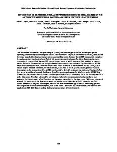
work. In the last section we will g ive our simulation and results. II. SOFTWARE EFFORT EST IMATION Software estimates are the basis for pro ject bidding, budgeting and planning. These are crit ical practices in the software industry, because poor budgeting and planning often has dramatic consequences. When budgets and plans are too pessimistic, business opportunities can be lost, while over-optimis m may be followed by significant losses [1]. Software effort estimation is the process of predicting the most realistic use of effort required to develop or maintain software. Effort estimates are used to calculate effort in work-months (WM) for the Soft ware Develop ment work elements of the Work Breakdown Structure (W BS). So ftware estimation can be modeled as the three stages, 1st stage involves size estimation, 2nd stage includes effort estimation, and time estimation, follo wed by the 3rd stage as cost estimation, and staffing estimation. Figure 1 shows the interaction between these modules in a typical software estimation process in Software Develop ment Life Cycle [10]. Effort Estimation Size Estimation
Ti me Estimation
Cost Estimation Staffing Estimation
Delphi Method: The technique is designed as a group communicat ion process which aims to achieve a convergence of opinion on a specific real-world issue. Here a group is made out of most experience people in the organizat ion. It overcomes the disadvantages of Expert Judg ment. 2. Algorith m Based Estimation- As the new technologies evolves and the software size became huge, the Judgment based estimation fails to predict correctly. So need of some formula based estimation techniques comes into picture. It is also of two types. COCOMO: The Constructive Cost Model (COCOM O) is an algorith mic estimation model developed by Barry W. Boeh m. The most fundamental calculation in COCOMO is the use of Effort equation to estimate the number of Person -Months required to develop a project.
Effort
A * ( size ) B
Where A is proportionality constant and B represents economy. Values of A and B depends upon the type of projects. A project can be classified into three types -Organic projects those involve small teams with good experience, Semi-detached projects those having mediu m teams with mixed experience working and embedded projects which are developed within a set of tight constraints. TABLE I VALUES OF ‘A’ AND ‘B’ IN COCOMO
Software Pro ject Fig. 1 Cycle
Sequence of estimates in Software Development Life
According to the last research reported by the Brazilian Ministry of Science and Technology-MCT, in 2001, only 29% of the companies accomp lished size estimation and 45.7% accomplished software effort estimate [2], so effort estimation has motivated considerable research in recent years. Effort Estimation Techniques Due course of time there are so many techniques evolved for effort estimat ion. Basically those can be categorized into three types1. Judgment Based Estimation 2. A lgorith m Based Estimat ion 3. Analogy Based Estimation 1. Judg ment Based Estimat ion- This is the most traditional and most popular estimation technique. In this all the estimations are made by human beings and dependent upon personal experience. It is of two types Expert Judgment: The mostly widely used cost estimation technique. It is an inherently top-down estimation technique. It relies on the experience, background, and business sense of one or many key people in the organization. This technique is risky because someone may overlook at some factors that make the new projects significantly different. Also the experts making estimate may not have the experience in similar projects.
A
B
Organic
2.4
1.05
Semi-detached
3.0
1.12
Embedded
3.6
1.20
Function Point Analysis (FPA): Function Point Analysis was developed by Alan Albercht of IBM in 1979. Function point metrics provide a standardized method for measuring the various functions of a software application. Depending upon this we can estimate our effort. Here all the functions are categorized in five types. Those are, Internal Logical File (ILF), External Interface File (EIF), External Input (EI), External Output (EO), and External Inquiry (EQ). For each category values assigned are low, mediu m or high. Besides the above mentioned domain values, fourteen co mplexity factors like Bach up and recovery, Data Co mmunication etc. are g iven certain values as per software requirement and final estimate is calculated. Function Points are simp le to understand, easy to count, require little effort and practice. [18] 3. Analogy Based Estimation- Analogy-based estimation has recently emerged as a pro mising approach, with comparable accuracy to algorith mic methods in some studies, and it is potentially easier to understand and apply. An estimate of the effort to complete a new software project is made by analogy with one or mo re previously co mpleted projects. Ease of use may be an important factor in the successful adoption of
estimation methods within industry, so analogy-based estimation deserves further scrutiny. There are many techniques those comes under analogy based estimat ionCase Base Reasoning: CBR is able to utilize the specific knowledge of previously experienced, concrete problem situations (cases). A new problem is solved by finding a similar past case, and reusing it in the new problem situation. A second important difference is that CBR also is an approach to incremental, sustained learning, since a new experience is retained each time a prob lem has been s olved, making it immed iately available for future problems. Artificial Neural Networks: Artificial Neu ral Networks (ANNs) is used in effort estimation due to its ability to learn fro m p revious data. It is also able to model co mplex relationships between the dependent (effort) and independent variables (cost drivers). In addition, it has the ability to generalize fro m the training data set thus enabling it to produce acceptable result for previously unseen data. III. A RT IFICIAL NEURAL NETWORKS Artificial Neural Network (ANN) is a massively parallel adaptive network of simple nonlinear co mputing element called Neurons, which are intended to abstract and model some of the functionality of the human nervous system in an attempt to partially capture some of its computational strengths [3, 13, and 14]. x1
bk
W k1
Activation function
x2
∑
W k2
..
..
xm
Output(Yk )
Uk
Aggregation Rule
W km
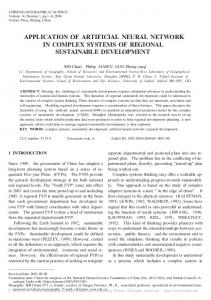
ANNs can be viewed as weighted directed graphs in which artificial neurons are nodes and directed edges (with weights) are connections between neuron outputs and neuron inputs. In mathemat ical notation, any neuron-k can be represented as follows: m
Wkj X j
j 1
Artificial Neural Networks Architecture: Depending upon the architecture the ANNs can be categorized into following types, as shown below [19]: (1)Feed-forward networks- A feed-forward ANN is the architecture in which the network has no loops. A feed-forward networks can again categorized into following(a) Single-layer perceptron- A single layer perceptron consists of a single layer of output nodes, the inputs neurons are connected directly to the outputs neurons via a series of weights. (b) Mu ltilayer perceptron- In mu lti-layer perceptron an additional layer of neurons present between input and output layers. That layer is called hidden layer. Any number of hidden layers can be added in an ANN depending upon the problem do main and accuracy expected. (c) Cascade network- Cascade network is a feed-forward neural network where the first layer will get signal fro m input. Each subsequent layer will receive signal fro m the input and all previous layers. (2) Elman Net works- It is a feed-fo rward network with partial recurrence. Elman NN is a special type of recurrent neural network where an additional set of “context units” is connected with the input layer. These are also connected with the hidden layer with connection weight one. The context unit works as memo ry for the network. (3)Recurrent/ Feed-back networks- In a recurrent (feed-back) ANN is an architecture in which loops occurs in the network.
Fig. 2 Architecture of an artificial neuron
Uk
error is calculated. In unsupervised train ing, the network is provided with inputs but not with desired outputs. The system itself must then decide what features it will use to group the input data [3].
and
Yk
(U k
bk )
where x1 ,x2 , …,xm are the input signals , wk1 ,wk2 ,….,wkm are the synaptic weights of the corresponding neuron, u k is the linear co mbiner output, b k is the bias, φ() is the activation function and y k is the output signal of the neuron. After an ANN is created it must go through the process of learning or t rain ing. The process of modifying the weights in the connections between network layers with the objective of achieving the expected output is called training a network. There are t wo approaches for training– supervised and unsupervised .In supervised training; both the inputs and the outputs are provided. The network then processes the inputs, compares its resulting outputs against the desired outputs and
Recurrent networks can have following types (a) Co mpetit ive networks- This neural networks is designed based on Competitive learning. Th is rule is based on the idea that only one neuron from a given iteration in a given layer will fire at a t ime. Weights are adjusted such that only one neuron in a layer, for instance the output layer, fire. Co mpetitive learning is useful for classification of input patterns into a discrete set of output classes . (b) Kohonen’s neural networks - The Kohonen’s neural networks differ considerably fro m feed-forward neural networks because it doesn’t have any activation function and also it doesn’t have a bias weight. It uses unsupervised learning for classification of input pattern presented to it. (c) Hopfield networks- It is a fully recurrent network. The network is based on Hebb’s Rule for learning. It can recall a memo ry, if presented with a corrupt or inco mplete version of data. (d) A RT models- This neuron networks works according to adaptive resonance theory (ART).The theory has led to neural models for pattern recognition and unsupervised learning.
These models are capable of learn ing stable recognition categories. ART networks are fu lly-connected networks, in that all possible connections are made between all nodes.
abstraction .It is a top-down approach. Design & analysis documents are UML diag rams. Metrics used are no. of classes, weighted method/class (WMC), UM L points...
IV. A NN IN EFFORT EST IMATION
3. Agile So ftware: Iterative and incremental development. Requirements and solutions evolve throughout the life cycle. Very popular now-a-days. All design documents are written in form of stories. Story points and sprints are used as metrics.
Artificial Neural Net work is used in effort estimat ion due to its ability to learn fro m previous data. It is also able to model complex relationships between the dependent (effort) and independent variables (cost drivers). In addition, it has the ability to generalize fro m the train ing data set thus enabling it to produce acceptable result for previously unseen data. Most of the work in the application of neural network to effort estimation made use of feed-forward multi-layer Perceptron, Back-propagation algorith m and sig moid function. However many researchers refuse to use them because of their shortcoming of being the “black bo xes” that is, determining why an ANN makes a particular decision is a difficult task. But then also many different models of neural nets have been proposed for solving many co mplex real life p roblems [4]. To use ANN for effort estimation we have to follow these stepsSteps in effort estimation 1. Data Collection: Collect data for prev iously developed projects like LOC, method used, and other characteristics. 2. Division of dataset: Divide the nu mber of data into two parts – training set & validation set. 3. ANN Design: Design the neural network with number of neurons in input layers same as the number of characteristics of the project. 4. Training: Feed the training set first to train the neural network. 5. Validation: After training is over then validate the ANN by giv ing the validation set data. 6. Testing: Finally test the created ANN by feeding test set data. 7. Error calculation: Check the performance of the ANN. If satisfactory then stop, else again go to step (3), make some changes to the network parameters and proceed. Once the ANN is ready we can g ive the parameter of any new project, and it will output the estimated effo rt for that project. V. TYPES OF SOFTWARE Software types can be categorized into: 1. Conventional/Procedure Oriented Software: Here the total project is d ivided into modules. All modules are developed separately. Then they are integrated to build complete software .Design & analysis documents are DFD and State-chart diagram. Metrics used are LOC, FPs, and COCOM O cost drivers. 2. Ob ject Oriented Soft ware: Pro ject is developed taking OBJECT as main entity. OO features availab le, inheritance,
4. Co mponent Based Software: In CBSD the total software is developed in forms o f components. “A co mponent is a coherent package of software that can be independently developed and delivered as a unit, and that offers interfaces by which it can be connected, unchanged, with other co mponents to compose a larger system.” Here the metrics used are component intensity, concurrency, frag mentation, etc. 5. Web Based Software: A web application is an application that is accessed over a network such as the Internet or an intranet. The term may also mean a computer software application that is coded in a browser-supported language (such as JavaScript, combined with a browser-rendered markup language like HTM L) and reliant on a common web browser to render the application executable.
Conventional
TABLE II KEY FEATURES OF DIFFERENT SOFTWARE Object Agile Component Web Based Oriented Software Based Software Software Software
-procedure
-method
-record
-object
-module
-class
-procedure call
-message
-LOC
-Use case points
-FPs
-CPs
-business value delivered
-Intensity
-story points
-Fragmentation
-sprint
-Project Experience
-Concurrency
-http count -page count
-Component
VI. RELAT ED WORKS We have reviewed works based on use of artificial neural networks in prediction of effort for Conventional Software and then for Object Oriented Software. First we present the conventional software develop ment effort estimation, followed by object oriented software. A. Conventional Software Review G. E. W ittig, et al. [5] used a dataset of 15 commercial systems, and used feed-forward back-propagation mu ltilayer neural network for his experiment. He had tried for numbers of hidden layers fro m 1-6, but found the best performance for only one hidden layer. Sig moid function was used. He found that for smaller system the error was 1% and for larger systems error was 14.2% of actual effort. In a paper by Ali Idri, et al. [4] he has used COCOM O-81 dataset and three layered back-propagation ANN, applying 13 cost drivers as inputs. Develop ment effort taken as output. By
taking 13 neurons in hidden layer and after 300,000 iterations he found, average MRE is 1.50%.
Simp le FPA and COCOM O model will not work for estimation of OO software.
F. Barcelos Tronto, et al. [2], also used COCOM O-81 dataset, but he has taken only one input, i.e TOTKDSI (thousands of delivered source instructions). All the input data were normalized to [0, 1] range. Here a feed-forward mu ltilayer back-propagation ANN was used with the 1-9-4-1 architecture. The performance in MM RE found was 420, where as that of COCOMO and FPA was 610 and 103 respectively.
Gennaro Costagliola, et al. [15] had proposed the concept of Class Point. In this approach he had presented a FPA like approach for OO software project. He had used two measurements of size, CP1 & CP2. CP1 is for estimation at the beginning stage of development and CP2 is for later refinement when more informat ion is available. He had considered three metrics No. of External Methods (NEM), No. of Service Routines (NSR) and No. of Attributes (NOA) to find the complexity of a class. Here he had proposed 18 system characteristics to find Technical Co mplexity. Fro m the experiment over 40 pro ject dataset he found that the aggregated MMRE of CP1 is 0.19 and CP2 is 0.18.
Jaswinder Kaur, et al. [6] implemented a back-propagation ANN of 2-2-1 architecture on NASA dataset consist of 18 projects. Input was KDLOC and development methodology and effort was the output. He got result MMRE as 11.78. Roheet Bhatnagar, et al. [7] used MATLAB NN toolbox for effort predict ion. He had used a dataset proposed by Lopez-Martin, which consists of 41 projects data. He has designed a 3-3-1 neural network, applied the Dhama Coupling (DC), McCabe Co mplexity (M C) and Lines of Code (LOC) as inputs. Development time was the only one output. Fro m the experiment he found that the percentage of error during training, validation and testing was between +14.05 to -25.60, +12.76 to -18.89 and +13.66 to -15.75 respectively. K.K. Aggarwal, et al. [8] had investigated for finding the best training algorithm. Here ISBSG repository data was used on a 4-15-1 feed-forward ANN. Four inputs were taken-FP, FP standard, language and maximu m team size. SLOC was the only output. He had tried all t rain ing algorithm and concluded that ‘trainbr’ is the best algorithm. ‘traingd’ was found to be the next best algorith m.
VII. PERFORMANCE CRIT ERIA
TABLE III RELATED WORKS Author
Learning Algorithm
Dataset
No. of Projec ts
No. of Inputs
ANN Configuration
G. E. Wittig[5]
Back-prop agation
Commercial Systems
15
-
[23-4-1]
Ali Idri [4]
Back-prop agation
COCOMO
63
13
[13-13-1]
I.F. Barcelos Tronto [2]
Back-prop agation
COCOMO
63
1
[1-9-4-1]
Jaswinder Kaur[6]
Back-prop agation
NASA
18
2
[2-2-1]
Rpheet Bhatnagar[7]
Back-prop agation
Lopez-Martin
41
3
[3-3-1]
K.K. Aggarwal [8]
Back-prop agation
ISBSG
88
Then Wei Zhou and Qiang Liu [16] in the year 2010 have extended the above paper in two ways. First they have added a size measurement named CP3 based on CPA. Second, in-order to improve the precision of estimation, they have taken 24 system characteristics instead of 18 in the previous one. Fro m this they found that where the original CP1 gives MMRE 0.22, this give 0.19 and incase of CP2 it was 0.18, now it is 0.14. S.Kan mani, et al. [17] has used the same CPA with a little change, by using neural network in mapping the CP1 and CP2 into effort. In the base paper of Gennaro [15], he had used regression method to find the values of the constants that can be mu ltiplied and added with computed CP1 and CP2 to find the effort. Here in this paper Kan mani has used neural network to find those values. The aggregate MMRE is imp roved fro m 0.19 to 0.1849 for CP1 and fro m 0.18 to 0.1673 for CP2.
4
There are many performance criteria to evaluate the accuracy of any estimat ion. The Mean Magnitude Relative Error (MM RE) is a widely-accepted criterion in the literatures which is based on MRE. Root Mean Square Erro r (RMSE) is the next most popular evaluation criteria. In some of the papers Pred ( ) and BRE are also used for measuring the accuracy. A. Mean Magnitude Relative Error (MMRE) MMRE is frequently used to evaluate the performance of any estimation technique. It measures the percentage of the absolute values of the relative errors, averaged over the N items in the "Test" set and can be written as [6]:
MMRE
1 N
N i 1
( yi
yˆ i ) yi
[4-15-1]
B. Object- Oriented Software Review Object oriented technology is becoming very popular now-a-days, because of the features offered by it like Encapsulation, Inheritance, Poly morphis m, etc. Modern software development technologies such as .Net and Java are rich of features hose are capable of developing highly maintainable, reusable, testable and reliable software [19].
where represents the ith value of the actual effort and is the estimated effort. The M RE calcu lates each project in a dataset while the MMRE aggregates the mult iple projects . The model with the lowest MMRE is considered the best. B. Root Mean Square Error (RMSE) RMSSE is another frequently used performance criteria which measures the difference between values predicted by a model or estimator and the values actually observed from the thing being modeled or estimated. It is just the square root of the mean square error, as shown in equation given below [6]:
TABLE IV NASA DATA SET
RMSE
1 N
N i 1
( yi
yˆ i ) 2
C. Balance Relative Error (BRE) BRE is another evaluation criterion for accuracy [9]:
BRE(%) 100 * yi
yˆ i min( yi , yˆ i )
D. Pred(l) Another measure of Pred(l) was also adopted to evaluate the performance of the established software effort estimation models. It provides an indication of overall fit for a set of data points, based on the MRE values for each data point [19]:
Pr ed (l )
k N
where N is the total number of observations and k is the number of observations with MRE less than or equal to l. VIII. EXPERIMENTAL SETUP FOR EST IMATION
MC
DC
LOC
DT
1
0.25
4
13
1
0.25
10
13
1
0.333
4
9
2
0.083
10
15
2
0.111
23
15
2
0.125
9
15
2
0.125
9
16
2
0.125
14
16
2
0.167
7
16
2
0.167
8
18
2
0.167
10
15
2
0.167
10
15
2
0.167
10
18
2
0.2
10
13
2
0.2
10
14
Data Preparation
2
0.2
10
15
For simulation of conventional software projects we have used a standard dataset proposed by Lopez-Mart in et.al. [7]. It consists of 41 system develop ment projects data, where the Develop ment Time (DT), Dharma Coupling (DC), McCabe Co mplexity (M C) and the Lines of Code (LOC) metrices were registered, as shown in table-IV. Since all the programs we re written in Pascal, the module categories mostly belong to procedures and functions. The development time of each of the forty-one modules were reg istered including five phases: requirements understanding, algorithm design, coding, compiling and testing
2
0.2
15
13
2
0.25
10
12
2
0.25
10
12
3
0.083
17
22
3
0.125
11
19
3
0.125
15
18
3
0.125
15
19
3
0.143
13
21
3
0.143
14
20
3
0.143
14
21
3
0.143
15
19
3
0.143
15
20
3
0.167
13
15
3
0.167
14
13
3
0.2
18
19
3
0.25
9
13
3
0.25
12
12
3
0.25
17
12
4
0.077
16
21
4
0.077
31
21
4
0.111
16
19
4
0.2
24
18
5
0.143
22
24
5
0.143
22
25
5
0.2
22
18
In the next step we have experimented for effort estimation of object-oriented software. Here we have used data from 40 Java systems developed during two successive semesters . Detail data set is given in table-V.
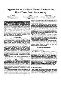
ANN Preparation In this experiment we have created one feed-forward neural network using MATLA B10 NN toolkit [12]. For the neural networks [3-5-1] architecture is used, i.e. 3 neurons in input layer, 5 neurons in hidden layer and 1 neuron in output layer, in table-VI. Train ing algorith m used is ‘trainlm’. For train ing the dataset is divided into three divisions -for training 80%, for validation 10% and fo r testing 10%. Learn ing rate is set at 0.01.Stopping criteria were set by number of epochs as 1000 and goal as 0.00. The ANN shown in fig.3 is created by MATLAB tool, will be applied to convention software dataset first and then the same one will be applied on object oriented software dataset.
TABLE V DATA SETS
TABLE VI ANN SUMMARY
Project No.
Effort
CP1
CP2
NEM
NOA
NSR
1
286
103.18
110.55
142
170
97
Layers
3
2
396
278.72
242.54
409
292
295
Input Neurons
3
3
471
473.9
446.6
821
929
567
Hidden Layer Neurons
5
4
1016
851.44
760.96
975
755
723
5
1261
1263.12
1242.6
997
1145
764
Output Neurons
1
6
261
196.68
180.84
225
400
181
Training
7
993
718.8
645.6
589
402
944
Training Function
Tansig
8
552
213.3
208.56
262
260
167
Algorithm
Back Propagation
9
998
1095
905
697
385
929
10
180
116.62
95.06
71
77
218
Training Function
TrainLM
11
482
267.8
251.55
368
559
504
Parameters
12
1083
687.57
766.29
789
682
362
Learing Rate
0.01
13
205
59.64
64.61
79
98
41
Epochs
1000
14
851
697.48
620.1
542
508
392
15
840
864.27
743.49
701
770
635
Error
0.00
16
1414
1386.32
1345.4
885
1087
701
17
279
132.54
74.26
97
65
387
18
621
550.55
418.66
382
293
654
19
601
539.35
474.95
387
484
845
20
680
489.06
438.9
347
304
870
21
366
287.97
262.74
343
299
264
22
947
663.6
627.6
944
637
421
23
485
397.1
358.6
409
451
269
24
812
676.28
590.42
531
520
401
25
685
386.31
428.18
387
812
279
26
638
268.45
280.84
373
788
278
27
18.3
2090.7
1719.25
724
1633
1167
28
369
114.4
104.5
192
177
126
29
439
162.87
156.64
169
181
128
30
491
258.72
246.96
323
285
195
31
484
289.68
241.4
363
444
398
32
481
480.25
413.1
431
389
362
33
861
778.75
738.7
692
858
653
34
417
263.72
234.08
345
389
245
35
268
217.36
198.36
218
448
187
36
470
295.26
263.07
250
332
512
37
436
117.48
126.38
135
193
121
38
428
146.97
148.35
227
212
147
39
436
169.74
200.1
213
318
40
356
112.53
110.67
154
147
Architecture
Fig. 3 The Feed-Forward ANN using M ATLAB
IX. EXPERIMENTAL RESULT S Conventional Software The feed-forward NN was trained for 10 iterations and then the development time was predicted. We have considered ten randomly chosen projects for performance comparison. TABLE VII COMPARISON OF MULTIPLE REG . AND ANN
Project No.
Actual DT
M ultiple Regression
M RE
Neural Network
M RE
3 4
9 15
8.2 18.2
0.09 0.21
9.31 16.01
0.03 0.07
183
5 14 19 20 21 34 35 39
15 13 12 22 19 12 21 24
16.62 14.34 12.7 19.91 18.83 14.41 22.22 21.81
0.11 0.10 0.06 0.10 0.01 0.20 0.06 0.09
14.85 14.57 12.53 21.06 20.64 12.9 20.58 24.2
0.01 0.12 0.04 0.04 0.09 0.08 0.02 0.01
83
MMRE
0.10
0.05
7
Table-VII presents comparison of prediction using mult iple regression and neural network and fig.4 shows the MRE performance of both the techniques.
TABLE IX AGGREGATED MMRE OF CP1, CP2 & ANN
Aggregate MMRE CP1
0.192
CP2
0.165
ANN
0.097
X. CONCLUSION
Fig. 4 M RE of M ultiple Regression & ANN
Object-Oriented Software After feeding data of 40 projects into the ANN and co mplet ing the training, then the ANN is used for prediction of results. We have partitioned the data into 4 sets taking 10 pro ject data in each one. Then these data sets were given to the ANN for calculating the efforts. The table-VIII & table-IX given below compares the prediction of our ANN with those of CP1 and CP2.
Estimation is one of the crucial tasks in software project management. There are different estimation techniques are present, but those are suitable for any one type of software development. We want to verify the applicability of A NN based estimation for software develop ment effort, in all types of software. In this paper we have tested with conventional and object oriented software. We have observed that it gives good results on both types of software in co mparison to mult iple regression and class points analysis. In further extension of this paper, we will test estimation with ANN design tool for effort estimation of Agile and Web-based software.
TABLE VIII COMP ARISON OF CP1, CP2 & ANN
Actual Effort
CP1
M RE
CP2
M RE
ANN
M RE
1
286
328.83
0.15
340.57
0.19
321.5
0.12
2
396
476.81
0.20
460.95
0.16
446.2
0.13
3
471
641.35
0.36
647.05
0.37
485.4
0.03
4 5
1016 1261
959.62 1306.66
0.06 0.04
933.75 1373
0.08 0.09
1012.8 1268.8
0.00 0.01
6
261
407.65
0.56
404.68
0.55
396.7
0.52
7 8
993 552
847.46 421.66
0.15 0.24
828.54 429.96
0.17 0.22
986.3 480.4
0.01 0.13
9
998
1164.94
0.17
1065.11
0.07
1016.5
0.02
10
180
340.16
0.89
326.45
0.81
163
0.09
MMRE
0.28
0.27
REFERENCES [1]
[2]
[3] [4]
0.11 [5]
[6]
[7]
[8]
F IG . 5 MM RE OF CP1, CP2 & ANN
Stein Grimstad, Magne Jorgensen, Kjetil Molokken-Ostvold ,”Software effort estimat ion terminology: The tower of Babel”, Elsevier, 2005. I.F. Barcelos Tronto, J.D. Simoes da Silva, N. Sant. Anna , “Co mparison of Artificial Neural Network and Regression Models in Software Effort Estimation”, INPE ePrint, Vo l.1, 2006. Simon Haykin, “Neural Net works: A Co mprehensive Foundation”, Second Edition, Prentice Hall, 1998. Ali Idri and Taghi M. Khoshgoftaar& Alain Abran,”Can Neural Net works be easily Interpreted in So ftware Cost Estimation”, IEEE Transaction, 2002, page:1162-1167. G.E. Wittig and G.R Finnic, “Using Artificial Neu ral Networks and Function Points to estimate 4GL software development effort”, AJIS,1994, page:87-94. Jaswinder Kaur, Satwinder Singh, Dr. Karanjeet Singh Kahlon, PourushBassi,“Neural Network-A Novel Technique for Software Effort Estimation”, International Journal of Co mputer Theory and Engineering, Vo l. 2, No. 1 February, 2010, page:17-19. Roheet Bhatnagar, Vandana Bhattacharjee and Mrinal Kanti Ghose, “Software Development Effort Estimat ion –Neural Network Vs. Regression Modeling Approach”, International Journal o f Engineering Science and Technology,Vol. 2(7), 2010,page: 2950-2956. K.K. Aggarwal, Yogesh Singh, Pravin Chandra and Manimala Puri, “Evaluation of various training algorith ms in a neural network model for software engineering applications” , ACM SIGSOFT So ftware Eng ineering , July 2005, Vo lu me 30 Nu mber 4 , page: 1-4. 8
[9]
[10]
[11] [12]
[13]
[14] [15]
[16]
[17]
[18]
[19]
Mrinal Kanti Ghose, Roheet Bhatnagar and Vandana Bhattacharjee , “Co mparing So me Neural Net work Models for Software Develop ment Effort Predict ion” , IEEE, 2011. Jagannath Singh and Bibhudatta Sahoo, ”Software Effort Estimation with Different Artificial Neu ral Network”, IJCA Special Issue on 2nd National Conference- Co mputing, Co mmunicat ion and Sensor Network (CCSN) (4):13-17, 2011. Satish Kumar, “Neural Networks: A Classroom Approach”, Tata McGraw-Hill, 2004. Howard Demuth and Mark Beale, “Neural Network Toolbox-For use with MATLAB”,User’s Gu ide,Version-4,Page-5.28. N.K.Bose and P.Liang, “Neural Network Fundamentals with Graphs, Algorithms and Applications”, Tata McGraw Hill Ed ition,1998. B. Yegnanarayana, “Artificial Neural Net works”, Prentice Hall of India, 2003. Gennaro Costagliola and Genoveffa Tortora, “Class Point: An Approach for the Size Estimat ion of Object-Oriented Systems”, IEEE TRANSACTIONS ON SOFTWARE ENGINEERING, VOL. 31, NO. 1, JA NUA RY 2005,page 52-74 Wei Zhou and Qiang Liu,” Extended Class Point Approach of Size Estimation for OO Product”, IEEE sponsred 2nd International Conference on Co mputer Engineering and Technology,2010,Vo l-4 ,Page:117-122. S. Kan mani, J. Kathiravan, S. Senthil Ku mar and M. Shanmugam,” Neural Net work Based Effort Estimat ion using Class Points for OO Systems”,IEEE-International Conference on Co mputing: Theory and Application(ICCTA’07),2007. Magne Jørgensen and Torleif Halkjelsvik, “The Effects of Request Formats on Judgment-based Effort Estimat ion”, Journal of Systems and Software, vol. 83, 2010, pp. 29-36. Mehwish Nasir, “ A Survey of Soft ware Estimat ion Techniques and Project Planning Pract ices”, Seventh ACIS International Conference on So ftware Engineering,Artificial Intelligence, Net working, and Parallel/Distributed Co mputing (SNPD’06), IEEE,2006.
Jagannath Singh is a M.Tech research scholar at National Institute of Technology Rourkela India. He had received B.E from Biji Pattnaik University of Technology, Orissa. His research interest includes Software Engineering, Artificial Neural Networks and Microprocessor.
Bibhudatta Sahoo received the M.Sc. Engineering in Computer Science from National Institute of Technology Rourkela, INDIA, in 1999. He is currently an assistant professor in the Department of Computer Sc. & Engineering, NIT Rourkela, India. His interest include Parallel & Distributed Systems, Networking, Computational Machines, System Sof tware, High performance Computing, VLSI algorithms He is a member of the IEEE Computer Society & ACM.
9