Strojarstvo 51 (4) 313-321 (2009)
K. ŠIMUNOVIĆ et. al., ������������������������������������������������ Application of Artificial Neural Networks...���� 313
CODEN STJSAO ZX470/1390
ISSN 0562-1887 UDK 658.78.012.12:519.8:004.032.26
Application of Artificial Neural Networks to Multiple Criteria Inventory Classification Katica ŠIMUNOVIĆ, Goran ŠIMUNOVIĆ and Tomislav ŠARIĆ Strojarski fakultet u Slavonskom Brodu Sveučilišta J. J. Strossmayera u Osijeku (Mechanical Engineering Faculty, J. J. Strossmayer University of Osijek), Trg Ivane Brlić-Mažuranić 2, HR35000 Slavonski Brod, Republic of Croatia
[email protected] Keywords Analytical hierarchy process Artificial intelligence Multiple criteria inventory classification Neural network Ključne riječi Analitički hijerarhijski proces Neuronske mreže Umjetna inteligencija Višekriterijska klasifikacija zaliha Received (primljeno): 2008-15-11 Accepted (prihvaćeno): 2009-05-31
Original scientific paper Inventory classification is a very important part of inventory control which represents the technique of operational research discipline. A systematic approach to the inventory control and classification may have a significant influence on company competitiveness. The paper describes the results obtained by investigating the application of neural networks in multiple criteria inventory classification. Various structures of a back-propagation neural network have been analysed and the optimal one with the minimum Root Mean Square error selected. The predicted results are compared to those obtained by the multiple criteria classification using the analytical hierarchy process.
Primjena umjetnih neuronskih mreža u višekriterijskoj klasifikaciji zaliha Izvornoznanstveni članak Klasifikacija zaliha predstavlja značajan dio upravljanja zalihama kao jedne od tehnika operacijskih istraživanja. Sustavni pristup upravljanju i klasifikaciji zaliha može imati značajan utjecaj na tržišnu konkurentnost tvrtke. U radu su opisani rezultati istraživanja primjene neuronskih mreža za višekriterijsku klasifikaciju zaliha. Analizirane su različite strukture neuronske mreže širenja unazad, te izabrana optimalna struktura s najmanjom razinom srednjeg kvadratnog odstupanja. Rezultati dobiveni neuronskim mrežama uspoređeni su s rezultatima višekriterijske klasifikacije zaliha dobivenim primjenom metodologije “analitički hijerarhijski proces”.
1. Introduction Inventory or stock control is a part of operational research discipline. Inventory control helps to make a decision about the appropriate quantity of inventory at the appropriate time. The main questions are: how much and when. Classification of inventory is very important too. Because of the huge number of inventory items in many companies, great attention is directed to inventory classification into the different classes, which consequently require the application of different management tools and policies. ABC analysis is a very popular and the most widely used analytical method for inventory classification. By the ABC analysis, items are classified into three classes: A, B and C. Class A represents the class of the most important items, while class C is the class with the lowest importance, according to the predefined criterion. Very often, this criterion is the annual cost usage, obtained by the multiplication of
annual demand and average unit price. There are some other criteria like average unit price, the number of orders, purchasing conditions and some other. Sometimes, only one criterion is not a very efficient measure for decision-making. Therefore, multiple criteria decision making methods are used. Consequently, the term multiple criteria inventory classification is used. Other criteria, except for the annual cost usage, are as follows: lead time of supply, part criticality, availability, average unit price, stock out penalty costs, etc. So many different methods for classifying inventory and taking into consideration multiple criteria have been used and developed. Among them, artificial intelligence methods like neural networks, fuzzy logic and genetic algorithms are applied. An artificial intelligence concept is based on the development of the intelligent computer systems with properties similar to human intelligence. Neural networks have been widely applied to problem
314
K. ŠIMUNOVIĆ et. al., Application of Artificial Neural Networks...
Symbols/Oznake
Vri
Strojarstvo 51 (4) 313-321 (2009)
- the overall score for the i-th alternative (i = 1, …, m) - ukupni iznos za i-tu alternativu (i = 1, …, m)
Bj
- weighting factor for the j-th criterion (j = 1, …, n) - težinski faktor za j-ti kriterij (j = 1, …, n)
dn
- desired value of a neural network n-th output - željena vrijednost n-tog izlaza neuronske mreže
Xi
- input variables - ulazne varijable
E
- global error - ukupna grješka
xij
- value of the j-th criterion of the i-th alternative - vrijednost j-tog kriterija za i-tu alternativu
- the error that propagates backwards through all the layers - grješka koja se širi unazad kroz sve slojeve mreže
xij*
- transformed value of the j-th criterion of the i-th alternative - transformirana vrijednost j-tog kriterija za i-tu alternativu
G
- the function increment - prirast funkcije
max xij
- maximum value of the j-th criterion among i alternatives - maksimalna vrijednost j-tog kriterija među i alternativa
Y0
- output variables - izlazne varijable
ycj
- the output value of neuron j - vrijednost izlaza neurona j
min xij - minimum value of the j-th criterion among i alternatives - minimalna vrijednost j-tog kriterija među i alternativa
ydi
- the actual (desired) output - stvarni (željeni) izlaz
yn
- neural network n-th output - n-ti izlaz neuronske mreže
α
- learning coefficient - koeficijent učenja
MS
- mean square error - srednje kvadratno odstupanje
N
- number of pairs of the training set input-output values - broj parova ulazno-izlaznih vrijednosti skupa za učenje
RMS
- root mean square error - korijen srednjeg kvadratnog odstupanja
SVij
- scaled j-th criterion value for the i-th alternative - skalirana vrijednost j-tog kriterija za i-tu alternativu
T
- the function threshold - prag funkcije
solution in production factories: in the procedures of the determination of optimal cutting conditions [1-2], tool path generation [3], surface roughness prediction [4], tool wear monitoring [5], prediction of technological time [6], maintenance planning [7], etc. The authors [8], use neural networks to classify inventory. Unit price, ordering cost, demand range and lead time represent input neurons. A, B and C classes represent the output layer. As learning tools genetic algorithm and back propagation algorithm are used and compared. In the paper [9], principal component analysis is compared with a hybrid model combining principal component analysis with artificial neural network and back propagation algorithm. Chu et al. [10], have suggested a new inventory classification approach called ABC-fuzzy classification combining the traditional ABC with fuzzy
Δ
- weights - težine
- output state of the j-th neuron in the s-th layer - izlazno stanje j-tog neurona u s-tom sloju
- increase in the network weighted connections - prirast težina veza u mreži
Δwji
- the value of the difference in the weights of neuron j and neuron i - vrijednost razlike težina neurona j prema neuronu i
εi
- error - grješka
classification. The authors [11], applied genetic algorithm technique to the problem of multiple criteria inventory classification. Their proposed method is called Genetic Algorithm for Multicriteria Inventory Classification and it uses genetic algorithm to learn the weights of criteria. After the weights are obtained by genetic algorithm, the total score for each item is calculated, similar to analytic hierarchy process methodology (AHP further). AHP methodology was developed by Thomas Saaty [12-13]. This methodology is based on the decomposition of the defined decision problem to the hierarchy structure which consists of the main goal at the top of the hierarchy followed by the criteria and sub-criteria (also sub-subcriteria) and finally by the alternatives at the bottom of the hierarchy. In the papers [8, 14], an AHP methodology has been used to classify inventory. Both quantitative
Strojarstvo 51 (4) 313-321 (2009)
K. ŠIMUNOVIĆ et. al., ������������������������������������������������ Application of Artificial Neural Networks...���� 315
and qualitative criteria can be taken into consideration. Calculated criteria weights and alternative priorities (preferences) are used to rank the alternatives (inventory items or stock keeping units). The authors [15] suggested a model based on the ranking by the distances from the positive and negative ideal solution. It seems to be a TOPSIS method which together with the AHP methodology belongs to multiple attribute decision making methods. The first step of this method is to present the whole population (all of the items) by the three representative case sets for classes A, B and C. Further, quadratic distances of the case sets criteria data from the minimal and maximal value of the whole population should be calculated. These values are the basis for formulation of a quadratic nonlinear model with the quadratic objective function to be minimised, subjected to the constraints of distances RA, RB and RC. Items with a distance smaller than RA, are sorted to class A. Items with a distance greater than RA, and smaller than RB, are classified to class B. Finally, items with a distance greater than RB, are classified into class C. Bhattacharya et al. [16], have also used a TOPSIS method to classify inventories into classes. Flores et al. [17-18] has transformed the traditional ABC analysis for the inventory classification, taking into consideration another relevant i.e. significant criterion. This method, the so called bi-criteria inventory classification, uses the traditional ABC analysis to classify inventory by the first criterion, and then by the second criterion. The main disadvantage of this method is that the weights of the two criteria are assumed to be equal. A weighted linear optimization model is developed, which is based on the concept of data envelopment analysis (DEA) [19]. The weighted additive function (score) is used, which includes all the performances in terms of different criteria for an item. An optimization linear model is defined for each item. By solving this model, the optimal inventory score for each item, as well as weighted factor values (weights) for all the criteria are generated. For a large number of items, this method is time consuming, but it provides an objective way of determining the weights. The author [20] proposes a very similar, but simplified model to Ramanathan,s model. This approach does not require a liner optimizer to solve the model. All the criteria data for each alternative are transformed and normalised to the scale from 0 to 1. The partial averages of the transformed criteria values are calculated then for all items. The next step is to choose the maximal partial average value for each item and rank the items by these values. The traditional ABC analysis is then applied. The authors [21] presented an extended version of the Ramanathan,s model with the main aim of avoiding the classification of the items with the high value of an unimportant criterion, to class A.
Further, the paper is organised as follows. In section 2, AHP methodology is described in general and the AHP model with four criteria for ranking 432 inventory items is given. Part 3 of the paper deals with the application of artificial neural network to inventory classification which uses four input variables (four criteria) and three output variables (the classes A, B and C). The results obtained by these two methods are compared and suggestions for further investigations are given in the last part of the paper.
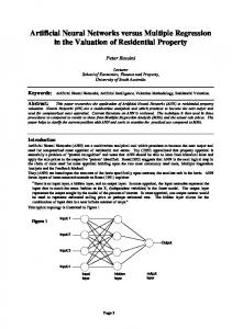
2. Inventory classification by the AHP methodology 2.1. AHP methodology – general model AHP methodology is based on decomposition of the defined decision problem to the hierarchy structure. The hierarchy structure is a tree-like structure which consists of the main goal at the top of the hierarchy (the first level), followed by the criteria and sub-criteria (also subsub-criteria) and finally by the alternatives at the bottom of the hierarchy (the last level), Figure 1.
Figure 1. AHP model with “n” criteria and “m” alternatives Slika 1. AHP model s “n” kriterija i “m” alternativa
The goal represents the optimum solution to the decision problem. It can be the selection of the best alternative among many feasible alternatives. Also, the ranking of all alternatives can be performed, by obtaining the priorities. Criteria (sometimes called objectives or attributes) are the quantitative or qualitative data (judgements) for evaluating the alternatives. The weights of the criteria represent the relative importance of each criterion compared to the goal. Finally, alternatives represent the group of feasible solutions of the decision problem. Alternatives are evaluated against the set of criteria. AHP methodology has three basic steps: • Decomposition of the defined decision problem to the hierarchic structure - building an AHP model
316
•
•
Strojarstvo 51 (4) 313-321 (2009)
K. ŠIMUNOVIĆ et. al., Application of Artificial Neural Networks...
with the overall goal, the evaluation criteria (subcriteria) and alternatives. Pair wise comparisons of the criteria and alternatives based on the Saatys scale of numbers from 1 to 9, Table 1. The value 1 means equal importance of two criteria (alternatives), while the value 9 stands for extreme importance of one criterion (alternative) to another. Pair wise comparisons of the criteria are performed with respect to the goal or criteria at a higher level. The weights of the criteria represent the ratio of how much more important one criterion is than another, with respect to the goal or criterion at a higher level. Pair wise comparisons of the alternatives are performed against each criterion and represent the ratio of how much more important one alternative is than another, taking into account each criterion. The local priorities of alternatives are derived. Testing the consistency of subjective judgements is also performed. Synthesising the results by calculation of the total priorities of alternatives. The total priority of each alternative is calculated by the multiplication of the local priority of alternative by the weight of corresponding criterion and then summing all the products for each criterion. Sensitivity analysis can also be performed and it gives the response of the alternative priorities to the change of the input data.
Table 1. Saaty’s scale for pair wise comparisons Tablica 1. Saatyeva ljestvica za usporedbu u parovima Scale / Ljestvica 1 3 5 7 9 2, 4, 6, 8
Description of the importance / Opis intenziteta važnosti equal / jednako važno moderate / umjereno važnije strong / važnije very strong / puno važnije extreme / ekstremno važnije intermediate values / međuvrijednosti
In AHP methodology, for a very large number of alternatives, making pair wise comparisons of alternatives, with respect to each criterion, can be time consuming and confusing, because the total number of comparisons will also be very big. Therefore, instead of pair wise comparisons of alternatives, relative priorities can be obtained by scaling (normalizing, transforming) the alternative data for each criterion. The data (qualitative or quantitative) can be transformed in different ways. Transformations of criteria data on the alternatives can be performed according to different formulas. The vector normalization is one of the transformation techniques where each j-th criteria data is divided with its norm. In linear transformation each positively related j-th criteria data is divided by the maximum data of the j-th
column of decision matrix. In linear transformation, for negatively related criteria, each j-th criteria data is put into the relation with the minimum data of the j-th column of a decision matrix. For the positively related criteria, the greater value of criteria means more importance. On the other hand, for the negatively related criteria, the smaller value of criteria means more importance. There is also the modification of linear transformation which gives, for positive criteria, the following expression: ,
(1)
while, for the negative criteria, the following expression is given: .
(2)
All the criteria data are transformed to the 0 - 1 scale. Scaled value of the j-th criterion (SVij) for the i-th alternative is multiplied by the weighting factor (or simply weight) of the j-th criterion (Bj). The sum of multiplied scaled values and weighting factors across all of the criteria (so called weighted sum) represents the overall score for the alternative item (see the expression 3). The alternative with the maximum score is on the top, while the alternative with the minimum score is on the bottom of the ranking scale. (3) 2.2. Application of the AHP methodology to inventory classification This part of the paper illustrates the application of AHP methodology for ranking and classifying items into classes A, B and C. 432 items for the assembly of the part of agricultural machine have been quantitatively analyzed. For multiple criteria inventory classification, four criteria were included. All the criteria are positively related to the importance level. The criteria are as follows: • Annual cost usage, €/year (calculated by multiplying the annual demand and the average unit price), • Criticality factor (rated from 1 – noncritical to 5 – extremely critical), • Lead time 1, working days – this is an interval from the ordering till the receiving of items for the development of a new product and start up of batch production.
Strojarstvo 51 (4) 313-321 (2009)
•
K. ŠIMUNOVIĆ et. al., ������������������������������������������������ Application of Artificial Neural Networks...���� 317
Lead time 2, working days – this is an interval from the ordering till the receiving of items for the batch production when the new product is already developed. The lead time 2 is equal to or shorter than lead time 1, because the development phase is missing.
Multiple criteria inventory classification is carried out by using the modified AHP methodology, which includes pair wise comparisons of criteria, but not pair wise comparisons of alternatives. The AHP model is shown in Figure 2. Criteria weights are derived from the pair wise comparisons according to the Saaty scale (Table 2). The following considerations about the criteria given by the experts in this field are significant. The criterion criticality is very important because of the serious consequences of not having a part when it is needed for the assembly. Lead time 2 is more important than lead time 1, because of planning and scheduling the batch production. From the technical and manufacturing point of view, annual cost usage criterion is less important, but for the purchasing unit it is more important.
Calculated weights of criteria are as follows: B1=0,224 (the weight of the first criterion-annual cost usage), B2=0,431 (the weight of the second criterion-criticality), B3=0,138 (the weight of the third criterion-lead time 1) and B4=0,207 (the weight of the fourth criterion-lead time 2). Because of the large number of alternatives (432), pair wise comparisons of the alternatives are not performed (as in original AHP methodology). Instead of that, transformation of the criteria data of alternatives is made by using the expression (1). Overall score for each alternative (item) across all four criteria is calculated using the expression (3). Items are ranked according to overall scores in the descending order. The limits for the classes are derived on the following basis. Class A involves 20 % of the total amount of items. Class B involves another 20 % of the total amount of items, while 60 % of items belong class C.
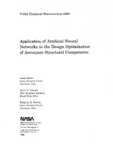
3. Inventory classification by backpropagation neural network 3.1. Selection of type of neural network – general model The observed research belongs to the problems dealing with continuous input and output values i.e. problems connected with prediction; thus the back-propagation network is applied. Figure 3 shows the structure of a back-propagation network with one hidden layer (there can be more hidden layers), while the structure of an artificial neuron is shown in Figure 4.
Figure 2. AHP model Slika 2. AHP model
Table 2. Pair wise comparisons of criteria Tablica 2. Uspoređivanje kriterija u parovima Criticality / Kritičnost
Lead time 1 / Vrijeme isporuke 1
Lead time 2 / Vrijeme isporuke 2
Annual cost usage / Godišnji trošak
1/2
2
1
Slika 3. Struktura mreže širenja unazad
Criticality / Kritičnost
-
2
3
During the process of learning the aim is to enable fast convergence and reduce global error given by (4):
Lead time 1 / Vrijeme isporuke 1
-
-
1/2
Figure 3. Structure of a back-propagation network
.
(4)
In this type of network global error propagates backwards through the network all the way to the input
318
K. ŠIMUNOVIĆ et. al., Application of Artificial Neural Networks...
layer. During the backward pass all weighted connections are adjusted in accordance with the desired neural network output values. An increase or decrease of actual values of the weights
affects the decrease of global error.
Strojarstvo 51 (4) 313-321 (2009)
The weights in the network can be updated for each learning vector separately or else cumulatively, which considerably speeds up the rate of learning (convergence). Therefore the objective of the learning process in a neural network is to achieve the lowest possible level of error between the outputs obtained by training the network and the actual (desired) results. This is realized by adjusting the weights of the neurons, and by accepting the objective function, defined below through minimization of the mean square error. A general form vector of the model applicable for a neural network input is as follows: ,
where vector Xi = {xi1, xi2, xi3,..., xin} represents input variables, and vector Yo = {yo1, yo2, yo3,..., yon}output variables.
Figure 4. Model of a neuron structure [22] Slika 4. Model strukture neurona [22]
Through application of the gradient descent rules the increase in the network weighted connections be given as: ,
can (5)
where α is the learning coefficient. Derivations given above can be calculated as: .
3.2. Application of back-propagation network to inventory classification In the given problem the model vector has three output variables – classes A, B and C. Input variables are: annual cost usage, criticality factor, lead time 1 and lead time 2, previously described in part 2.2 of the paper. Variables with a value range for the proposed model are given in table 3. Table 3. Variables with a value range for the proposed model
(6)
The value of the weighted connections increase in the network Δ
(10)
Tablica 3. Varijable s vrijednostima protezanja za predloženi model No. / Br.
is now: ,
(7)
where α is the learning coefficient, represents output state of the j -th of this neuron in the s –th layer, and the parameter that represents the error and propagates backwards through all the layers of the network is defined as: .
(8)
The learning coefficient should be kept low to avoid divergence although this could result in very slow learning. This situation is solved by including a momentum term into expression (7): .
(9)
1. 2. 3. 4.
Variable / Varijabla Annual cost usage / Godišnji trošak Criticality / Kritičnost Lead time 1 / Vrijeme isporuke 1 Lead time 2 / Vrijeme isporuke 2
Min. value / Min. vrijednost
Max. value / Max. vrijednost
0,07
2 327 500,0000
1
5
1
60
1
60
The RMS error (Root Mean Square error) is taken as a criterion for network validation. It is defined as:
,
(11)
Strojarstvo 51 (4) 313-321 (2009)
K. ŠIMUNOVIĆ et. al., ������������������������������������������������ Application of Artificial Neural Networks...���� 319
The Delta rule is applied for network training. This rule is also called Widrow/Hoff rule or the minimum mean square rule which has become one of the basic rules in the training process of most neural networks. In expression (12) the formula for the Delta rule is given: ,
(12)
where is the value of the difference in the weights of neuron j and neuron i realized in two steps (k-th and k-1), mathematically described by (13): ,
(13)
α is the rate (coefficient) of learning, is the output value of neuron j calculated according to transfer function, εi is the error given as: ,
(14)
where is the actual (desired) output. The error given by the expression (14) returns to the network only rarely, other forms of error are used instead depending on the kind of network. For most actual problems various rates of learning are used for various layers with a low rate of learning for the output layer. It is usual for the rate of learning to be set at a value anywhere in the interval between 0,05 and 0,5, the value decreasing during the learning process. While using the Delta rule algorithm the used data are to be selected from the training set at a random basis. Otherwise frequent oscillations and errors in the convergence of results can be expected. The transfer function used in this study is the Sigmoid function calculated according to expression (15): ,
(15)
where G – is the function increment. It is calculated as G=1/T. T is the function threshold. This function is often used when neural networks are created or investigated. The graph of the function is continuously monotonous and is shown in Figure 5. As can be seen the values of this transfer function are in the [0,1] interval range.
Figure 5. Graph of a Sigmoid transfer function Slika 5. Prikaz sigmoidne prijenosne funkcije
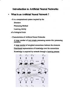
3.3. Obtained results The study of the application of the back-propagation neural network was carried out for a defined data AHP model using the software NeuralWorks Professional II/ PLUS. By alternating, the attributes diverse architectures of neural networks were studied. The attributes of the network that gives minimum RMS error are shown in Table 4. This network architecture generated the network output with 2,27 % rate of RMS error in the learning phase and 7,56 % in the validation phase. Therefore the neural network whose attributes are given in Table 4 approximates best to experimental results. The graphs in Figures 6, 7 and 8 show the results obtained by this network structure with regard to experimental results. The actual classes obtained by the AHP methodology and predicted ones obtained by the trained neural network are shown. Every figure highlights only one class, as well as possible deviations in prediction of appropriate class. From Figures 6, 7 and 8 it is obvious that the neural network acceptable classified items to the classes. Table 4. Attributes of neural network with minimum RMS error Tablica 4. Atributi neuronske mreže s minimalnom RMS grješkom No. / Br.
Accepted denotation / Usvojeno obilježje
Attributes / Atributi
1.
Input number of neurons / Broj ulaznih neurona
4
2.
Output number of neurons / Broj izlaznih neurona
3
3.
Number of hidden neurons / Broj skrivenih neurona
4
4.
Learning rule / Pravilo učenja
Delta / Delta
5.
Transfer function / Prijenosna funkcija
Sigmoid / Sigmoidna
6.
Epoch Size / Veličina epohe
12
7.
Number of iteration / Broj iteracija
50000
8.
Learning Coefficient Ratio / Omjer koeficijenata učenja
0,5
9.
Momentum / Moment
0,4
10.
RMS error in learning phase / RMS grješka u fazi učenja
0,0227
11.
RMS error in validation phase / RMS grješka u fazi validacije
0,0756
12.
Correlation Coefficient / Koeficijent korelacije
0,9831
320
K. ŠIMUNOVIĆ et. al., Application of Artificial Neural Networks...
Strojarstvo 51 (4) 313-321 (2009)
The AHP model as well as the neural network model can be effectively implemented to inventory module of ERP systems. The real new inventory data form ERP system can be used to enlarge the amount of sample data. It is to be expected that after learning and training the network will give better results i.e. smaller error. Further research will be directed to the selection of the reliable supplier for the A classified items and suggestion of the appropriate inventory strategies and policies. Figure 6. Presentation of actual and predicted values given by neural network for inventory class A Slika 6. Prikaz stvarnih i procijenjenih vrijednosti dobivenih neuronskom mrežom za klasu zaliha A
References [1] CUS, F.; ZUPERL, U.: Adaptive self-learning controller design for feedrate maximization of machining process, Advances in Production Engineering & Management, 2 (2007) 1, 18-27. [2] ZUPERL, U.; CUS, F.: Optimization of cutting conditions during cutting by using neural networks, Robotics And Computer-Integrated Manufacturing, 19 (2003) 1-2, 189199. [3] BALIC, J.; KOROSEC, M.: Intelligent tool path generation for milling of free surfaces using neural networks, International Journal of Machine Tools & Manufacture, 42 (2002) 10, 1171-1179.
Figure 7. Presentation of actual and predicted values given by neural network for inventory class B Slika 7. Prikaz stvarnih i procijenjenih vrijednosti dobivenih neuronskom mrežom za klasu zaliha B
[4] SIMUNOVIC, G.; SARIC, T.; LUJIC, R.: Surface quality prediction by artificial neural networks, Technical Gazette 16 (2009) 2, 43-47. [5] BREZAK, D.; UDILJAK, T.; MIHOCI, K.; MAJETIĆ, D., NOVAKOVIĆ, B.; KASAĆ, J.: Tool Wear Monitoring Using Radial Basis Function Neural Network, International Joint Conference on Neural Networks – Proceedings, Budapest, 2004. [6] SIMUNOVIC, G.; SARIC, T.; LUJIC, R.: Application of neural networks in evaluation of technological time, Strojniški vestnik - Journal of Mechanical Engineering, 54 (2008) 3, 179-188. [7] SARIC, T.; LUJIC, R.; SIMUNOVIC, G.: Applying of artificial neural network in maintenance planning of metallurgical equipment, Metalurgija, 44 (2005) 2, 107112.
Figure 8. Presentation of actual and predicted values given by neural network for inventory class C Slika 8. Prikaz stvarnih i procijenjenih vrijednosti dobivenih neuronskom mrežom za klasu zaliha C
4. Conclusion By comparing the results of neural network inventory classification with the original data AHP model, it can be concluded that neural network model predicted classes with acceptable accuracy. RMS error in learning phase amounts to 2,27 % and 7,56 % in the validation phase. It can be seen that the smallest error appeared in classifying items to class C because of the biggest sample data.
[8] PARTOVI, F.Y.; BURTON, J.: Using the analytic hierarchy process for ABC analysis, International Journal of Production and Operations Management, 13 (1993) 9, 29-44. [9] LEI, Q.S.; CHEN, J.; ZHOU, Q.: Multiple criteria inventory classification based on principal components analysis and neural network, Advances in neural networks - Proceedings, Berlin, 2005. [10] CHU, CW.; LIANG, GS.; LIAO, CT.: Controlling inventory by combining ABC analysis and fuzzy classification, Computers and Industrial Engineering, 55 (2008), 841-851. [11] GUVENIR, H.A.; EREL, E.: Multicriteria inventory classification using a genetic algorithm, European Journal of Operational Research, 105 (1998), 29-37.
Strojarstvo 51 (4) 313-321 (2009)
K. ŠIMUNOVIĆ et. al., ������������������������������������������������ Application of Artificial Neural Networks...���� 321
[12] SAATY, T.L.: The analytic hierarchy process, McGraw Hill, New York, 1980. [13] SAATY, T.L.: How to make a decision: the analytical hierarchy process, European Journal of Operational Research, 48 (1990) 1, 9-26. [14] SIMUNOVIC, K.; DRAGANJAC, T.; SIMUNOVIC, G.: Application of different quantitative techniques to inventory classification, Technical Gazette, 15 (2008) 4, 41-47. [15] CHEN, Y.; LI, K.W.; KILGOUR, D.M.; HIPEL, K.W.: A case-based distance model for multiple criteria ABC analysis, Computers and Operations Research, 35 (2008), 776-796. [16] BHATTACHARYA, A.; SARKAR, B.; MUKHERJEE, S.K.: Distance-based consensus method for ABC analysis, International Journal of Production Research, 45 (2007) 15, 3405-3420. [17] FLORES, B.E.; WHYBARK, D.C.: Multiple criteria ABC analysis, International Journal of Operations and Production Management, 6 (1986) 3, 38-46
[18] FLORES, B.E.; WHYBARK, D.C.: Implementing multiple criteria ABC analysis, Journal of Operations Management, 7 (1987) 1, 79-84. [19] RAMANATHAN, R.: ABC inventory classification with multiple-criteria using weighted linear optimization, Computers and Operations Research, 33 (2006), 695700. [20] NG, W.L. A simple classifier for multiple criteria ABC analysis, European Journal of Operational Research, 177 (2007), 344-353. [21] ZHOU, P.; FAN, L.: A note on multi-criteria ABC inventory classification using weighted linear optimization, European Journal of Operational Research, 182 (2007), 1488-1491. [22] MASTERS, T.: Practical Neural Network Recipes in C++, Academic Press, San Diego USA, 1993. [23] PARTOVI, F.Y.; ANANDARAJAN, M.: Classifying inventory using an artificial neural network approach, Computers and Industrial Engineering, 41 (2002), 389404.