Application of Convolutional Neural Networks to Four-Class Motor

260

Information Technology and Control

ITC 2/46 Journal of Information Technology and Control Vol. 46 / No. 2 / 2017 pp. 260-273 DOI 10.5755/j01.itc.46.2.17528 © Kaunas University of Technology

2017/2/46

Application of Convolutional Neural Networks to Four-Class Motor Imagery Classification Problem Received 2017/03/02

Accepted after revision 2017/05/12

http://dx.doi.org/10.5755/j01.itc.46.2.17528

Application of Convolutional Neural Networks to Four-Class Motor Imagery Classification Problem Tomas Uktveris, Vacius Jusas Kaunas University of Technology, Software Engineering Department, Studentu st. 50, Kaunas, Lithuania, e-mail: [email protected], [email protected] Corresponding author: [email protected] In this paper the use of a novel feature extraction method oriented to convolutional neural networks (CNN) is discussed in order to solve four-class motor imagery classification problem. Analysis of viable CNN architectures and their influence on the obtained accuracy for the given task is argued. Furthermore, selection of optimal feature map image dimension, filter sizes and other CNN parameters used for network training is investigated. Methods for generating 2D feature maps from 1D feature vectors are presented for commonly used feature types. Initial results show that CNN can achieve high classification accuracy of 68% for the fourclass motor imagery problem with less complex feature extraction techniques. It is shown that optimal accuracy highly depends on feature map dimensions, filter sizes, epoch count and other tunable factors, therefore various fine-tuning techniques must be employed. Experiments show that simple FFT energy map generation techniques are enough to reach the state of the art classification accuracy for common CNN feature map sizes. This work also confirms that CNNs are able to learn a descriptive set of information needed for optimal electroencephalogram (EEG) signal classification. KEYWORDS: convolutional neural network, motor imagery, feature map, image classification, FFT energy map.

Introduction Motor imagery classification is one of many widespread machine-learning problems of brain-computer interface (BCI) systems. With the need for human mind controlled applications the recording of elec-

troencephalograms (EEG) has emerged as an optimal solution for non-interventional brain activity analysis. The ability to fully understand this brain induced electrical signal would greatly simplify the life for


2017/2/46

people with disabilities or break the barrier for natural interaction in entertainment industry.

short review of the common techniques is presented in the remainder of this section.

This work focuses on four-class motor imagery problem where the recorded EEG signal is classified into four different classes that correspond to four different human subject imagined motoric actions (left hand, right hand, feet and tongue movement). Even if a simpler two-class (binary) problem achieves good classification performance, the four-class still struggles to reach the same results and requires more scientific investigation.

CNN was successfully used by Mirowski et al. [12] to predict epileptic seizures from EEG. The authors have proposed to use four types of bivariate statistical properties of the EEG signal as features for classification. They argue that commonly used univariate features (computed on each EEG channel separately) lack the required channel relationship information. Cross-correlation, non-linear interdependence, Lyapunov exponent and wavelet synchrony feature information was packed into 2D images for classification. Prediction accuracy of 70% was achieved. Another work in the field of EEG analysis was dedicated to solving the SSVEP (Steady State Visually Evoked Potential) signal classification problem by Cecotti and Gräser [6], where a subject is introduced to visual stimulation at a specific frequency. A four layer CNN network topology with a Fourier transform filter in second layer was tested. Selected architecture proved to achieve up to 97% classification accuracy. It was noted that the switch from time domain to frequency domain gave a positive effect on the classification performance. However, introduced reliability rejection criteria for each class made the final solution less robust, produced a lot of sample rejections and gave average generalization. Different application of CNN to the SSVEP is described in a paper by Bevilacqua et al. [2]. The authors used a four layer network architecture with a hidden L2 Fast Fourier Transform (FFT) layer for frequency extraction. Due to the nature of the problem the signal analysis was done in frequency domain. Channels Pz, PO3, PO4, Oz (of 10-20 electrode system) were used to record EEG samples at 256Hz within 2 second windows. Images of 4x512 elements were composed of filtered EEG data and used as input for the CNN classifier. Network was trained for 1000 epochs. Mean accuracy of 88% was obtained by this method.

A relatively new and perspective approach to EEG data classification was found in deep learning branch of machine learning. Convolutional neural network (CNN) is a novel animal visual cortex inspired method for image based classification that has not been widely used with EEG, let alone motor-imagery task. With the abilities to generalize/pool and self-learn the needed features in non-linear ways it can benefit EEG classification. Since EEG motor imagery task lacks accurate solutions the CNN could be the new perspective way to look deeper into the same problem. Regarding its novelty and success in other fields it was chosen as the main tool for four-class EEG motor imagery problem analysis in this paper. By using CNN for classification subtle fine tuning is required to receive best results. This involves selecting a proper neural network architecture, feature method and feature map size. These nuances and their effect on classification performance are further analyzed and discussed in this paper. Furthermore, feature extraction and feature map (image) generation methods for classification are of great significance. In simplest cases, the EEG signal and feature vector can be treated as one-dimensional signal. In order to move to two-dimensional image classification, two dimensional features or feature transformation methods are required. Possible techniques for such a task are presented and discussed in this work.

Related work In recent years, an increasing number of papers that use CNN for EEG classification task have been published. Multiple approaches have been proposed for solving motor imagery and other related problems. A

CNN capability of detecting P300 events from EEG was showcased by Cecotti and Gräser [7] with accuracy of 95%. The signal analysis was conducted separately in time and space domains. Images of 64x64 in size created from 64 channels of downsampled EEG data were used for classification. Seven different CNN models were verified. Additionally, the work employed a strategy to use vector based CNN kernels instead of matrix kernels in order to prevent mixing

261

262


features related to space and time domains. A technique based on trained network first layer weight analysis was used to extract 8 most relevant electrodes for each subject. Recently, CNN has been used by Manor et al. [11] to solve RSVP (Rapid Serial Visual Presentation) task (where a subject has to detect a target image within five possible categories). The authors introduced, a spatio-temporal regularization penalty for EEG classification to reduce network overfitting. Accuracy of 75% was reached with CNN architecture of three layers having 64x1 convolutional, two pooling and two fully connected filters. Images of 64x64 (64 channels by 64 time samples) were used as input for the network. Advantages of using neural network models against manually designed feature extraction algorithms were presented along with criticism for the manual method for unclear and endless possibilities of combining different methods in an efficient way.

2017/2/46

A more recent study by Bai et al. [1] on 4-class motor imagery proposed a novel Wavelet-CSP (Common Spatial Patterns) with ICA-filter method. The EEG artifacts were removed using negative entropy-based ICA. Mean accuracy of 76% was achieved using SVM (Support Vector Machine) classifier. One of the latest works in the field of CNN and 4-class motor imagery is the paper by Yang et al. [21]. The authors proposed a frequency complementary feature map selection (FCMS) method. ACSP (Augmented CSP) feature filtering was used in their work. Two other feature selection methods - random map selection (RMS) and selection of all feature maps (SFM) were analyzed. FCMS was the best performing method due to its ability to limit the ACSP feature redundancy in different frequency bands. The CNN used 5 layer architecture with 5x5 filters (kernels). The work also demonstrated that CNNs are capable of learning discriminant, deep structure features for EEG classification without relying on the handcrafted features. Average classification accuracy achieved was 69%.

Various techniques directly related to the current motor imagery problem have been proposed over the years in literature. Qin and He in [14] describe an analysis of a two-class motor imagery problem. Authors proposed a technique to analyze the EEG in frequency domain. A time-frequency distribution (TFD) images were constructed based on complex Morlet Methods of analysis wavelet decomposition for electrode pairs. The TFDs were subtracted from symmetrical channels to form Convolutional Neural Networks (CNN) weight matrices that were used to compute in weight- Convolutional neural networks are biologically-ined energy for classification. A Laplacian filter was spired variants of MLPs (multi-layer perceptrons). used for signal preprocessing. Average classification They have been successfully used for character recograte of 78% was achieved for this method. Another nition in the past by LeCun et al. [9] and currently have approach based on energy entropy preprocessing gained interest from researchers due to performance and Fisher class separability criteria was proposed in capabilities. CNNs consist of one or more convolu[20] by Xiao et al. Authors analyzed a two-class motor tional layers, with weights of the layer shared across imagery problem in time-frequency domain. Similar the input. Multiple of such layers form a non-linear TFD distributions (spectrograms) were construct- “filter” chain. The convolution is designed to handle ed from EEG short-term Fourier transform (STFT) 2D data, as opposed to other neural networks that opdata. Three different classification methods were erate on 1D vectors. This ability makes the extracted compared. Classification accuracy for the two class features easier to view and interpret. problem was 85%. A more complicated approach for 3-class motor imagery analysis was done by Zhou Feed-forward neural network et al. in [22]. The study proposed a new method to A typical neural network function as presented by Veextract the MRICs (movement related independent daldi and Lenc [17] is defined as: components) and utilized ICA (Independent Component Analysis) spatial distribution patterns for such (1) (1) �(�) = �� (… �� (�� (�� )� �� ) … , �� ) a task. Different ICA filter designs were tested. ICA �� (2) �: ℝ �→ ℝ � � filter design was confirmed to be subject invariant. (2) �: ℝ�� → ℝ� � � �� (2) Classification accuracy of 62% was received. where x 1,…,xk is the where x 1,…,xk is the

�� =


�

�

�� =

�

(2) �: ℝ�� → ℝ� � � �� where x = (x1�� ,…,xk) is the�network � � � � �� layer input (a M×N (2) where x 1,…,x�: k is the →ℝ size image ℝ with K� channels), w = (w1,…,wn) is the vec�� (2) �: ℝof →kparameters. ℝis the where x learned 1,…,x tor is the Convolution

where x

1,…,xk

A 3-dimensional convolution operation with k’ filter count can be expressed as: �� = � �� ,�� ,�

� = � �� ,�� ,� �� ,�� ,� �� = � �� (3) where y�� is the output of the convolution.

��

(3)

(3)

(3)

Pooling

CNN concept of pooling is a form of non-linear down-sampling. Pooling partitions the input image into a�set of� �� non-overlapping rectangles and, for each �� (2) �: ℝ��such → ℝ sub-region, outputs the maximum or average e x 1,…,xk is the value. This � way � it� is possible to reduce the feature size (2) � � �: ℝ�� → ℝ� � �� : ℝ → ℝ � � ��as required and(2)provide transla(and computation) here x 1,…,xk is theinvariance. Pooling function is given by: tion where x 1,…,x k is the �� = �� : � � � � � � + �, � � � � (4) � :+� � �� + �, � � � � �� = �� (4) (4) �� = �� : � � � � � � � +� �, + �� (4) � � + �� ,� �� = � where �� y�� is �the p is padding. ,�� output, (3)

��

�� =

. �� ∑� �� = �� . � �� ∑� �� = � . ∑��

(7) (7) (7)

2017/2/46

,

(6) � � �� + � ∑��(� � ) �� = , (6) � = �� (6) + � ∑��(� � ) �� , meters, G(k)=[k− is a group of ∑ �� + � ⌊ρ2 � ⌋,k+�)⌈�ρ2��⌉]∩{1,2,…,K} ��(�

ρ consecutive feature channels in the input map. Softmax

The operation computes the softmax operator across feature channels and, in a convolutional manner, at all spatial locations. It is a combination of an activation function (exponential) and a normalization operator: �� =

� ��

�� ∑� ��

.

(7)

(7)

� � ��. �� = � (7) ��∑�� = �� . (7) Common Spatial (CSP) ∑��Patterns � ��

CSP is a widely adopted signal pre-processing method that decomposes the raw EEG into subcompo� ��: ∑maximum nents (spatial patterns) ��(� having differences � �) (8) � in variance as shown by Naeem et al. [13]. Wang et(9) al. � (∑ ��(�)� ��: ∑ �) �= � �� : � (8) � + ∑� in [19] concluded that this technique allows better � ��: ��(� ∑� �(∑ �)+ ∑ )� = � (8) (9) �� : � � � thus more acfeature separation in feature space and �� (∑� + ∑Also, � property (9) � )� = curate signal��: classification. the of CSP to decrease feature dimensionality is very suitable for EEG data complexity reduction. It has been shown by Uktveris and Jusas in [16] and other works that this method gives a substantial EEG signal classification performance increase, thus is a highly recommended filtering method.

Non-linear � � ,� �� = � �� gating The filter is a spatial coefficient matrix W: (3) �� = � �� ,�� ,�� ,� (3)linear functions �� Typical CNN non-linear filters use S = WT E �� with a non-linear gating function, applied identical- where S is the filtered signal matrix, E is original ly to each component of a feature map. The simplest EEG signal. Columns of W denote spatial filters, such function is the Rectified Linear Unit (ReLU). while inverse, i.e. W-1, are spatial patterns of EEG (5) �� = ��, �� . Such filter can be written as: signal. The criterion of CSP for a two C1, C2 class (5) �� = ��, �� . � by: problem is given ��: ��(� ∑� �) (8) (5) �� = ��, �� . (5) � (∑ (9) )� �� : � +∑ =� (8) ��:��(�� ∑� �) (8) ��: ��(� � ∑� �) Normalization (8) � (∑ (9) �� : � + ∑ )� = � (9) �� : �� (∑� �+ ∑� )� = � Another important � CNN building block is chan(9) � : � � � � normalization. � + �, � � � �� = �� nel-wise This (4) operator normalizes � vector � + �� over feature channels at each spatial locawhere ∑1 and ∑2 are the class covariance matrices. 3 the �� = �� : � � � � � �� + �, � � � � � � �� = �� : � � � � � + �, � � � tion� �in the input map x. The form of the normaliza(4) � � 3 Solution can be acquired by solving a generalized ei(4) � + �� is: tion � operator � � + �� genvalue problem. Since CSP was designed for a bi3 nary problem, multiclass solutions are combined of �� multiple spatial filters. �� = , (6) � � (6) �� + � ∑��(� � ) �� Due to the broad and positive acknowledgement of where y is the output; κ, α, β are normalization para-

�� = ��, �� .

�� = ��, �� . �� = ��, �� .

(5) (5)

(5)

CSP, the method was used in the current work to filter EEG data before commencing feature extraction.

263

264


Feature extraction methods

Mean window energy (MWE)

A multitude of EEG feature extraction methods have been studied by Uktveris and Jusas in [16] and other literature. Their output usually is a one dimensional feature vector that can be used for classification. The ability to adapt the algorithms for two-dimensional CNN has not been thoroughly analyzed. It is also important to know if the adapted methods can give similar or better results when applied in 2D for CNN. Thus, a review of the most common feature extraction techniques and their implementations for CNN is presented in this work. A short description of the EEG feature methods that were tested and analyzed in this paper is given next. Mean channel energy (MCE) The energy of each i-th EEG channel is computed as the mean of squared time domain samples (10). The result is then transformed using a Box-Cox [4] transformation (i.e. logarithm) in order to make the features more normally distributed, and finally, the resulting values are combined into a feature vector: 1 �

�

� �� = ��1� � �� = 1� �. �� = 1� �� = �� . � ��

(10) (10) (10)

��

� Variance for each i-th EEG channel is the second mo1 � �� = �� about � � � =its 1� �. ment of the signal computed mean . The(10) result � � �� is normalized using Box-Cox for final feature vector: � 1 �� = 1� (10) �� = �� . � 1 1 � � � � �� = �� = 1� � . (11)(11) = ��1�� (�� ) � � � =(10) 1� �. 1 �� (11) �� ) � = �� (� � � � � = 1� � . � � � � � � �� (10) �� = �� = 1� � . � ��

��

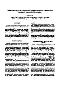
An example of a feature map generated using this � technique is given1 in Figure 1. � �� = �� (�� ) � � � = 1� �. �

�� Figure 1 Feature map generated with CV method

�

��

(11) (11) (11)

This technique computes (12) the mean signal energy of N windows of size W=s/N for each i-th EEG channel (where s is EEG channel sample count). The resulting coefficients are Box-Cox transformed (12) to form final map: ��

�

�

��

��

1 1 = �� = �� 1� � . � �

(12)

The maximum window count in experiments was selected as p=n (where n is EEG channel count) in order to form rectangle feature maps. Principal Component Analysis (PCA) PCA is a filtering technique that decomposes input �� (13) )|� by� using � = |��(� = 1� � orthogonal . signal into main components �� (13) �� =� |��(�� )|�� = 1� �. transformations (13). Wang et al. showed in [18] that it also can be used to suppress artifacts and noise in EEG signal. The decomposition (13) is carried out multiple times – initially to determine the principal � 1 – to suppress � components, secondly noisy compo� �� (14) �� = ��1� � �� = 1� �. � �� nents at decomposition levels 1-3: � � ��= �� = �� (13) (14) �� = �1� � . 1� � . � = |��(� � � )|��

Channel variance (CV)

1 �� = �� (� �� )� � � � = 1� �. � �� 1 � � �� = �� (�� ) � � � = 1� �. 1� �� = �� (� �� )� � � � = 1� �. �

2017/2/46

(11)

�� (13) (13) �� = |��(�� )|� � = 1� �. �� (13) �� = |��(�� )|� � = 1� �. �� The feature vector consists of filtered EEG mean (13) |��(� )| � �� =final � � = 1� � . � 1

�� energy elements via Box(14) �� = �� (14) � that �� were � � � = normalized 1� �. � �� Cox: � 1 �� (14) �� = �� = 1� �. 1 � �� (14) (14) �� = �� = 1� �. 1� � �� (14) �� = �� = 1� � . � �� Multi-resolution of 5 levels with Daubechies’ � 1 (4 vanishing � least-asymmetric wavelet �̅ �� = ��1� � �� moments)(15) � �� (15) �̅ �the �� =decomposition �� was used for in�� this� work. � ��

Mean band power (BP)

�

1 Algorithm �̅calculates power �� = �� the (15) fre� three major � �� of � quency bands: 8-14Hz,��19-24Hz and 24-30Hz (corresponding to Mu, Alfa and � Beta brain waves) by first 1 signal using the 4-th order � band-pass filtering the �� (16) � �� 1= � �̅ �� = 1� �� ̅ �� = 1� � � (FIR) filter. (16) �� = �impulse Butterworth finite 1 � �� response � �� (15) �̅ �� = �� 11 � � � � � �� (15) �̅ �� = �� = � �� (16) 1 � � � �̅ �� = 1� (15) �� ̅ �� = �� (15) � ��

�

1 �� ̅ �� = 1� �� = � � 1 � �� = �� ̅ �� = 1� � 1� �� = �� ̅ �� = 1� � � � ��

(16) (16) (16)

��


�� (�, �) = �

2017/2/46

265

� � �(�) �� (�) =� , � = �,1, � , � �� = l�� (� )� � , � = 1, �.

�

1 � (15) �̅ �� = �� 1�� (18) � � � � � �(�) � � � �(�) � (15) the �̅ � �� = �� The resulting�� signal is then squared to obtain � � , � = �,1, � , � �� (�) = , � = �,1, � , � ��1(�)��=��(�) �(�) (19) �� smoothing (19) �� , � = �� (�) �,1, � , �� power, and a w-sized window �� operation (�) = = = �,1, �� , �� (19) � � (1��, �) � �� 1�� = , � =(1, ln�� (19) � � �� ) � is performed to filter the signal as shown in (15). The �,� (20) � �� 1 �� mean power values (16):1 ��1= �� ln�� (1 � �) � �� 1�� , � = 1, � (20) 1,� �=ln�� (1 � � �) �� 1�� 1�� = �� ,,�� = 1, � �� = � ln�� (1 � �) � �� 1, � (20) (20) �� (1 �� ) � 1�� = ln�� = 1, � � (20) � � � � � � �� =

�

��

1 �� 1�̅ �� = 1� � � �� = �� ̅ �� = 1� � �

(16)

(16)

(16)

��

of each computed band are then used as feature vector components. Channel FFT energy (CFFT)

��

(19)

Channel Discrete Cosine Transform (DCT) Signal energy concentration can be estimated via DCT as shown by Birvinskas et al. in [3]. The sum of squared DCT coefficients of each i-th EEG channel forms the feature vector components of this method (18). Features are normalized using Box-Cox transform: �

�� = l�� (�� )� � , � = 1, �. � �� = l�� (�� ) � , � = 1, �. ��

(18) (18) (18)

�� = |��(�� )|,

Time Domain Parameters (TDP)

1 �� = � � ln�� (1 � �) � �� 1�� , � = 1, � 1 � �� = � ln�� (1 � �) � �� 1�� , � = 1, � � ��

(20) (20)

��,�

�� (�,

here u is the moving average parameter, u ∈ [0; 1].

� 1 �� = Teager-Kaiser Energy Operator (TKEO) � 1 �� = � = � � �(�) ��calculation = �� , �� TKEO is a �more accurate , � =signal �,1, � , energy � � (�) = � � low (19) method that allows �� to detect high frequency and �=1 ��,� ( � amplitude 1 components. Approximation for discrete �� = � ln�� (1 � �) � �� 1�� , � = 1, � (20) i-th EEG �channel signals is given by (21). ��

1

(21) �� =

(22)

1

�

�

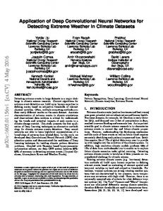
�� (22) l�� (FFTEM) � Ψ�� , � = 1, � �� =map FFT energy � �� Figu This method generates a 2D feature map from EEG by Figure Figure using FFT. Each i-th EEG channel signal is transformed into frequency domain and forms a single row in the feature map as shown in (23). Full signal window was used to gain a global energy view as opposed to the work by Hu Figure 3. Feature map ge et al. [8], which used short-term FFT windows. Figure

�� = |��(�� )|, � = �� 1, � � �� = 1, �� |��(��)| )|,, �� = = |��(� = �� 1,��

(23)(23) (23) (23)

The computed map H is scaled to required feature map size for CNN classification. Figure �� 2 shows an |�� ()|�� )|, with �� = � = 1, � �� |��(� example result map generated this method. = , � = 1, � (23) � �

� = �� 1,Figure � 2

Time domain parameters compute time-varying energy of the first k derivatives of the i-th EEG channel. Obtained derivative values (19) are smoothed using exponential moving average and a logarithm is taken as given by (20). The resulting signal mean is used in feature vector generation. � � �(�) �� (�) =� , � = �,1, � , � (19) � �(�) �� (19) �� (�) = , � = �,1, � , � � (19) ��

�� ((��

(� � = �(20) ��2�� ,�

As analyzed by Cecotti and Gräser in [7], this method employs the Fast Fourier Transform (FFT) for com�� =� � � �� 1�� + 1� (21)�(21) �� = ��1�� ++ �1� � 1��(21) + 1 �� = � puting i-th EEG channel signal energy estimation in �� = �� 1�� 1� (21) 1 � the frequency domain. The FFT result is squared and �� , � = 1, (22) �� = l��11� � � Ψ � 1 the sum of all elements �� = � � �� 1�� + � � ��is��computed: (22) = l�� Ψ � � , � = 1, � �� 1 �� (21) � � (22) �� = l�� Ψ � � , � = 1, � �� l�� Ψ�� , � = 1, � (22) �� = � �� (17) �� = �� (� 1 � ) � � � = 1� � �� )��= ��(17) (22) �� = �� l�� = 1� �� Ψ(17) , � = 1, � �� (�� The components of� the final feature vector are com� �� = � �� 1�� + 1� (21) �� puted by�� using (22). Final feature vector components are formed after Box-Cox transformation is applied.

�( �)

�∞

(23)

FFT energy map example

+∞

�� (�, �) = +∞ � �(�) ��,� (�)�� . �� (�, �) = � �∞ �(�) ��,� (�)�� .

(23)

�� = �� ,

�=

(24) (24)

�∞

�

(��)2

�2��(��) 2 ��,� �(��2� �) = Figure 2. (FFT energy example ��map )2 � Figure 2. FFT energy map example ( ) �2�� 2 Figure 2. FFT energy map example ��,� (�) = �� 2�

� �

�

(25) (25)

Figure 2. FFT energy map example

1

�

�� = �� , �� , 1� �� = �� , �� , �=1

�

�� 5l�� = 1, � .�� =(26) 5 5 �� (26) � = 1, �. 5

� Figure �=1 2. FFT energy map example

,

Figure 3. Feature map generated with CWT

266


Complex Morlet Wavelet Transform (CWT) CWT is a time-frequency analysis method used by Le �� |��(� �� =Van = [10] 1, � for obtaining (23) wavelet coeffi� )|,et al.� in Quyen maps� )| W, (24)� at specific frequencies, that were ��cient = |��(� = �� 1, � (23) analyzed more by Qin and He in [6]:

)

+∞

�� (�, �) = �

18)

9)� . �� 1,

�∞ +∞

(18)

)0)

20)

�

(19)

1)

�� 1, � � , � = (20)

(19) (20)

�=1

�� =

(��)2 �2��(��) � 2�2 � �� +∞

(25)

5

(��)2 2 � (��) ( ) �2�� 2 2 = �� 1, ) 2� �= �2��(�� ,� (�) 2� 5 �� (�) (26) ��,� �� , � �� , � = � . � � � �

1�

(25)

(28)

Figure 4 Feature map generated with SEM

Figure 4. Feature map generated with SEM

(21) (22)


CNN architecture selection Choosing the correct network architecture for the problem gives a greater probability of getting better classification results. CNN supports serially connected layers. Due to the large number of different layer types it is not trivial to find an optimal chain that closely matches the given problem.

�� = 1, �.

(27)


Raw signal (RAW) �� features = �� , � = 1, �.

(27)

RAW is a baseline method that uses the initially pre-processed EEG signal as values for the feature (23) (23)

(28)

(25)

Figure 3.� Feature �� = � = 1, � .map generated with (27) CWT �,

23)

� = �� 1, � .

�=1

�� = �� ,

)

�� = l�� ,

(26)


3)

Signal energy map (SEM)

(25)

Figure 3 Feature map generated with CWT Figure 3. Feature map generated with CWT

(22)

�� = �� , � = 1, �. (27) If necessary, the resulting feature map is scaled to the required image size for CNN training.

In this work, 22 different frequencies were used from �band � along with wavelet cycles from [0; 30] Hz range 1 1 �� (26) �� = �� , , this = range [0.5; 5].�An example output method giv�� = �� , �� , � ��of � =� 1, �1, . � . is(26) � � �� en in Figure 3. �=1 �=1

22)

(21)

(27)

If necessary, the resulting feature map is scaled to the required image size for CNN training. An example map generated with this method is given in Figure 4.

21)

� + 1�

(27)

(24) (�) ��,� (�)�� . = example � �+∞ �� (�, �) Figure 2. FFT� energy map Finally,1 the �� (�, �)�∞ is �decomposed back .to initial 2 (24) )� (�)�� = �((� ) �� ,� �� (26) �� =2.dimensions �� ,map ��2�� (,the ��= 1, �. (25) ) mean �� ∞ � example Figure FFT EEG (�)energy ��,� = ��and � 2�2energy coefficients � � �=1 of each 1 channel form a single row (26) in the feature �� (26) � �� , �� , � = 1, �. � = map: �

)

�� ,�

(24)

�� = 1, �.

This method is using raw EEG signal energy values for feature map generation. The Box-Cox normalized energy of each i-th EEG signal channel is computed and the resulting vector is directly mapped to feature map H i-th row as shown in (28): �� = l�� , � = �� 1, � . (28)

)2)

�� 1, �

(24)

�� = �� ,

(24) (�) ��,� (�)�� . � (�, �) = � �signals All� EEG channel combined as one x(t) signal �∞ are convolved with a number of different frequency Morlet Wavelets+∞ (25), where σ = n/2πf and n is the (24) (�, ((�)�� ) = � �(�) ��,� ��)2 . number of wavelet cycles. � (18) (25) ( ) � 2�2 �∞�2�� ,� (�) = ��

��,� (�) =

) 19)

�(�) ��,� (�)�� .

map. Each i-th EEG signal channel directly maps to feature map H i-th row as shown in (27):

�� =

�� = �� ,

l�� , �� =

�� = l�� ,

� = �� 1, � .

�� ,

�� = 1, �.

�� = 1, �.

� = �� 1, � .

(27)

(28)

(28)

(27)

Tests for 11 different CNN architectures were completed. Starting from simplest and ending with more complex ones. The architecture configurations in a simplified notation are given in Table 1. The used notation is explained in Table 2.

Accuracy

8)

2017/2/46



Notes

1

IC(4)RPFSO

4 filters

2

IC(4)RP(4)FSO

stride 4

3 4. Feature IC(8)RPFSO Figure map generated with SEM 8 filters 4

ICRPFSO

5

IC(32)RPFSO

32 filters

6 Figure 4. IC(64)RPFSO 64 filters Feature map generated with SEM 7

ICRPCRPFSO

8

ICRFSO

9

ICFSO

10

IC(7x1)RC(1x7)RPFSO

Non-rect filters

11

IC(1x7)RPC(7x1)RPFSO

Non-rect filters

Processing time, s

CNN configuration

Accuracy

#

Processing time, s

Figure 5 CNN architecture evaluation

Accuracy

Table 1 Different evaluated CNN architectures

267

2017/2/46

Figure 5. CNN architecture evaluation

Figure 5. CNN architecture evaluation

parameter range scanning approach was carried out to find optimal values.

Table 2 CNN layer symbolic notation Notation

Description (default parameters)

I

input layer of size (44x44x1)

C

convolutional layer (7x7, 16 filters)

R

ReLU layer

P

max pooling layer (2x2, stride 2)

F

fully connected layer (4 classes)

S

softmax layer

O

classification (output) layer

Evaluation results are shown in Figure 5. It can be noted that testing accuracy is around ~65% between most of the configurations. However, training accuracy displays a more dynamic profile from 50% to 80%. In this case, the CNN configuration with the least amount of computational-processing resources (i.e. simplest) should be selected as optimal – 1, 2, 4 or 10.

The momentum value denotes the contribution for the next gradient value from previous iteration in Stochastic Gradient Descent (SGD) method. Larger parameter values decrease the effectiveness of faster learning as shown in Figure 6. In tests, values above 0.6 push the CNN to overfitting and thus decrease generalization and testing accuracy. Value of zero for momentum is not recommended since that invokes a loss of historical gradient learning information. Figure 6 Momentum evaluation

CNN parameter tuning CNNs are more complex since they have more hyper-parameters than a standard MLP. However, the usual learning rates and regularization constants still apply. CNN training parameters, initial learning rate, momentum, batch size and the number of epochs, must be tuned for best performance. Since a 4D parameter grid based search is too resource intensive, a

Figure 6. Momentum evaluation Figure 6. Momentum evaluation

The optimal number of training epochs ensures that the network learns and generalizes the provided features. Excessive epochs deteriorate the testing accu-

Accur

268


racy since the network is overfitting. Figure 7 shows that the optimal count for training is 400-500 epochs. Figure 7 Epoch count evaluation

2017/2/46

bigger Figure than 0.1, testing accuracy 8. while Batch the sizenetwork evaluation peak is achieved with values close to 0.01 as shown in Figure 9. Lower values allow to learn fine grained features, while large ones have the tendency to overfit the network. Figure 9 Initial learning rate evaluation

��ℝ → ℝ� .

Figure 7. Epoch count evaluation size the image count that usedfor forsingle single BatchBatch size is theis image count that is isused

(29) Figu (

��ℝ → ℝ� .

(29)

The first is to interpret the one-dimensional signal as a 2D single row image. However, the negative aspect Figure 10. Feature generated viafilters/ vector duplication of this approach is that only map a single row CNN 7 kernels will be usable.

Accuracy

Accuracy

epoch training. It has direct effect on the network Figure 7. Epoch count evaluation learning quality as shown in Figure 8. The maximum batch size is the number of total images, e.g. N=288 in Batch size is the image count that is used for single experiments. The values lower than N/4 prevent the Feature map generation network from fully maximizing learning efficiency, greater values only increase computational costs at Feature duplication the price of no change in testing accuracy. Many feature extraction methods form a single one-dimensional vector of coefficients known as a Figure 8 feature vector. A problem arises since CNNs are deBatch size evaluation signed to process two-dimensional images. Two approaches for image generation form a viable via solution. Figure 10. Feature map generated vector duplication

The second method, exploiting the CNN translational nature, is to find such a transformation H that allows to convert a 1D signal into 2D:

��ℝ → ℝ� .

Figure 8. Batch size evaluation Figure 7. Epoch count evaluation

Batch size is the image count that is used for single

Figure 8. Batch size evaluation

Initial learning rate must be adopted for each problem. Experiments show that the value should be no

(29)

A simple example for such a transformation is to duplicate the feature vector y in both directions to fill the feature map space. Some additional filtering can be applied to new repeated copies. An example of such feature map is given in Figure 10.

Figure 10. Feature map generated via vector duplication racy

(29)

��ℝ → ℝ� .

(29)


269

2017/2/46

niques are applied. It can be seen that for raw EEG signal analysis nearest filtering method should be used in order to retain original signal details as much as possible. For other feature types the effect could be the opposite.

Figure 10 Feature map generated via vector duplication

Table 3 Raw EEG feature map resize filtering accuracy

��ℝ → ℝ� .

ion

used for single

Filter method

Training

Testing

Nearest

0.47 ± 0.14

0.43 ± 0.11

Bilinear

0.35 ± 0.11

0.33 ± 0.12

0.33 ± 0.10

0.32 ± 0.11

(29)

Figure 10. Feature map generated via vector duplicationBicubic A baseline method and the simplest approach from all feature extraction techniques is to classify the raw EEG signal samples. The raw EEG data form factor of NxM, (where N is number of channels, M is number of samples, N