APPLICATION OF PHYSICS-BASED UNDERWATER ACOUSTIC ...

APPLICATION OF PHYSICS-BASED UNDERWATER ACOUSTIC SIGNAL AND ARRAY-PROCESSING TECHNIQUES TO INFRASOUND-SOURCE LOCALIZATION Gerald L. D'Spain, Michael A. H. Hedlin, John A. Orcutt, William A. Kuperman, Catherine de Groot-Hedlin, Lewis P. Berger, and Galina L. Rovner Scripps Institution of Oceanography Sponsored by Defense Threat Reduction Agency Contract No. DTRA01-00-C-0061 ABSTRACT The purpose of this project is to apply physics-based signal and array processing techniques, recently developed in the area of underwater acoustics, to atmospheric infrasound data and co-located seismic field data. The source of the infrasound data is the newly installed International Monitoring System (IMS) infrasound station at Pinon Flat (PFO). The seismic data are being collected by the Southern California ANZA seismic network. Installation of the eight sensors that comprise the infrasound station at PFO was completed by mid April of this year. The space filters of the array (18 m for the inner centered triangle elements and 70 m for the outer centered triangle elements) also are nearly all in place. Preliminary data collected by this array contain some signals with significant spatial coherence across the array aperture. In particular, a large event with high signalto-noise ratio was recorded on 23 April. Analyses of the arrival structure of this signal are presented in this paper. In addition, the spatial and temporal properties of the background noise in relation to the local environmental conditions are discussed. A focused experiment involving the temporary installation of additional infrasound sensors to provide larger array aperture is being planned for this summer. A description of the planned experiment is presented below. KEY WORDS: IMS, infrasound, localization, ambient noise, spatial coherence, seismic

OBJECTIVE The hypothesis to be tested is that advanced underwater acoustic signal and array processing techniques, with some modifications, can provide more accurate source locations and source signature estimates of low-level events of interest in the enforcement of the Comprehensive Nuclear-Test-Ban Treaty (CTBT) than conventional methods. In addition, the joint use of infrasonic and seismic data from co-located sensor systems has the potential to significantly increase phase identification and source localization capability, and reduce unwanted background noise. Basic research questions to be addressed in this project include: x

What are the effects of range-dependent, heterogeneous, and time-variable media on infrasound propagation and source localization?

x

How can the location of caustics in infrasound be exploited for source localization? Can the location of these caustics be predicted accurately with available environmental data?

x

Can waveguide invariant techniques, which have proven to provide robust and simple approaches to analyses of underwater waveguide propagation, be used effectively with infrasound data?

x

What are the important sources of infrasonic noise and signals in the southern California environment? How will these measurements be translated into other areas of the world?

91 89 19

Form Approved OMB No. 0704-0188

Report Documentation Page

Public reporting burden for the collection of information is estimated to average 1 hour per response, including the time for reviewing instructions, searching existing data sources, gathering and maintaining the data needed, and completing and reviewing the collection of information. Send comments regarding this burden estimate or any other aspect of this collection of information, including suggestions for reducing this burden, to Washington Headquarters Services, Directorate for Information Operations and Reports, 1215 Jefferson Davis Highway, Suite 1204, Arlington VA 22202-4302. Respondents should be aware that notwithstanding any other provision of law, no person shall be subject to a penalty for failing to comply with a collection of information if it does not display a currently valid OMB control number.

1. REPORT DATE

3. DATES COVERED 2. REPORT TYPE

OCT 2001

00-00-2001 to 00-00-2001

4. TITLE AND SUBTITLE

5a. CONTRACT NUMBER

Application Of Physics-Based Underwater Acoustic Signal And Array-Processing Techniques To Infrasound-Source Localization

5b. GRANT NUMBER 5c. PROGRAM ELEMENT NUMBER

6. AUTHOR(S)

5d. PROJECT NUMBER 5e. TASK NUMBER 5f. WORK UNIT NUMBER

7. PERFORMING ORGANIZATION NAME(S) AND ADDRESS(ES)

Scripps Institution of Oceanography,9500 Gillman Dr,LaJolla,CA,92093 9. SPONSORING/MONITORING AGENCY NAME(S) AND ADDRESS(ES)

8. PERFORMING ORGANIZATION REPORT NUMBER 10. SPONSOR/MONITOR’S ACRONYM(S) 11. SPONSOR/MONITOR’S REPORT NUMBER(S)

12. DISTRIBUTION/AVAILABILITY STATEMENT

Approved for public release; distribution unlimited 13. SUPPLEMENTARY NOTES

Proceedings of the 23rd Seismic Research Review: Worldwide Monitoring of Nuclear Explosions held in Jackson Hole, WY on 2-5 of October, 2001. U.S. Government or Federal Rights. 14. ABSTRACT

See Report 15. SUBJECT TERMS 16. SECURITY CLASSIFICATION OF: a. REPORT

b. ABSTRACT

c. THIS PAGE

unclassified

unclassified

unclassified

17. LIMITATION OF ABSTRACT

18. NUMBER OF PAGES

Same as Report (SAR)

10

19a. NAME OF RESPONSIBLE PERSON

Standard Form 298 (Rev. 8-98) Prescribed by ANSI Std Z39-18

x

What acoustic propagation codes (e.g., ones based on a parabolic equation (PE) solution to the acoustic wave equation which includes the effect of winds) incorporate the important propagation physics and so can be used for effective forward modeling in the inverse problems of localizing sources and inferring atmospheric properties?

x

A question related to the inverse problem is how effective are sources of opportunity, e.g., mining and quarry blasts and bolides, in calibrating the atmospheric propagation characteristics?

x

What are the spatial correlation lengths of various infrasound signals and noise at frequencies of interest scientifically and operationally? How do these correlation lengths vary with topography, weather, humidity, background noise, and other environmental variables?

x

How can seismic and acoustic data be used in parallel to understand infrasonic wave excitation and propagation and to localize the source? In particular, how do seismic and acoustic waves couple at the interface between the earth and atmosphere and can this coupling be used to both identify the many wave types observed and infer source location?

RESEARCH ACCOMPLISHED Array Geometry and Description of Data Infrasound data for this project are being collected by the newly installed International Monitoring System (IMS) station at Pinon Flat Observatory (PFO). This station is located in the high desert region 125 km northeast of San Diego, California. It is deployed on land that is part of, and adjacent to, the geophysical observatory operated by the Institute of Geophysics and Planetary Physics, University of California, San Diego (IGPP-UCSD). The PFO lies between the San Andreas and San Jacinto faults, the two most active faults in Southern California. Co-located with the IMS infrasound station is an IRIS (Incorporated Research Institutions for Seismology) 3-component broadband seismic station that is part of the auxiliary seismic network of the IMS. The sensor locations for these two stations are shown in Figure 1. The infrasound station is composed of an array of eight MB2000 microbarometers, plotted with circles. Four of these microbarometers, plotted with the large-diameter circles labeled L1 through L4, are connected to 70-mdiameter space filters and form a centered triangle with nominal 1.4-km spacing. The other four microbarometers, the small-diameter circles labeled H1 through H4, have 18-m-diameter space filters and a 100-200 m spacing. The IRIS 3-component seismic station is plotted with a triangle. Near the end of the installation of the infrasound station at PFO, on 23 April, 2001, (JD 113), a bolide exploded off the west coast of Baja, California (ReVelle, 2001). This event was recorded by nine infrasound stations. The estimated location of the event, obtained by triangulation, was 29.9° N, 133.9° W and its estimated origin time was 06:12:35 GMT (ReVelle, 2001). At this time, only six of the eight infrasound sensors were connected and recording data; no data were being acquired by sensors L3 and L4. The hour's worth of PFO data encompassing this event, starting at 07:30 GMT, 23 April, are the focus of this paper. Figure 2 shows a spectrogram over this 60-min period from sensor H1. The arrivals from the bolide event, traveling over an epicentral distance of about 1700 km, contain broadband energy that exceeds 2 Hz. The spectral peak occurs near 0.3 Hz. The effective group velocity of the first arrivals over the source-to-receiver path is about 290 m/sec, given the reported epicentral distance and origin time. This value is consistent with propagation in the stratospheric waveguide (e.g., D'Spain, Kuperman, Orcutt, and Hedlin, 2000). The event lasts for 15 min or so with the coda evolving to lower frequency with time. The time series from all six recording infrasound sensors over a 6-min period starting before the first arrival are shown in Figure 3. The arrivals are very coherent across the aperture of the array. Note also that wind-generated contamination is quite low during this period of time due to the early morning hour (local PDT is 7 hours behind GMT) of the event's occurrence.

92 90 20

Figure 1. Map showing the geometry of the newly installed IMS infrasound station at Pinon Flat Observatory along with the IRIS 3-component broadband station. The eight microbarometer locations are plotted with circles and labeled L1-L4 (70 meter spaced filters) and H1-H4 (18 meter space filters), and the IRIS station is plotted with a triangle.

Figure 2. 60-minute spectrogram starting at 07:30 GMT, 23 April, 2001, over the 0.05 to 5 Hz band from data collected by microbarometer H1.

Adaptive Frequency/Wavenumber Processing Given the estimated epicentral location of the bolide event, its back azimuth from PFO is 261°, Figure 1 shows that, since L3 and L4 were not yet operational at the time of the event, the resulting 6-element array has very little aperture in the radial direction. Therefore, only rough estimates of the wavenumber content of the bolide arrivals can be expected to be obtained. However, given the high signal-to-noise ratio of the arrivals, some useful results may come from data-adaptive beamforming techniques. This section is devoted to presentation of the preliminary results of applying white-noise-constrained adaptive plane-wave beamforming (Gramann, 1992; Cox, Zeskind, and Owen, 1987) to the arrivals. In the estimate of each data cross-spectral matrix, the time series was divided into consecutive, nonoverlapping, 45-sec segments. An fft length of 128 points was used with a 50 percent overlap, allowing 13 realizations within the 45-sec segment to be averaged in making the estimate. Since a Kaiser-Bessel window with an alpha of 2.5 was used to window the time series prior to the fft, the resulting statistically independent realizations in the estimate is 12.7. Several white-noise-constrained values were used, starting from 10*log(N) where N is the number of array elements (equivalent to conventional beamforming). The value used in the results to be presented is 6 dB down from 10*log(N). The 2-D array frequency/wavenumber processing output is a function four variables, i.e., frequency, time, wavenumber (or slowness), and azimuth. Figure 4 presents a plot of frequency vs wavenumber for a time period at the beginning of the arrival sequence and for an azimuth of 74°, i.e., a back azimuth of 254° which is the direction most of the arriving energy is propagating from (compared to a back azimuth to the estimated location of 261°). The output energy falls along a line passing through the origin with a slope of nearly 330 m/sec. This energy possibly followed ray paths that turn in the stratosphere at 40- to 50-km altitude. The other lines of energy at multiples of approximately 0.04 rad/m are the result of the sidelobe (nearly grating lobe) character of the array response.

93 91 21

Figure 3. Figure 4. Frequency vs wavenumber. The 3-panel plot in Figure 5 shows the adaptive beamforming output as a function of time and phase slowness over a 15-min period starting at 07:48 GMT for the three lowest center frequencies of 0.156 Hz, 0.313 Hz, and 0.469 Hz. The middle panel contains a slight hint of an evolution from lower to higher slowness values (faster to slower phase velocity) over the 8-min period of the main arrival. However, a more significant departure from the expected arrival structure is shown in Fig. 5c where the energy in the 0.469 Hz bin arrives at distinctly smaller slowness values than at lower frequencies. Work is continuing on this phenomenon to understand the physical cause of this effect after verifying that it is not the result of bias associated with the adaptive beamforming process.

(a)

(b)

(c)

Figure 5. The white-noise-constrained adaptive plane wave beamforming output as a function of time and slowness for a fixed azimuth of 74°. The left panel is for a center frequency of 0.156 Hz, the center panel for 0.313 Hz, and the right panel for 0.469 Hz. The 15-min period of the plots starts at 07:48 GMT.

94 92 22

Vector Intensity Vector acoustic intensity techniques can be applied to the analysis of the data collected by the PFO infrasound array. They are most applicable to the study of fields created by the sum of a large number of contributing sources such as the ambient background field. This section describes the preliminary work done in this area. Vector intensity is the magnitude and direction of acoustic energy flux. It equals the product of acoustic pressure and acoustic particle velocity. Two types of acoustic intensity exist in a sound field. The active component measures the net flux of acoustic energy through the medium (i.e., the propagating part), whereas the reactive component is a measure of the energy flow required to support the spatial structure of the field (i.e., the standing wave part). In acoustic waveguides, the reactive component typically is significant only in the cross-waveguide direction; i.e., the direction perpendicular to the boundaries and parallel to the predominant direction of spatial variability of the waveguide properties. In the plane parallel to the waveguide boundaries, e.g., at the earth-air interface in atmospheric acoustics, only the active intensity typically is important. The development of fft-based methods for the estimation of active intensity using data from two closely spaced microphones (e.g., Chung, 1978) led to the rapid growth of vector intensity techniques in air acoustics. The technique originally proposed by Chung (1978) is the one employed here. The component of the vector active intensity in the direction of the separation between the pressure sensors, Ir (Z), is proportional to the imaginary part of the cross spectrum between the time series recorded by the two microphones, i.e.,

(1) The ambient air density is U and 'r is the separation between microphones. The expression above is valid for frequencies such that k'r < 1, where k is the acoustic wavenumber. At the other end of the spectrum, phase and amplitude mismatch between the microphone responses limit the usefulness of this approach. Examination of Figure 1 shows that the separation between H1 and H2 is nearly parallel to the radial direction towards the bolide and the separation between H1 and H4 is nearly transverse to this direction. The distance between H1 and H2 is such that the expression for the active intensity is valid for frequencies less than 0.36 Hz and between H1 and H4, it is valid below 0.48 Hz. Figire 7 shows the amplitude and sign of the active intensity along the line between H1 and H2 (left panel) and between H1 and H4 (right panel). Positive values represent energy flux from H1 to H2, and from H1 to H4, respectively. The spectrograms are plotted only up to the maximum frequency for which Eq. (1) is valid. The bolide arrivals create large flux in the direction from H1 towards H2 and significantly less along the H1-H4 direction, as expected. In fact, the bolide event can be used as a calibration event to correct for phase mismatch between the three microbarometers. The large energy flow around 0.07 Hz is of the same sign and approximately the same amplitude in both plots, indicating flux from the northwest to the southeast.

95 93 23

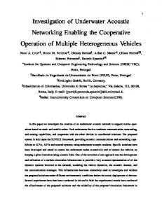
Figure 6. Coherence squared versus frequency and time over the 60-min period starting a 07:30 GMT between microbarometer L2 and two seismometer components of the IRIS station. The left plot is for the vertical component and the right plot is for the east-west component.

Infrasonic/Seismic Coupling The hour's worth of data starting at 07:30 GMT, 23 April (JD 113), were obtained from the IRIS 3-component seismic station at PFO. The location of this sensor system is about half-way between the microbarometer L2 and the remaining cluster of microbarometers about L1, along a line approximately transverse to the direction towards the bolide; refer to Figure 1. As part of the preliminary analysis of these data, coherence squared estimates between each of the microbarometers and the three seismic components over the hour period have been calculated. A sufficient number of statistically independent realizations were included in the estimates so that the true population coherence squared is greater than zero at the 90 percent confidence level if the estimate exceeds 0.21. The minimum value in the two panels in Figure 6 is set to this 90 percent threshold level of 0.21. Figure 6a shows the coherence squared between the time series from microbarometer L2 and the vertical seismometer component time series, and Fig. 6b shows the coherence squared between L2 and the east-west seismometer component. The location of L2 is 328 m from the IRIS station. The coherence squared between the vertical component and L2 is quite high in the 1-3 Hz band at the time of the bolide arrivals. It is also statistically greater than zero between L2 and the east-west component (re Figure 6b) over the 1.5- to 2.5-Hz band at this time. The east-west component is nearly aligned along the radial direction to the bolide source; the coherence squared between L2 and the north-south component show no statistically significant values associated with the bolide arrivals. Surprisingly, the high coherence squared estimates below 0.5 Hz in both panels, probably associated with microseism/microbarom energy, disappears at the time of arrival of the bolide signals. The coherence squared estimates for the bolide arrivals in Figure 6a are higher than for any other seismometer/microbarometer pair. However, those between the vertical component and all other microbarometers still are statistically greater than zero. In contrast, no statistically significant coherence for the bolide arrivals occurred between the horizontal seismometer components and the microbarometers other than the pair shown in Fig. 6b. Also, the coherence between the vertical and east-west seismometer components is significant, but the values for the other two seismometer pairs involving the north-south component are not.

96 94 24

Figure 7. The amplitude and sign of the active intensity as a function of frequency and time over the 60-min period starting at 07:30 GMT, 23 April. The frequency band extends up to the maximum limit of the validity of Eq. (1) in the text. The left plot is for the active intensity component along the line between H1 and H2, and the right plot is the active intensity along the line between H1 and H4.

Relative Dispersion Ranging One of the approaches that will be studied with the data to be collected in a focused experiment at PFO is the estimation of the range to a broadband source using the relative change in arrival times of multipath arrivals along the propagation path. The ideas behind this technique now will be described. The extremely limited aperture of the partially installed PFO infrasound array in the direction along the propagation path prevent this technique from being applied to the data from the bolide event. The concept of using relative dispersion across an array aperture to obtain an estimate of source range can be illustrated with a simple model of a source impulse in time that excites two wave types with different group velocities. Assuming initially that each wave type is non-dispersive and arrives with identical amplitude, A, then the received signal at range r can be modeled as an even impulse pair:

(2) The quantity, tc(r)=rSg , is the average of the times of arrival of the two pulses, where Sg is the average group velocity of the two pulses. The quantity, W(r), the time difference between the two arrivals, is equal to: W(r) = r'Sg

(3)

and 'Sg is the difference in group slownesses. The range to the source can be estimated from Eq. (3), given that prior knowledge of the environment (i.e., the difference in group slownesses) is available, as done in estimating the range to an earthquake by matching travel time curves to seismograms. In ocean acoustics, this approach recently has been applied to single element spectrograms from very long range propagation experiments (Kuperman, D'Spain, Heaney, 2001). At range r+'r, the time delay between the two pulses, W+'W can be determined by applying Eq. (3). Combining the two equations to eliminate 'Sg (assuming it remains constant over 'r)gives:

97 95 25

This equation shows that measurement of the change in arrival times of the two pulses, 'W, between two receivers can be used to obtain source range information without apparently requiring a priori environmental information. That is, using the evolution with range of the received signal properties in Eq. (4) requires less environmental information than using the properties of the signal at a single point. The actual source range is not estimated, but rather a combination of source range and source bearing since the quantity, 'r is, determined by the separation between the two receivers, q, and the direction towards the source, T, i.e., 'r = q cos (T). Similarly, this information can be obtained in the frequency domain, i.e., the Fourier transform of the received signal in Eq. (2) yields

(5)

The phase terms in this expression are of two types, an imaginary term containing the average of the pulse travel times, tc, and a second phase term involving W, the received signal duration. Complex phase terms, arising from delays/advances in the time domain (re the shift theorem in Fourier analysis), are lost in the calculation of the autospectrum:

(6) However, the term involving the difference in travel times, W, is retained. Simulations of the spectra in the range/frequency plane for this simple two-pulse model display a set of striations that tend from higher to lower frequencies as the source/receiver range increases. The condition for following along one of these striations, i.e., keeping the phase term in Eq. (6), ) { W(r)Z/2, stationary, is:

(7)

resulting in:

(8) Therefore, the behavior of the striation pattern in the range/frequency plane contains the same information on source location as the changes in pulse spreading in the time domain, as would be expected from the similarity theorem in Fourier analysis. This information is available by phase incoherent processing since it is obtainable from the spectra of the received signals rather than just their Fourier transforms. The negative sign in Eq. (8) indicates that the frequency content of the striations evolves to lower frequency with increasing range. The two-pulse model can be extended to a set of N pulses each traveling with its own group velocity. Simulations show that, although the widths and relative amplitudes of the individual striations change, the slopes of the striations in the range/frequency plane in this extended case remain unchanged. The reason is that the relative spreading/compression of the arriving signal with change in range remains the same. For source time functions, s(t), that are finite in duration, the received signal is a convolution of s(t) with Eq. (2), and the resulting autospectrum is the product of the autospectrum of s(t) with Eq. (6). Therefore, the results just presented are still valid as long as the character of the source autospectrum (e.g., its bandwidth and the

98 96 26

smoothness of its variation with frequency) allows the striation pattern in the received spectra to remain visible. This requirement is equivalent to requiring that the doublet arrival structure still be visible in the time domain so that both 'W and W in Eq. (4) can be measured. The constant in Eq. (8) relating a fractional change in frequency of the striation pattern to a fractional change in range is -1. This value is a consequence of the fact that the group velocities of the two pulses were assumed to be independent of range and frequency. However, in those cases where the pulses are dispersive so that the time difference between their arrivals is dependent upon frequency as well as range, then application of stationary phase gives

(9) Information on the environment, as represented by the term in brackets in Eq. (9) that measures the change in signal spreading (duration) with frequency, now is required to obtain the source range information. The term in brackets is a constant, 1+J independent of W and Z given that

= J.

The solution to this differential equation indicates that the required functional dependence of WZ with Z is of the form ZJ . From Eq. (3), the fractional change of W with frequency is the same as the fractional change in 'Sg with frequency. D'Spain and Kuperman (1999) show that 'Sg is proportional to frequency raised to the – (1+1/E) power, where 1/E is the waveguide invariant. Therefore,

(10) Plugging this result into Eq. (9) gives the expression for the range/frequency dependence of striation patterns in single element spectrograms (Brekhovskikh and Lysanov, 1982; D'Spain and Kuperman, 1999). In summary, the information on source range obtained from temporal broadening (or compression) of a multicomponent arrival as range increases is equivalent to that obtained by examination of the striation pattern of the corresponding autospectra in the range/frequency plane. The behavior of the striation pattern is derived by a stationary phase analysis of the appropriate phase term. The relevant information is extractable by phase incoherent processing. If phase coherent processing between stations also can be done, then range and bearing can be estimated with data from just two stations. CONCLUSIONS AND RECOMMENDATIONS The 23 April, 2001, bolide over the northeast Pacific Ocean has provided an interesting event for a first look at the data from the newly installed IMS infrasound station at PFO. The effective group velocity and the predominant phase velocity across the array aperture determined by white-noise-constrained adaptive beamforming techniques is consistent with propagation in the stratospheric waveguide. However, the array aperture along the direction towards the source was limited because two of the eight microbarometers, both part of the outer centered triangle, did not record the event. Phase identification and source localization will certainly be aided by data from these sensors in future events. In particular, a formulation for estimating the range to an impulsive event using relative dispersion across the array aperture is presented, but cannot be effectively applied to the 23 April PFO recordings because of this limitation in aperture. Vector intensity techniques can be used with the PFO data at frequencies below 0.3 Hz and show net energy flux from the bolide event in the expected direction. Finally, the bolide arrivals create statistically significant coherence between the vertical component of the IRIS seismic station at PFO (an auxiliary IMS seismic station) and each of the six recording infrasound sensors. This coherence exists even though the IRIS station is over 300 m from the nearest microbarometer.

99 97 27

Preparations for a 2-week focused experiment in September 2001 at the Pinon Flat Observatory presently are underway. Four MB2000 infrasound sensors with space filters will be installed temporarily at four ANZA seismic station sites to create large horizontal aperture. These temporary installations will take place the first week of September with continuous data recording beginning by the 10th of September. This recording period was selected to encompass four planned rocket launches from Vandenberg Air Force Base; 2 Minuteman III launches, a Delta II rocket, and a Titan IV B launch. These events will provide known infrasound signals for focused study (e.g., McLaughlin, Gault, and Brown, 2000). REFERENCES Brekhovskikh, L. M. and Y. P. Lysanov (1991), Fundamentals of Ocean Acoustics, 2nd ed.New York: Springer-Verlag, 140-145. Chung, J. Y. (1978), Cross-spectral method of measuring acoustic intensity without error caused by instrument phase mismatch, J.Acoust. Soc. Am. 64, 6, 1613-1616. Cox, H., R. M. Zeskind, and M. M. Owen (1987), Robust Adaptive Beamforming, IEEE Transactions of Acoustics, Speech and Signal Processing ASSP-35 (10). D'Spain, G. L., W. A. Kuperman, J. A. Orcutt, and M. A. H. Hedlin (2000), Long Range Localization of Impulsive Sources in the Atmosphere and Ocean from Focus Regions in Single Element Spectrograms, Proc. of 22nd Annual Seismic Research Symposium: Technol. for Monitoring the Comprehensive Nuclear-Test-Ban Treaty. D'Spain, G. L. and W. A. Kuperman (1999), Application of Waveguide Invariants to Analysis of Spectrograms from Shallow Water Environments that Vary in Range and Azimuth, J. Acoust. Soc. Am. 106, 5, 2454-2468. Gramann, R. A. (1992), ABF Algorithms Implemented at ARL-UT,ARL Tech. Letter ARL-TL-EV-92-31, Applied Research Laboratories, The University of Texas at Austin, Austin, TX. Kuperman, W. A., G. L. D'Spain, and K. D. Heaney (2001), Long Range Source Localization from Single Hydrophone Spectrograms, J. Acoust. Soc. Am. 109, 5 pt. 1, 1935-1943. McLaughlin, K. L., A. Gault, and D. J. Brown (2000),Infrasound Detection of Rocket Launches, Proc. of 22nd Annual Seismic Research Symposium: Technol. for Monitoring the Comprehensive Nuclear Test-Ban Treaty, 219-230. ReVelle, D. O. (2001), Global Infrasonic Monitoring of Large Meteoroids, J. Acoust. Soc. Am., 109, 5, 2371.

100 98 28