Apr 25, 2016 - Sciences Babu Banarasi Das University Faizabad Road, Lucknow 226028, Uttar ..... The Possible solution is using desert areas where having very stale ...... [102] A. TSINOBER AND H.K. MOFFATT, eds., Topological fluid ...
Manuscript Number: AMC-D-15-02505R1. Title: A note on some recent fixed point results for cyclic contractions in b-metric spaces and an application to integral ...
Math 430-001 (Ellis). Applied Algebra. Fall 2006. Time. Location. Lecture MW 1:
50-3:05pm Eng. 1 Bld. 027. Instructor: Robert Ellis, Assistant Professor of ...
Theory of Charges-(Pure and Applied Mathematics). 1. Algebraic Topology. I. Title 11. Bhaskara Rao, M. 111. Series. 514' 2 QA612. ISBN 0-12-095780-9.
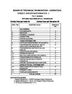
Applied Mathematics -I By W.R Neelakanta Sapna Publications. 2. Applied
Mathematics -I By Dr. ... S Chand Publications. 3. Text book of mathematics for
P U C ...
The Applied Mathematics group in the School of Mathematics at the University of. Manchester ... such as Mathematics in the Life Sciences, Uncertainty Quantification & Data .... used in the modelling of a wide range of physical, biological, engineerin
Reviews of books in areas related to computational mathematics are also ...
Steffen Börm and Stefan A. Sauter, BEM with linear complexity for the ..... AMS
website, corrections may be made to the paper by submitting a traditional ....
ERNST HAIRER
PRELIMINARY DEGREE CHECK. MAJOR in APPLIED MATHEMATICS (MA27).
Name: Admit quarter: PID: Graduating Quarter: Major GPA: Lower-Division ...
Corresponding author R. TALEBITOOTI, E-mail: [email protected] .... defined for each wave component. ... For a two-dimensional problem shown in the x-y plane in Fig. .... in which Ï(l) is the mass density of the lth layer of the shell per unit mids
Apr 25, 2017 - Applied Mathematics and Nonlinear Sciences http://journals.up4sciences.org. QSPR Analysis of Certain Graph Theocratical Matrices and Their ...
Jul 30, 2018 - Applied Mathematics and Nonlinear Sciences 3(2) (2018) 419â426 ... School of Mechanical and Electronic Engineering, Wuhan University of ... A cycle of G is called Hamiltonian cycle if its length is |V(G)|. ...... [12] S. Sudhakar, S.
14 This is the case of "free flow"; see A. H. Gibson, Hydraulics, and its applications,. 4th ed., London ... proaches its maximum cross-section Ac, in a tunnel of cross-section. A0. The rate of ...... earlier work, see A. Eula, l'Aerotecnica (1940).
May 16, 2017 - Applied Mathematics and Nonlinear Sciences http://journals.up4sciences.org. Operations of Nanostructures via SDD, ABC4 and GA5 indices.
Pure and Applied Mathematics Letters 2(2014)1-6. Fixed point theorem applied to a fractional boundary value problem. Assia Guezane-Lakoud. 1. , Allaberen ...
College of Water Conservancy and Hydropower Engineering, Hohai University, ... 2. School of Mathematics and Physics, University of Science and Technology Beijing, ...... olar fluid flow and heat transfer between two porous discs. ... [41] Rees, D. A.
Pure and Applied Mathematics Letters 1(2013)25-33. A characterization of weak statistical convergence via lacunary sequences and ideals. Meenakshi1, M. S. ...
Oct 30, 2014 - Pure and Applied Mathematics Letters, Volume 2015, pages 1-7 ... 1Department of Mathematics, Faculty of Arts and Sciences, Ordu University, ...
CHAPMAN & HALL/CRC APPLIED MATHEMATICS. AND NONLINEAR ... Chapman & Hall/CRC is an imprint of the ... 4.2 Simulation method of Lloyd. 91.
the SPN21 system, they have to be aware of and adaptable to the current method of ... most of them are inclined to use calculators to calculate simple addition, ... on percentages by using the students' prior knowledge on addition, subtraction and ..
More specifically, in Australia, the Great River Murray that passes through New
South Wales, Victoria and ... things) for their mathematical model of the neuron.
Aug 29, 2007 ... for Physicists, 6th ed. ... is: Schutz: Geometrical Methods of Mathematical Physics,
to be ... Pn(x) = 1. 2nn! dn dxn. (x2 − 1)n. (1.7). Generating function: g(t, x) = .... is
the other independent solution of the same differential
Existence and the contact condition. 49. 2.5. The Euler-Lagrange equation. 53 ... We start with a short primer on constrained energy minimization .... The previous example gives a good picture of the mathematical set- .... J(u) = (m + ∫ u, m −∫ u) ≥
i. Finite Difference and Pseudospectral Methods applied to the Shallow Water
Equations in Spherical Coordinates by. DAVID WARREN MERRILL. B.A., Bates ...
Sep 24, 2005 - Computational Methods For Solving Fully Fuzzy Linear .... Gaussian elimination, LU decomposition method and linear programming for finding.
Sunday , September 25, 2005
Computational Methods For Solving Fully Fuzzy Linear Systems ∗
Behnam Hashemi
†
Mehdi Ghatee
‡
py
Mehdi Dehghan
Co
Department of Applied Mathematics, Faculty of Mathematics and Computer Sciences, Amirkabir University of Technology, No.424, Hafez Ave., Tehran, Iran 24 September 2005
Abstract
Re
vi e
w
Since many real-world engineering systems are too complex to be define in precise terms, imprecision is often involved in any engineering design process. Fuzzy systems have an essential role in this fuzzy modelling, which can formulate uncertainty in actual environment. In addition, this is an important sub-process in determining inverse, eigenvalue and some other useful matrix computations, too. One of the most practicable subjects in recent studies is based on LR fuzzy numbers, which are defined and used by Dubois and Prade with some useful and easy approximation arithmetic operators on them. Recently Dehghan et al. [3] extended some matrix computations on fuzzy matrices, where a fuzzy matrix appears as a rectangular array of fuzzy numbers. In continuation to our previous work, we focus on fuzzy systems in this paper. It is proved that finding all of the real solution which satisfy in a system with interval coefficients is NP-hard. The same result can similarly be derived for fuzzy systems. So we employ some heuristics based methods on Dubois and Prade’s approach, finding some positive ex e which satisfies A e=e fuzzy vector x b, where Ae and eb are a fuzzy matrix and a fuzzy vector respectively. We propose some new methods to solve this system comparable to the well known methods such as the Cramer’s rule, Gaussian elimination, LU decomposition method (Doolittle algorithm) and its simplification. Finally we extend a new method employing Linear Programming (LP) for solving square and non-square (over-determined) fuzzy systems. Some numerical examples clarify the ability of our heuristics. Keywords: LR Fuzzy Number, Fuzzy Approximate Arithmetic, Fully Fuzzy Linear System (FFLS), Over-Determined Fuzzy Linear System of Equations, Cramer’s Rule, Gaussian Elimination, Fuzzy LU Decomposition, Doolittle Algorithm, Linear Programming (LP).
One major application of fuzzy number arithmetic is treating linear systems whose parameters are all or partially represented by fuzzy numbers. The term fuzzy matrix, which is the most important concept in this paper, has various meanings. For definition of a fuzzy matrix we follow the definition of Dubois and Prade in [8] i.e. a matrix with fuzzy numbers as its elements [3, 7, 8]. This class of fuzzy matrices consist of applicable matrices, which can model uncertain aspects and the works on them are too limited. Some of the most interesting works on this matrices can be seen in [2, 8]. We limit our attention on this type of fuzzy matrix and employ Dubois and Prade arithmetic operators as mentioned in [3, 8, 10, 11, 19]. A general model for solving a fuzzy linear system whose coefficient matrix is crisp and the right-hand side column is an arbitrary fuzzy vector was first proposed by Friedman et al.[9]. They used the embedding method and replaced the original fuzzy linear system by a crisp linear system and then solved it. In continuation to these works, Dehghan et al. [4] extended some iterative methods on the same system. Here we discuss the case in which all parameters in a fuzzy linear system be fuzzy numbers, which we call it a Fully Fuzzy Linear System (FFLS). We are willing to discuss on the solution of this kind of fuzzy linear systems. Dubois and Prade in [7] investigated two definitions of a system of fuzzy linear equations, consist of system of tolerance constraints and system of approximate equalities. The simplest method for solving this system is creating scenarios for the fuzzy system, which is a realization of fuzzy systems, finding their solutions. Finally we can insert all of the solutions in a set which can be named as the set of solutions, i.e. from fuzzy matrix Ae and fuzzy vector eb, two real matrix and the vector A and b (associate with two positive membership degrees) can be extracted. More over if A be invertible, then vector x = A−1 b with a positive membership, is a solution of this system and {x|x = A−1 b, A ∈ Ae , b ∈ eb } is the set of its solution. Based on these actual scenarios, Buckley et al. [2] extended several methods for this category and proved their equivalence. But their approaches are not practicable, because infinite number of scenarios must be driven from a FFLS. As noticed by Rao and Chen [17], although several investigations have been reported in the literature on the solution of fuzzy systems (Buckley [2], Gvozdik [12], Zhao and Govind [23], and Kawaguchi and Da-Te [15]), very few methods are available for the practical solution of a fuzzy linear system. The main reason of this drawback is in their structure. With more clear statement, as mentioned by Kreinovich et al. [16] finding solution of a system with interval coefficient is NP-hard, i.e. no one has been able to develop any efficient algorithm which requires a number of operations that is polynomial in the size of the input data for solving these problems. They also showed obtaining polynomial algorithm for finding a bound for the solution is hard too. Based on their important results, it is trivial that obtaining the same solution of a FFLS is not easy, because the set of positive fuzzy numbers with neither multiplication nor addition operators has not group structure [8]. In this paper we discuss on this kind of fuzzy linear systems, i.e. we want to solve, A˜ ⊗ x˜ = ˜b, ˜ x˜ and ˜b are fuzzy matrix and vectors with appropriate size. Rao and Chen in [17], where A, provided a computational method to solve this problem, based on their cuts. But presenting a computational method for solving a FFLS using Zadeh’s extension principle, see e.g. [2]. Since there is no analytic formula for some arithmetic operators, Doubois and Prade [8] 2
Elsevier
2 of 21
Sunday , September 25, 2005
2 2.1
Co
py
have extended some approximations for them on a special and useful case of fuzzy numbers, which are used by other researchers [10, 11, 18, 19, 3]. We use these terminology in this work and employ some heuristics based on classic methods from linear algebra such as Cramer’s rule, Gaussian elimination, LU decomposition method and linear programming for finding the approximated solutions of a FFLS. More over, we showed the ability of our approach for solving square and non-square (over-determined) fuzzy systems. The rest of paper is organized as following: Some basic definitions and results on fuzzy numbers are reviewed in next section. Then some approximate operators and definition of a fuzzy matrix, FFLS and its solutions are mentioned. In Section 3 our first method for solving a FFLS is expressed. Then we represent Cramer’s rule for solving a FFLS in Section 4. Factorization methods consist of Gaussian elimination and LU decomposition are introduced for solving FFLS in Section 5. The last method introduced in this paper is based on linear programming approach. Each Section contains numerical examples that describe the efficiency of each method. Section 7 ends this paper with a conclusion and future works.
Preliminaries Fuzzy Numbers
vi e
w
Fuzzy numbers are one way to describe the vagueness and lack of precision of data. The theory of fuzzy numbers is based on the theory of fuzzy sets which was introduced in 1965 by Zadeh [22]. The concept of a fuzzy number was first used by Nahmias in the United States and by Dubois and Prade in France in the late 1970’s. Our definition of a fuzzy number is explained in the following. Firstly we need some other basic definitions, such as fuzzy set. In general a fuzzy set initiated by Zadeh(1965) is defined as follows: Definition 2.1 (Fuzzy Set) Let X denote a universal set. Then a fuzzy subset Ae of X is defined by its membership function µAe : X → [0, 1],
Re
which assigns to each element x ∈ X a real number µAe(x) in the interval [0, 1], where the e value of µAe(x) at x represents the grade of membership of x in A. A fuzzy subset Ae can be characterized as a set of ordered pairs of element x and grade µAe(x) and is often written Ae = {(x, µAe(x))|x ∈ X}.
The class of fuzzy sets on X is denoted with F(X). Definition 2.2 (α−level set) e for which the degree of The α−level set of a fuzzy set Ae is defined as an ordinary set [A] α its membership function exceeds the level α : e = {x|µ (x) ≥ α, α ∈ [0, 1]}. [A] α e A
3
Elsevier
3 of 21
Sunday , September 25, 2005
Definition 2.3 (Extension Principle) Let f : X → Y be a mapping from a set X to set Y . Then the extension principle allows us to define the fuzzy set Be in Y induced by the fuzzy set Ae in X through f as follows: Be = {(y, µBe (y))|y = f (x), x ∈ X}, with µBe (y) = µf (A) e (y) =
supy=f (x) µAe(x), f −1 (y) 6= φ, 0, f −1 (y) = φ,
py
(
where f −1 (y) is the inverse image of y.
Co
Definition 2.4 (Convex fuzzy set) A fuzzy set Ae in X = Rn is said to be a convex fuzzy set if and only if its α−level sets are convex. Definition 2.5 (Normal fuzzy set) A fuzzy set Ae in X is said to be normal if there exist x ∈ X such that µAe(x) = 1. Definition 2.6 (Fuzzy number) A fuzzy number is a convex normalized fuzzy set of the real line R1 whose membership function is piecewise continuous.
w
Definition 2.7 (Positive fuzzy number) A fuzzy number M is called positive (negative), denoted by M > 0 (M < 0), if its membership function µM (x) satisfies µM (x) = 0, ∀x < 0 (∀x > 0).
vi e
Remark 2.8 A fuzzy number could be neither positive, nor negative. Let M and N be two fuzzy numbers with the membership functions µM (x) and µN (x), respectively. Then according to the extension principle of Zadeh, the binary operation ”.” in Rn can be extended to the binary operation of fuzzy numbers M and N in the following form: µM N (z) = sup min(µM (x), µN (y)), z=x.y
Re
To get fast computational formulas for the operations of fuzzy numbers, Dubois and Prade (1987) [6] introduced the concept of LR fuzzy numbers. Definition 2.9 (LR fuzzy numbers) A fuzzy number M is said to be an LR fuzzy number if (
µM (x) =
), x ≤ m, α > 0, L( m−x α R( x−m ), x ≥ m, β > 0, β
where m is the mean value of M and α and β are left and right spreads, respectively, and a function L(.) the left shape function satisfying: (1) L(x)=L(-x). 4
Elsevier
4 of 21
Sunday , September 25, 2005
(2) L(0)=1 and L(1)=0. (3) L(x) is non-increasing on [0, ∞). Naturally, a right shape function R(.) is similarly defined as L(.). Using its mean value and left and right spreads, and shape functions, such a LR fuzzy number M is symbolically written M = (m, α, β)LR .
py
Clearly, M = (m, α, β)LR be positive, if and only if, m − α > 0, (note that L(1)=0.) As examples of typical shape functions, consider the following well-known functions: L(x) = max(0, 1 − |x|P ),
L(x) =
1 , 1 + |x|P
P > 0, P > 0.
Co
L(x) = exp(−|x|P ),
P > 0,
If L(x) and R(x) be linear functions, then the corresponding LR number is said to be a triangular fuzzy number. Definition 2.10 (Equality in fuzzy numbers) Two LR fuzzy numbers M = (m, α, β)LR and N = (n, γ, δ)LR are said to be equal, if and only if m = n, α = γ and β = δ.
w
Definition 2.11 (Subset of a fuzzy number) Since each fuzzy number is a set, we can define its subset as follows. A LR fuzzy numbers M = (m, α, β)LR is said to be a subset of the LR fuzzy number N = (n, γ, δ)LR , if and only if m − α ≥ n − γ and m + β ≤ n + δ.
• Addition (1)
vi e
Concerning the basic operations of such LR fuzzy numbers Dubois and Prade showed exact formulas for ⊕ and together with the approximate formulas for ⊗ and [8]. For two LR fuzzy numbers M = (m, α, β)LR and N = (n, γ, δ)LR the formula for the extended addition becomes:
This formula can be shown as follows. ) = ω = L( n−y ) then x = m − αL−1 (ω) , y = For any fixed ω ∈ [0, 1], let L( m−x α γ n − γL−1 (ω). This implies z = x + y = m + n − (α + γ)L−1 (ω), hence it holds that L( m+n−z ) = ω. α+γ In the same way, for R(ω), it follows that R(
z − (m + n) ) = ω. β+δ
Thus, the formula for the extended addition is proved. For a LR fuzzy number M = (m, α, β)LR and for a RL fuzzy number N = (n, γ, δ)RL the following formulas for the extended opposite and subtraction hold.
5
Elsevier
5 of 21
Sunday , September 25, 2005
• Opposite (2)
−M = −(m, α, β)LR = (−m, β, α)RL .
(3)
py
• Subtraction Let M = (m, α, β)LR and N = (n, γ, δ)RL be two LR and RL fuzzy numbers, respectively.
M N = (m, α, β)LR (n, γ, δ)RL = (m − n, α + δ, β + γ)LR .
Co
• Multiplication M ⊗N A proof similar to the one used for the extended addition of two fuzzy numbers shows that the following formula for the extended multiplication of two positive fuzzy numbers M > 0 and N > 0 holds: z = x.y = mn − (mγ + nα)L−1 (ω) + αγ(L−1 (ω))2 .
w
Here if we assume that α and γ are small enough in comparison with m and n, we can neglect the term αγ(L−1 (ω))2 . By making a similar assumption for R−1 (ω) we can also obtain the approximate formula for the multiplication of two positive fuzzy numbers. When M < 0 and N > 0 or M < 0 and N < 0, it is easy to get similar formulas for their multiplication. Thus, the approximate formulas for the extended multiplication of two symmetric fuzzy numbers can be summarized as follows: if M > 0 and N > 0 then (m, α, β)LR ⊗ (n, γ, δ)LR ∼ = (mn, mγ + nα, mδ + nβ)LR .
See e.g. Dubois and Prade [8], or Giachetti and Young [10, 11].
• Scalar multiplication (7)
λ ⊗ M = λ ⊗ (m, α, β)LR
(
(λm, λα, λβ)LR , λ > 0, (λm, −λβ, −λα)RL , λ < 0.
6
Elsevier
6 of 21
Sunday , September 25, 2005
• Inverse: M −1 Although M −1 is neither a LR nor a RL fuzzy number, because
1−mx αx
∼ =
1 −x m α m2
in the
neighborhood of m1 , the inverse of a fuzzy number M becomes approximately an RL fuzzy number and can be approximated by the following formula: −1 −2 −2 ∼ (m, α, β)−1 LR = (m , βm , αm )RL .
(8)
py
• Division: M N Observing that M N = M ⊗N −1 , the following approximate formula for the extended division of two positive LR and RL fuzzy numbers can be obtained. If M > 0 and N > 0, then
Similar approximate formulas hold when M < 0 and N > 0 or M < 0 and N < 0.
2.2
Fuzzy Matrix
w
Definition 2.12 A matrix Ae = (afij ) is called a fuzzy matrix, if each element of Ae is a fuzzy number [7, 8, 13, 14]. Ae will be positive (negative) and denoted by Ae > 0 (Ae < 0) if each element of Ae be positive(negative). Similarly nonnegative and non-positive fuzzy matrices will be defined.
vi e
Up to rest of this paper, we use positive LR fuzzy numbers and formula 4, in place of exact ⊗. We may represent n × m fuzzy matrix Ae = (afij )n×m , that afij = (aij , αij , βij )LR , with new notation Ae = (A, M, N ), where A = (aij ), M = (αij ) and N = (βij ) are three n × m crisp matrices. Definition 2.13 A square fuzzy matrix Ae = (afij ) will be an upper triangular fuzzy matrix, if afij = 0e = (0, 0, 0),
∀i > j.
Re
The transpose of an upper triangular fuzzy matrix, is lower triangular; that is afij = 0e = (0, 0, 0),
∀i < j.
Definition 2.14 Let Ae = (afij ) and Be = (bf ij ) be two m × n and n × p fuzzy matrices. We e e e f define A ⊗ B = C = (cij ) which is the m × p matrix where cf ij =
L X
afik ⊗ bf kj .
k=1,...,n
7
Elsevier
7 of 21
Sunday , September 25, 2005
2.3
FFLS And Its Solutions
Definition 2.15 Consider the n × n linear system of equations:
.. . (a g f1 ) ⊕ (a g f2 ) ⊕ ... ⊕ (ag fn ) = bf n1 ⊗ x n2 ⊗ x nn ⊗ x n.
py
(10)
f1 ) ⊕ (a g f2 ) ⊕ ... ⊕ (a g fn ) = be1 , (ag 11 ⊗ x 12 ⊗ x 1n ⊗ x (a g f1 ) ⊕ (a g f2 ) ⊕ ... ⊕ (a g fn ) = be2 , 21 ⊗ x 22 ⊗ x 2n ⊗ x
The matrix form of the above equations is: (11)
Ae ⊗ xe = eb,
or simply Aexe = eb where the coefficient matrix Ae = (afij ), 1 ≤ i, j ≤ n is a n × n fuzzy matrix fi , bei ∈ F(E 1 ) , 1 ≤ i ≤ n. This system is called a fully fuzzy linear system (FFLS). and x
(A, M, N ) ⊗ (x, y, z) = (b, h, g).
Co
Up to rest of this paper we want to find the positive solution of FFLS Aexe = eb, where Ae = (A, M, N ), eb = (b, h, g) and xe = (x, y, z). So we have
Definition 2.16 We say x˜ is a fuzzy approximate solution or more shortly, fuzzy solution of A˜ ⊗ x˜ = ˜b if and only if A˜ ⊗ x˜ = ˜b with approximate operators as mentioned above, i.e. x˜ = (x, y, z) is said to be solution of (A, M, N ) ⊗ x˜ = (b, g, h) iff
3
Ay + M x = g,
Direct Method
Az + N x = h.
w
Ax = b,
vi e
Assuming that A is a nonsingular crisp matrix, we can write (Ax, Ay + M x, Az + N x) = (b, h, g). Thus we have
Ax = b,
Ay + M x = h, Az + N x = g.
Re
In other words we have Ax = b, Ay = h − M x, (12) Az = g − N x. So we easily get (13)
Ax = b ⇒ x = A−1 b,
and then by this representation in the second and third equations, we have (14)
y = A−1 h − A−1 M x,
and (15)
z = A−1 g − A−1 N x. 8
Elsevier
8 of 21
Sunday , September 25, 2005
Theorem 3.1 Let Ae = (A, M, N ) and eb = (b, g, h) be a nonnegative fuzzy matrix and a nonnegative fuzzy vector, respectively, and A be the product of a permutation matrix by a diagonal matrix with positive diagonal entries. Moreover let h ≥ M A−1 b, g ≥ N A−1 b and (M A−1 + I)b ≥ h. Then the system Aexe = eb has a positive fuzzy solution.
py
Proof. Our hypotheses on A, implies that A−1 exists and is a nonnegative matrix [5]. So x = A−1 b ≥ 0. On the other hand h ≥ M A−1 b and g ≥ N A−1 b. Thus with y = A−1 h − A−1 M x and z = A−1 g − A−1 N x, we have y ≥ 0 and z ≥ 0. So xe = (x, y, z) is a fuzzy vector which satisfies Aexe = eb. Since x − y = A−1 (b − h + M A−1 b), the positivity property of xe can be obtained from (M A−1 + I)b ≥ h. 2
Co
Test 3.2 Consider the following FFLS and solve it by direct method (
Another method for solving the linear system of equations in crisp case Ax = b, is Cramer’s rule which states that each entry xi in the solution is a quotient of two determinants [20]. For solving FFLS (11) with this method, consider equations (12). Thus we may write xi =
det(A(i) ) , det(A)
i = 1, 2, ..., n,
det(A0(i) ) , det(A)
i = 1, 2, ..., n,
zi =
det(A00(i) ) , det(A)
i = 1, 2, ..., n,
Co
yi =
py
where A(i) denotes the matrix obtained from A by replacing its ith column by b. Then using solution x, we have
where A0(i) and A00(i) denote matrices obtained from A by replacing its ith column by h − M x and g − N x, respectively. Test 4.1 Consider the following FFLS and solve it using Cramer’s rule.
We may calculate det(A) = 46, det(A(1) ) = 184, det(A(2) ) = 368, det(A(3) ) = 230, thus we have 184 368 230 x1 = = 4, x2 = = 8, x3 = = 5. 46 46 46 Then we have 26 45 h − Mx = 46 , g − N x = 72 . 48 107
Re
A0(1)
26 5 3 = 46 10 2 ⇒ 48 7 15
det(A0(1) ) = 92 ⇒
y1 =
92 46
= 2.
Similarly we obtain
det(A0(2) ) = 138,
det(A0(3) ) = 46,
det(A00(2) ) = 230,
det(A00(3) ) = 184.
det(A00(1) ) = 92,
Thus the solution of this problem is
(4, 2, 2) e x = (8, 3, 5) . (5, 1, 4) 10
Elsevier
10 of 21
Sunday , September 25, 2005
5
Factorization Methods
e ⊗U e , where L e Our aim is converting the fuzzy coefficient matrix Ae into products such as L e is a lower triangular fuzzy matrix and U is an upper triangular fuzzy matrix. We introduce methods of Gauss, Doolittle and Crout for solving a FFLS.
Gaussian Elimination
py
5.1
Co
A well-known approach for solving the problem Ax = b is the classical elimination scheme known as Gaussian elimination, which is now extended for solving FFLS in equation (11). The basic idea is to reduce the system to an equivalent upper triangular fuzzy system so that the reduced form can be solved easily using the back substitution process. Consider the first equation of (12). After determining x by the classical Gaussian elimination, we compute the right hand side vectors in the second and third equations of 12 by representation of x. Then we repeat all of the previous computations of b, on the right hand side vectors in the second and last equations of 12. Finally we compute y and z by backward substitution too. Now in the following we write the pseudocodes of the Gaussian elimination scheme for solving FFLS. Algorithm Gaussian Elimination with Backward Substitution for Solving FFLS Let A(0) = A, and b(0) = b. For k = 1, 2, ..., n − 1 do For i = k + 1, ..., n do (k−1)
(k)
bi
aik
(k−1)
akk
(k−1)
= bi
(assuming that ak−1 kk 6= 0).
,
w
qi,k = −
(k−1)
+ qik bk
,
vi e
For j = k + 1, ..., n do (k)
(k−1)
aij = aij
End
(k−1)
+ qik akj
End End For i = n, n − 1, ..., 2, 1 do xi =
1
(n−1)
aii
(n−1)
(bi
−
Pn
j=i+1
(n−1)
aij
xj )
Re
End For i = 1, 2, ..., n do (0)
ci = hi − (0)
di = gi −
Pn
mij xj ,
Pn
nij xj ,
j=1
j=1
End For k = 1, 2, ..., n − 1 do
11
Elsevier
11 of 21
Sunday , September 25, 2005
For i = k + 1, ..., n do (k)
= ci
(k)
= di
ci
di
(k−1)
+ qik ck
(k−1)
(k−1)
+ qik dk
,
(k−1)
,
End
yi = zi =
(n−1)
1 (n−1) aii
(n−1)
1 (n−1)
aii
(ci
(di
− −
(n−1)
Pn
j=i+1
Pn
aij
(n−1)
j=i+1
aij
yj )
zj )
End P Note. When i = n, the summation ( ) is skipped.
py
End For i = n, n − 1, ..., 2, 1 do
5.2
Fuzzy LU Decomposition
Co
Remark 5.1 Let Ae be a n × n fuzzy matrix, and eb be a n × 1 fuzzy vector. Then computing the solution of FFLS Aexe = eb requires O(n3 ) flops using Gaussian elimination with backward substitution algorithm, which is equal to flop counts of the same process for solving a crisp linear system of equations.
w
e ⊗U e , where A e = (A, M, N ), L e = (L , L , L ) and U e = (U , U , U ). So we Consider Ae = L 1 2 2 1 2 3 have
(A, M, N ) = (L1 , L2 , L3 ) ⊗ (U1 , U2 , U3 ). Thus we have A = L 1 U1 ,
(17)
M = L1 U2 + L2 U1 ,
(18)
N = L1 U3 + L3 U1 .
vi e
(16)
Re
First we calculate L1 and U1 such that A = L1 U1 , where L1 is a lower triangular crisp matrix, having the diagonal of 1s and U1 is an upper triangular crisp matrix with the general diagonal.
which amounts to n2 equations in the n2 unknowns lij and uij . The computations runs as follows u1j = a1j ,
j = 1, 2, . . . , n. 12
Elsevier
12 of 21
Sunday , September 25, 2005
li1 u11 = ai1 ⇒ li1 =
ai1 , u11
i = 1, 2, . . . , n.
Continuing in a recursive way for r = 2, 3, . . . , n, we alternatively find the rows of U1 and corresponding columns of L1 to be urj = arj −
r−1 X
lrk ukj ,
j = r, r + 1, . . . , n,
py
k=1
each row followed by the corresponding column of L1 air −
lir =
Pr−1
k=1 lik ukr
urr
,
i = r, r + 1, . . . , n.
mij =
n X
Co
The only difference with the classical LU decomposition appears here: We set the diagonals of L2 and L3 to be consist of 00 s, not 10 s. Because our aim is to find a lower triangular e with the diagonal of fuzzy identity number in LR fuzzy multiplication which fuzzy matrix L e is 1 = (1, 0, 0), not (1, 1, 1). 0 By formula 17, and L2 = (lij ) with diagonal of 00 s and U2 = (u0ij ) we may write 0 lik u0kj + lik ukj ,
1 ≤ i, j ≤ n,
k=1
lii0 = 0.
u01j = m1j ,
j = 1, 2, . . . , n,
mi1 − li1 u011 , u11
j = 1, 2, . . . , n.
vi e
0 li1 =
w
With L1 and U1 in hand, we can continue our approach to the second step for finding L2 and U2 in the following way
Continuing in a recursive way, for r = 2, 3, . . . , n we alternatively find the rows of U2 and corresponding columns of L2 to be u0rj = mrj −
r−1 X
0 (lrk u0kj + lrk ukj ),
j = r, r + 1, . . . , n,
k=1
r−1 r X X 1 0 (mir − lik ukr − lik u0kr ), urr k=1 k=1
Re
0 lir =
i = r, r + 1, . . . , n.
00 And similarly by formula (18), and L3 = (lij ) and U3 = (u00ij ) we may write
nij =
n X
00 lik u00kj + lik ukj ,
1 ≤ i, j ≤ n.
k=1
And similarly with L1 and U1 in hand, we can continue our approach to the second step for finding L3 and U3 in the following way u001j = n1j ,
j = 1, 2, . . . , n, 13
Elsevier
13 of 21
Sunday , September 25, 2005
ni1 − li1 u0011 , j = 1, 2, . . . , n. u11 Finally we alternatively find the rows of U3 and the corresponding columns of L3 for r = 2, 3, . . . , n to be 00 li1 =
u00rj = nrj −
r−1 X
00 (lrk u00kj + lrk ukj ),
j = r, r + 1, . . . , n,
00 lir =
r−1 r X X 1 00 (nir − lik ukr − lik u00kr ), urr k=1 k=1
py
k=1
i = r, r + 1, . . . , n.
We call this procedure the Fuzzy Doolittle algorithm.
Co
Remark 5.2 Similarly we may introduce the Fuzzy Crout algorithm, as another type of e is a lower triangular fuzzy matrix, with the general diagonal and LU decomposition, which L e U to be an upper triangular fuzzy matrix, having the diagonal of 1e = (1, 0, 0). Remark 5.3 The necessary conditions for existing the above factorization is as follows (i) A be invertible, (ii) M and N be not invertible. Test 5.4 Let
be a nonnegative fuzzy matrix with LR entries. We are seeking for the LU decomposition e (Doolittle) of fuzzy matrix A. Using the Doolittle algorithm, described in the above, we have 6 5 3 1 0 0 L1 = 2 1 0 , U 1 = 0 4 2 . 0 0 2 4 3 1 On the other hand we 0 L2 = 1 1
can obtain L2 and U2 as follows 0 0 1 2 2 0 0 , U2 = 0 3 1 . 2 0 0 0 1
Re
And similarly we have 0 0 0 4 2 1 L3 = 2 0 0 , U3 = 0 1 2 . 3 1 0 0 0 3 Thus fuzzy LU decomposition of fuzzy matrix (1, 0, 0) (0, 0, 0) e ⊗U e = Ae = L (2, 1, 2) (1, 0, 0) (4, 1, 3) (3, 2, 1)
e and U e are nonnegative triangular fuzzy As one can see by Definitions 2.12 and 2.13, both L matrices.
14
Elsevier
14 of 21
Sunday , September 25, 2005
5.3
Solving FFLS Using Fuzzy LU Decomposition
The solution to the problem Aexe = eb, could be found by a two step triangular solve process. e ⊗ xe0 = e L b,
Ue ⊗ xe = xe0 ,
e ⊗U e ⊗x e ⊗ xe0 = e e=L ⇒ Ae ⊗ xe = L b.
py
e and U e exist in the fuzzy LU decomposition, since L e and U e have special triangular If L structure, solving the above system is easier than solving the original FFLS, i.e. these systems consist of many 0e = (0, 0, 0) and 1e = (1, 0, 0) which are the identity members for ⊕ and ⊗ respectively, and it decreases the number of computations.
Test 5.5 Consider the following FFLS and solve it with fuzzy LU decomposition.
Co
(6, 1, 4) (5, 2, 2) (3, 2, 1) xe (58, 30, 60) e (8, 8, 10) y = (142, 139, 257) (12, 8, 20) (14, 12, 15) . (24, 10, 34) (32, 30, 30) (20, 19, 24) ze (316, 297, 514) e xe0 = e Using the previous test, firstly we solve the FFLS L b as follows
We can easily solve this system, using the backward substitution and get:
(4, 1, 3) xe = (5, 0.5, 2) . (3, 0.5, 1)
15
Elsevier
15 of 21
Sunday , September 25, 2005
5.4
Simplification Of LU Factorization
Note that we can reduce the flop counts in our algorithm for solving Ae ⊗ xe = eb with the following version of LU factorization. Extending this scheme, we may rewrite system e ⊗U e ⊗x e=e L b,
(L1 , L2 , L3 ) ⊗ (U1 , U2 , U3 ) ⊗ (x, y, z) = (b, g, h), So,
L1 U1 x = b, L1 U1 y = g − (L1 U2 + L2 U1 )x, L1 U1 z = h − (L1 U3 + L3 U1 )x.
Co
This fuzzy system can be rewrite as the following three crisp systems,
L1 U1 x = b,
w
Thus we only need the triangular structure for A, neither for M nor for N , e.g. if we obtain LU factorization of A, i.e. A = L1 U1 , and set L2 = U2 = I, U2 = M and U3 = N , we have
L1 U1 y = g − (L1 M + U1 )x,
vi e
L1 U1 z = h − (L1 N + U1 )x.
Obviously this scheme needs less computations in comparison with the previous algorithm.
6
Linear Programming Approach
Re
To produce a positive fuzzy vector solution xe for Ae ⊗ xe = eb we need to find some positive vectors x, y and z, which satisfy in these linear systems synchronously, (19)
Ax = b,
Ay + M x = g, Az + N x = h.
Moreover to create a positive vector we must employ x − y ≥ 0 as a constraint. In this section we employ an approach from Linear Programming (LP) for obtaining some solutions to the above problem and analyze their results. i.e. we use Phase 2 of Simplex method or Big M method ( see [1] for details) associate with some artificial vectors x0 , y 0 and z 0 to solve Ae ⊗ xe = eb. First we consider the following linear programming: (20)
min
x0 + y 0 + z 0 16
Elsevier
16 of 21
Sunday , September 25, 2005
s.t. Ax + x0 = b, 0 M x + Ay + y = g,
N x + Az + z 0 = h, x − y ≥ 0, x0 , y 0 , z 0 , x, y, z ≥ 0.
Co
py
Let (x0∗ , y 0∗ , z 0∗ , x∗ , y ∗ , z ∗ ) be the optimal solution of above LP. Optimal value of this programming is nonnegative. If it is zero, then we have x0∗ = y 0∗ = z 0∗ = 0. Moreover we have x∗ , y ∗ , z ∗ ≥ 0. From x0∗ = 0, the first constraint of model (20) imply that Ax∗ = b. Since y 0∗ = 0, the system Ay = g − M x has positive solution y ∗ . Also z 0∗ = 0 result that there exist a z ∗ ≥ 0 which satisfy Az = h − N x. In addition, the final constraint guarantees positivity property of fuzzy vector xe. If there exist some artificial variables in optimal base and we can not eliminate it from optimal base, we know that, matrix A, M or N is(are) not full-rank. Conversely if the optimal value of model 20 be positive, we have not a positive fuzzy vector solution which satisfy Ae ⊗ xe = eb.
w
Remark 6.1 Note that LP has some polynomial algorithms in the class of interior-point schemes [21, 1], which can be employed instead of simplex method. So this algorithm prepares a positive solution for Ae ⊗ xe = eb, if there exist. Otherwise, this algorithm clarifies this comment in polynomial time. So this scheme is a satisfactory method to find the same solutions. Remark 6.2 If we employ Big-M method, it is enough to substitute M1 x 0 + M 2 y 0 + M 3 z 0 ,
vi e
min
instead of objective function of model 20, where M1 , M2 and M3 be three positive big numbers. If we select M1 bigger than M2 and M3 , x can be enter to the base faster than y and z. Since x is used in the other constraints, it may accelerate the rate of convergence of algorithm. Remark 6.3 This idea can be extended directly to obtain positive fuzzy solution of nonsquare systems, if there exist.
Re
In the rest of this section, we implement this simple scheme using linprog command from MATLAB to find positive solutions. We note that linprog employ an Interior-Point Method for solving general linear programming problems. Thus we hope to obtain positive solution for fuzzy systems easily and rapidly. Test 6.4 The following FFLS has not a positive fuzzy solution,
employing LP approach, because the optimal value of LP associates with this system is 0.0.
Conclusion and Future Directions
Co
7
vi e
w
In this article the fully fuzzy linear systems, i.e. fuzzy linear systems with fuzzy coefficients involving fuzzy variables, are investigated and several practical methods were applied for solving these systems. It may be useful in analysis of physical systems and other topics in real engineering problems, where uncertainty aspects are appeared, for instance the finite element formulation of equilibrium and steady state problems which leads to a set of simultaneous algebraic linear equations. The proposed schemes for finding the positive solution of the same systems, when parameters be positive, are quite satisfactory. Various numerical examples were also given to show the efficiency of our schemes. Finally we mentioned that some of these techniques e.g. linear programming, can be generalized for over-determined FFLSs, directly. Solving the following interesting problems are left as future works: 1) Using other approximation schemes for solving large scale sparse FFLS such as iterative methods. 2) Finding the solution for arbitrary systems which consist of negative and positive fuzzy numbers jointly. 3) Modification or interpretation of the fuzzy vector with negative spreads, which satisfies Aexe = eb.
Re
References
[1] M.S. Bazarra, J.J. Jarvis, H.D. Sherali, Linear Programming and Network Flows (2nd Ed), (1990), Wiley, New York. [2] J.J. Buckley, Y. Qu, Solving systems of linear fuzzy equations, Fuzzy sets and systems, 43 (1991), 33-43. [3] M. Dehghan, M. Ghatee, B. Hashemi, Some computations on fuzzy matrices, Submitted. [4] M. Dehghan, B. Hashemi, Iterative solution of fuzzy linear systems, Applied Mathematics and Copmputation, to appear. 19
Elsevier
19 of 21
Sunday , September 25, 2005
[5] R. DeMarr, Nonnegative matrices with nonnegative inverses, Proc. Amer. Math. Soc., (1972), 307-308. [6] D. Dubois, H. Prade, Operations on fuzzy numbers, International journal of systems science, (1978), 613-626.
py
[7] D. Dubois, H. Prade, Systems of linear fuzzy constraints, Fuzzy sets and systems, 3 (1980), 37-48. [8] D. Dubois, H. Prade, Fuzzy Sets and Systems: Theory and Applications, New York, Academic Press, (1980). [9] M. Friedman, M. Ming, A. Kandel, Fuzzy linear systems, Fuzzy sets and systems 96 (1998) 201-209.
Co
[10] R.E. Giachetti, R.E. Young, Analysis of the error in the standard approximation used for multiplication of triangular and trapezoidal fuzzy numbers and the development of a new approximation, Fuzzy sets and systems, 91 (1997), 1-13. [11] R.E. Giachetti, R.E. Young, A parametric representation of fuzzy numbers and their arithmetic operators, Fuzzy sets and systems, 91 (1997), 185-202. [12] A.A. Gvozdik, Solution of fuzzy equations, UDC, 518.9, (1985), 60-67.
w
[13] E. Hansen, Interval arithmetic in matrix computations, Part I, SIAM J on numerical analysis, 2, (1965), 308-320. [14] E. Hansen, Interval arithmetic in matrix computations, Part II, SIAM J on numerical analysis, 4, (1967), 1-9.
vi e
[15] M.F. Kawaguchi, T. Da-Te, A calculation method for solving fuzzy arithmetic equations with triangular norms, 2nd IEEE Int. Conf. on Fuzzy Systems, San Francisco, CA, USA, 1993, March 28 Aprill 1. [16] V. Kreinovich, A.V. Lakeyev, J. Rohn, P.T. Kahl, Computational Complexity and Feasibility of Data Processing and Interval Computations, Series: Applied Optimization, Vol. 10, Springer, 1998.
Re
[17] S.S. Rao, L. Chen, Numerical solution of fuzzy linear equations in engineering analysis, International journal for numerical methods in engineering, 42(1998), 829 - 846. [18] M. Sakawa, Fuzzy sets and interactive multiobjective optimization, Plenum press, New York and London, 1973. [19] M. Wagenknecht, R. Hampel, V. Schneider, Computational aspects of fuzzy arithmetics based on Archimedean t-norms, Fuzzy sets and systems, 123 (2001), 49-62. [20] D.S. Watkins, Fundamentals of Matrix Computations, Wiley-Interscience Pub., New York, 2002.
20
Elsevier
20 of 21
Sunday , September 25, 2005
[21] Y. Ye, Interior Point Algorithms, Theory and Analysis, (1997), Wiely, New York. [22] L.A. Zadeh, Fuzzy sets, Information and control, 8 (1965), 338-353.
Re
vi e
w
Co
py
[23] R. Zhao, R. Govind, Solutions of algebraic equations involving generalized fuzzy numbers, Inform. Sci., 56, (1991), 199-243.