Entropy 2014, 16, 1462-1483; doi:10.3390/e16031462 OPEN ACCESS
entropy ISSN 1099-4300 www.mdpi.com/journal/entropy Article
Applied Thermodynamics: Grain Boundary Segregation Pavel Lejček 1,*, Lei Zheng 2, Siegfried Hofmann 3 and Mojmír Šob 4,5,6 1
2
3
4
5
6
Laboratory of Nanostructures and Nanomaterials, Institute of Physics, Academy of Sciences of the Czech Republic (AS CR), Na Slovance 2, 182 21 Praha 8, Czech Republic; E-Mail:
[email protected] School of Materials Science and Engineering, University of Science and Technology Beijing, Beijing 100083, China; E-Mail:
[email protected] Max-Planck-Institute for Intelligent Systems, Heisenbergstr. 7, 70499 Stuttgart, Germany; E-Mail:
[email protected] Central European Institute of Technology, CEITEC MU, Masaryk University, Kamenice 5, 625 00 Brno, Czech Republic Institute of Physics of Materials, AS CR, Žižkova 22, 616 62 Brno, Czech Republic; E-Mail:
[email protected] Department of Chemistry, Faculty of Science, Masaryk University, Kotlářská 2, 611 37 Brno, Czech Republic; E-Mail:
[email protected]
* Author to whom correspondence should be addressed; E-Mail:
[email protected]; Tel.: +420-266-052-167; Fax: +420-286-890-527. Received: 5 February 2014; in revised form: 20 February 2014 / Accepted: 28 February 2014 / Published: 12 March 2014
Abstract: Chemical composition of interfaces—free surfaces and grain boundaries—is generally described by the Langmuir–McLean segregation isotherm controlled by Gibbs energy of segregation. Various components of the Gibbs energy of segregation, the standard and the excess ones as well as other thermodynamic state functions—enthalpy, entropy and volume—of interfacial segregation are derived and their physical meaning is elucidated. The importance of the thermodynamic state functions of grain boundary segregation, their dependence on volume solid solubility, mutual solute–solute interaction and pressure effect in ferrous alloys is demonstrated. Keywords: interfacial segregation; Gibbs energy of segregation; enthalpy; entropy; volume; grain boundaries; iron PACS Codes: 68.35.bd; 68.35.Dv; 68.35.Md; 65.40.gd; 82.65.+r;
Entropy 2014, 16
1463
1. Introduction The fundamental laws of thermodynamics are applied in many fields of materials science. Their application is particularly important in the field of interfacial segregation, i.e. the accumulation of solute or impurity atoms at an interface. The segregation results in changing bonds at the interface and—in the case of grain boundaries (i.e. interfaces between two differently oriented crystals in a solid)—often in their weakening which results in reduction of material cohesion and consequently, in intergranular brittle fracture leading to irreversible degradation of the material [1]. Although numerous papers published in the last decades provide us with a database of chemical composition of interfaces under specific conditions (for reviews see e.g. [2,3]), it is more desirable to disclose general trends that are capable of predicting materials’ behavior under different thermal and structural conditions using appropriate thermodynamic variables [4,5]. Unfortunately, some thermodynamic data published in literature are of unclear physical meaning and their incorrect interpretation can result in misunderstanding of the fundamentals of interfacial segregation. To avoid this problem, we characterize individual components of the Gibbs energy of grain boundary segregation and consequently, their enthalpy, entropy and volume counterparts, and show the differences among them. Additionally, a reliable application of the basic thermodynamic state functions—the standard enthalpy and entropy of interfacial segregation—as well as of the excess volume is shown. 2. LangmuirMcLean Segregation Isotherm Of the two different approaches describing interfacial segregation in a general way, i.e. the Gibbs segregation isotherm and the Langmuir–McLean segregation isotherm, the latter is more convenient (and thus applied as well) as it operates with characteristic changes of the Gibbs energy, G (e.g. [1,4,5]). In this approach the segregation of a solute I at an interface Φ in a binary M–I system can be understood as an exchange of the components M and I between Φ and the volume V [6]: (1)
M IV M V I
The molar Gibbs energy of “reaction” (1), Gr, being the difference of the chemical potentials, j (let us note that index j denotes any component in the system throughout the whole paper, i.e. j = I,M here, and = ,V), of the right-hand and left-hand terms, is equal to zero in equilibrium [6]:
Gr I( M ) MV IV( M ) M 0
(2)
In Equation (2), j j (,M0 ) RT ln a j , where j (,M0 ) is the standard chemical potential of pure component j at temperature T and structure of M (for j = M, we use simple notation “M” instead of the notation M(M)), and a j is the activity of j at . As this definition is applicable to both the crystal volume V and the interface , we obtain: G I0 a I a VI exp a M a VM RT
with the standard molar Gibbs energy of segregation:
G I0 I( ,M0 ) MV , 0 IV(,M0 ) M ,0
(3)
(4)
Entropy 2014, 16
1464
The activities in Equation (3) can be replaced by concentrations, a j j X j , where j are the activity coefficients, and X j are the atomic fractions of components j for = ,V. Consequently:
GI X I X IV exp V 1 X I 1 X I RT
GI0 GI0 GIE X IV IV M X IV exp exp V V RT 1 X V RT 1 X I M I I
(5)
in a binary M–I system, accepting X M 1 X I for both, the volume and the interface. In a multicomponent systems with limited amount of segregation sites, i.e. fraction of interface saturation X,sat [2], we may write Equation (5) as: GI X I X IV exp , sat V X X j 1 X j RT jM
jM
(5a)
In Equations (5) and (5a), GI is the Gibbs energy of segregation consisting of two terms, GI0 and G IE [1]:
G I G I0 G IE
(6)
where G IE is the partial molar excess Gibbs energy of segregation [1]:
GIE RT ln
I MV IV M
(7)
Equation (5a) with condition (6) represents the general form of the segregation isotherm. It was derived without any non-thermodynamic assumption and, therefore, can be used to describe interfacial segregation independently of the system nature. However, a serious terminological misunderstanding exists as GI in Equations (5) and (5a) is frequently incorrectly called “excess Gibbs energy of segregation”, Gxs (e.g. [7]) or Gex (e.g. [8]). This ambiguous terminology thus evokes confusion. However, the meaning of excess in the sense of the Lewis theory of non-ideal solutions [9] is the only correct because it represents the deviations between real and ideal behavior (see Equation (6)). In fact, the adjective “interfacial excess” is an unnecessary over-determination because the term interfacial itself already denotes the extra contribution of interfaces with respect to the bulk, and therefore it should not be used in this context [5]. 3. Thermodynamic State Functions in Interfacial Segregation and Their Physical Meaning It is evident from the considerations above that there exist three types of thermodynamic state functions of interfacial segregation. In the case of the Gibbs energy, one speaks about the Gibbs energy of segregation, the standard (ideal) Gibbs energy of segregation and the excess Gibbs energy of segregation, the latter characterizing the difference between the Gibbs energy of segregation and the ideal Gibbs energy of segregation. In the following, we will explain the physical meaning of all relevant thermodynamic quantities including the segregation volume which is rarely treated in such a detail. According to the basic thermodynamic definition: G H TS
(8)
Entropy 2014, 16
1465
GI0 is composed of the standard molar enthalpy, HI0, and entropy, SI0, of segregation, both of which are defined in the same way as GI0 in Equation (4), i.e.:
s s
H I0 hI( M,0 ) hMV ,0 hM ,0 hIV ,0 S I0 sI( ,M0 )
V ,0 M
,0 M
and
sVI ,0
(9a) (9b)
where h j , 0 and hVj ,0 , and s j , 0 and sVj ,0 are the respective molar enthalpy and entropy parts of the chemical potentials of solute j at and V. Let us mention that SI0 involves all entropy contributions except the configuration entropy [1,5]. As the segregation data are frequently correlated according to the Guttmann model of interfacial segregation in multicomponent systems [10], in which only the summary term GIE (which contains all interaction terms) appears:
G I H I TS I H I0 TS I0 G IE
(10)
where HI and SI are the molar enthalpy and molar entropy of segregation of I at interface . Application of the fundamental thermodynamic relationship to the grain boundary segregation provides us with [11]:
dGI S I dT VI dP j dX j dA j ,
(11)
where is the grain boundary energy and A is the grain boundary molar area. According to Equation (11) the molar segregation volume, VI, is defined as:
GI VI P
T , A, X i
(12)
VI is constructed in the same way as other segregation quantities: VI VI VMV VM VIV
(13)
Equation (13) is very close to Equation (1) in Reference [12] for = GB supposing the relaxations terms and Vr [12] are inherently implemented in the four terms of Equation (13). In the following we will discuss the segregation volume for grain boundaries. Similarly to GI (Equation (6)), VI also consists of two parts, the standard molar segregation volume, VI0, and the partial molar excess segregation volume, VI E :
VI VI0 VI E
(14)
As VI is not involved in any model, we will treat this quantity separately later. Let us note that in some cases the values of the thermodynamic variables are improperly interpreted, resulting in a lack of physical meaning. For example, this is the case when a single value of GI is determined on basis of the measurements of XI at different temperatures (e.g., with Equation (5)) but averaged over the whole temperature range so that it represents an effective value. Similarly, an averaging may be done for systems with different bulk compositions or over numerous interfaces of different crystallography in polycrystals. For details see e.g. References [1,5].
Entropy 2014, 16
1466
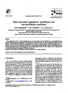
3.1. Thermodynamic State Functions of Interfacial Segregation: GI, HI, SI and VI Among the state functions of this mode, the Gibbs energy of interfacial segregation, GI, is the most important one as it completely determines interfacial concentration, XI, at temperature T for bulk atomic fraction, XIV (cf. Equation (5a)). Its importance consists in reflecting the real behavior of the system as indicated by Equation (10). Principally, GI changes not only with changing temperature but also with changing concentrations XIV and XI due to solute interaction (Figure 1). The corresponding values of HI and SI may also depend on temperature and concentration [1,5]. This means that these values can hardly provide us with any general information, e.g. about the anisotropy of grain boundary segregation, because any orientation dependence of HI and SI varies in a complex way with temperature and composition [1,5]. Figure 1. Schematic representation of the dependence of the types of GI (GI, GI° and G IE ) appearing in Equation (6) on (a) bulk concentration, and (b) temperature, both in a binary system [1].
(a)
(b) Besides GI, HI and SI, the segregation volume, VI, may be considered as another variable of equal importance. However, it seems that it has not been included in the description of interfacial segregation till now.
Entropy 2014, 16
1467
It follows from Equations (5a) and (12), that in case of a binary system M–I [13]:
dX IGB RTX GB , sat VI GB GB , sat X IGB ) dP X I (X
(15)
Integration of Equation (15) results in an expression showing that the segregation volume plays an important role in grain boundary segregation under pressure: ( P P0 )V I X IGB ( P0 ) X IGB ( P) exp GB , sat GB GB , sat GB RT X j ( P) X X j ( P0 ) X jM
(16)
jM
where P0 is the normal pressure. This relationship is principally similar to Equation (4) given by Zhang and Ren [14].
3.2. Standard Molar Thermodynamic Functions of Interfacial Segregation: G I0 , H I0 , S I0 , (c P ) 0I and VI0 The standard molar thermodynamic state functions possess a special importance in interfacial segregation as they have a very clear physical meaning. According to the definition (Equation (4)), G I0 as a combination of standard chemical potentials, is principally independent of concentration (see Figure 1a). ΔGI0 = ΔGI only if GIE 0 , i.e. if γj = γjV = 1 (Equations (5)–(7)). Certainly this represents a limitation although many systems behave nearly ideally (e.g. phosphorus in dilute Fe–P alloys [15,16]). Moreover, in an infinitesimally diluted solid solution the amount of interfacial solute enrichment is very low. Therefore it is highly probable that the solute atoms segregate at a those sites of the boundary which possess the lowest Gibbs segregation energy. Therefore, ΔGI0 characterizes the interfacial segregation of element I at a specific site of interface Φ in the ideal system. ΔHI0 and ΔSI0 are defined in analogy to ΔGI0 with corresponding physical meaning. According to Equations (3) and (8), the standard molar state functions control the relation between the activities at an interface and in the volume in the whole concentration range of a binary M–I system. Similarly to ΔGI0 and according to Equations (9a) and (9b), ΔHI° and ΔSI° are concentration independent. Analogously to ΔGI0, ΔHI0 and ΔSI0, we may define the standard molar specific heat of segregation, (c P )VI , 0 , as a combination of molar specific heats of pure substances, (c P ) j ,0 and (c P )Vj ,0 :
(c P ) 0I (c P ) I (,M0 ) (c P ) M, 0 (c P )VI (,M0 ) (c P )VM, 0 0
(17)
The value (c P ) 0I 0 results from the fact that (c P ) j ,0 are insensitive to the presence of structural defects such as dislocations as well as grain boundaries [17], i.e. although an increase of c P was reported in case of nanocrystaline materials [18]. However, the different enhancements of c P of nanocrystalline palladium and copper were ascribed to lower densities of these substances in the nanometer-sized crystalline state [18] representing transition between crystalline and glassy states. In case of a large bicrystal with specified grain boundary we may well accept the relation (c P ) j (,M0 ) (c P )Vj (,M0 ) . Then:
H I0 T
(c P ) 0I 0 P, X i
(18a)
Entropy 2014, 16
1468
and S I0 T
(c P ) 0I 0 T P, X i
(18b)
It means that ΔHI0 and ΔSI0 are independent of temperature and ΔGI0 is thus a linear function of temperature. As the standard state is defined as pure component j at temperature T and structure of M, ,0 GB , 0 ,0 V ,0 GB , 0 VIGB and VIV( M, 0 ) VMV , 0 . Consequently, VI0 VIGB VMV , 0 0 . It means that ( M ) VM ( M ) VI ( M ) VM all non-zero contributions to VI originate from the real behavior of the system (VI = VI E ). The fact that ΔVI0 = 0 has a serious consequence for other standard state functions: According to Equation (12) and (SI0/P)T = (VI0/T)P, both ΔGI0 and ΔSI0, and consequently ΔHI0 are independent of pressure. The independence of temperature and pressure is a principal property of ΔHI0 and ΔSI0 which thus change exclusively with the structure (i.e. energy) of the interface (or an interface site) and with the nature of the system. Therefore, ΔHI0 and ΔSI0 can be used for general purposes, for example, to characterize the anisotropy of interfacial segregation which is directly related to the grain boundary classification [1,5] despite their application is limited to ideal (infinitesimally diluted) systems. 3.3. Excess Thermodynamic Functions of Interfacial Segregation: G IE and VI E According to Equation (6), the excess molar Gibbs energy of segregation, G IE , represents the difference between real and ideal behavior with respect to interfacial segregation and is exactly defined by the a combination of the activity coefficients (Equation (7)). It is thus evident that G IE depends on composition and non-linearly on temperature (cf. schematic Figure 1b). However, the values of the activity coefficients are unknown and hardly measurable, particularly for interfaces. Therefore, G IE is usually approximated by various models, e.g. by the regular solid solution (Fowler) model for a binary system: X I G I 2 IM 0 (19) X where αIM is the coefficient of binary I–I interaction in M, or by various models for segregation in multicomponent systems, e.g. by the Guttmann model: E
GIE 2 IM ( X I X IV )
( X
J I ,M
IJ
J
X JV )
(20)
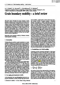
with the ternary interaction coefficients, IJ , characterizing the I–J interaction in M, where J represent other solutes in the system [10]. As only the summarizing term G IE is correlated according to the Guttmann model and the quantities H IE and S IE itself do not explicitly appear in the thermodynamic description of interfacial segregation, we will not discuss them. The effect of solute interaction (represented i.e. by IJ ) on grain boundary segregation is displayed in Figure 2. Here, the equilibrium composition is calculated for both the grain boundary of the binary M–I system in the temperature range 473–1673 K according to Equations (5) and (19) assuming a bulk concentration of XIV = 0.001 (i.e. 0.1 at.%), interstitial segregation of I at the grain boundary and the values of HIGB,0 = 30 kJ/mol and SIGB,0 = J/(mol·K) (as for P, Sb and Sn in -Fe). Figure 2
Entropy 2014, 16
1469
clearly shows the strong influence of the solute–solute interaction in the binary M–I alloy on the value of XIGB. In case of attractive interaction, IM 0, the grain boundary concentration of the segregant obviously is increased. Even in case of relatively low values of IM, e.g. IM = +10 kJ/mol, the grain boundary enrichment of I is by tens of at.% higher than without interaction (IM = 0). Repulsive interaction decreases the solute enrichment to a similar extent. This behavior is well understood because repulsive interaction does not allow putting another atom of the same kind in close surrounding of the atom segregated at the interface while attractive interaction exhibits an opposite effect [19]. The effect of ternary interactions ( IJ , Figure 2b) is much less pronounced as that of the binary interactions [20]. Figure 2. Temperature dependence of XIGB in (a) binary M–I alloy calculated according to Equations (5) and (19) using HIGB,0 = 30 kJ/mol, SIGB,0 = J/(mol K), and various values of IM [19]; and (b) ternary M–I–J alloy with additionally HJGB,0 = 10 kJ/mol, SJGB,0 = 5 J/(mol·K) and XJV = 0.03. Ibin is XIGB in the binary M–I(0.1 at.%) alloy [20].
(a)
(b)
Entropy 2014, 16
1470
Combination of Equations (12), (15) and (19) for a binary alloy with the above condition VI V I E provides us with: VI VI E
X , sat X IGB
(X
, sat
)
2
2
IM
X IGB ( X , sat X IGB )
RT
d IM dP
(21)
4. Examples of Application of Thermodynamic State Functions in Interfacial Segregation
4.1. Relationship between ΔHI0 and ΔSI0 of Grain Boundary Segregation and Volume Solid Solubility The chemical potential of the solute I at the bulk solid solubility limit, XIV,:
IV ,* IV ,0 RT ln aVI ,*
(22)
is related to the activity at the bulk solid solubility limit, aIV,*. We can express the Gibbs energy of segregation in an M–I system at the limit of solid solubility, GI*, as:
GI* I , 0 IV ,* M ,0 MV ,* GI0 RT ln aVI ,*
(23)
It follows from the basic thermodynamic relationships that: S
V ,* I
S
V ,0 I
T ln aVI ,* R T P , X Vj
(24)
Compilation of numerous literature data [21] shows that the activity of solute I at the solubility limit of numerous elements can be expressed by: aVI ,* ( X IV ,* ) v
(25)
as is apparent in Figure 3. In Equation (25), v is the exponent which is characteristic for the host element. For many binary systems, the product T lnXIV,* was found to be independent of temperature (Figure 4) [1,22]. It means that SIV,* = SIV,0 if conditions (24) and (25) are fulfilled, and: H I* H I0 RT ln aVI ,* i.e. [1,5]:
*, ( ) H I0 (, X IV ,* ) H CSS vR T ln X IV ,* (T )
(26)
(27)
*,( ) In Equation (27), H CSS is the molar enthalpy of segregation of a solute with complete volume solid solubility in solvent M, and the symbol characterizes a specific grain boundary [1,5]. As the product T lnXIV,* = const, the above mentioned condition of temperature independence of HI0 is preserved. Equation (27) represents an extension and a refinement of the expression XI/XIV = K/XIV,*, (K = 1.8–10.8) given by Hondros and Seah which relates the grain boundary enrichment ratio to the solid solubility limit [2], and the qualitative idea of Watanabe to extend this simple dependence to account for anisotropy of grain boundary segregation [23] and to construct the so called grain boundary segregation diagram. This idea was later experimentally proved [24]. The grain boundary segregation diagram for solute segregation in -iron at [100] symmetrical grain boundaries is shown in Figure 5 [1,5].
Entropy 2014, 16
1471
Figure 3. Dependence of the activity at the volume solid solubility limit, aIV,*, and corresponding atomic fraction, XIV,*, for numerous solutes in -iron correlated according to Equation (25) [1,21].
Figure 4. Temperature dependence of the product T lnXIV,* for various solutes in -iron [1,22].
Analysis of the measured data on segregation of phosphorus, silicon and carbon at individual grain boundaries in -iron show that the value of the exponent v = 0.77 [1,4,5] which is in good agreement with the value v = 0.6 obtained on basis of Equation (25) from data of Reference [21] (Figure 3). The *,( ) varies from 8 to +8 kJ/mol according to the grain boundary character (the lower value of H CSS value corresponds to highly segregated general grain boundaries while the latter one corresponds to the special grain boundaries characterized by low segregation levels: for a detailed explanation of this characterization see e.g. [1]). The above mentioned measurements of grain boundary segregation in iron [1,4,5] provided us with the values of both HI0 and SI0. As an example, the dependence of HI0 and SI0 on the misorienation
Entropy 2014, 16
1472
angle for [100] symmetrical grain boundaries is shown in Figure 6. It is obvious that the orientation dependences of HI0 and SI0 are qualitatively equivalent for all segregating elements. Figure 5. Grain boundary segregation diagram for [100] symmetrical grain boundaries in -iron [1,4,5]. Notice that the lines characterizing the dependence of HI0 on T lnXIV,* are parallel for individual grain boundaries. The value of the slope in Equation (27) is v = 0.77.
Figure 6. Anisotropy of (a) the standard enthalpy, HI0, and (b) the standard entropy, SI0, of Si, P and C segregation for [100] symmetrical grain boundaries in -iron [1,4,5].
(a)
Entropy 2014, 16
1473 Figure 6. Cont.
(b) 4.2. Compensation Effect in Grain Boundary Segregation
In principle, we can express the change of the standard molar segregation Gibbs energy of interfacial segregation, GI0, at constant temperature and pressure with a single intensive variable as [25]: G I0 dG 0 I
d. T , P ,i
(28)
Analogously, we can express HI0 and SI0 as: H I0 dH I0
S I0 d , and dS I0 j T , P ,i
d . T , P ,i
(29)
We may define a temperature TCE as:
TCE
H I0
dH I0 dS I0 S I0
d T , P ,i d T , P ,i
.
(30)
at which: dG I0 (TCE ) 0 .
(31)
It means that the change of HI0 with changing is compensated by corresponding changes of SI0 caused by a change of . Then TCE is the compensation temperature and the phenomenon is called compensation effect [1,5,26]. If we suppose that is a variable describing the structure of the grain boundary, we can read Equation (31) as providing us with the constant value of the standard Gibbs energy of a solute at any grain boundary, i.e., all grain boundaries fulfilling the above conditions exhibit the same level of grain boundary segregation. If represents the nature of the solute, all grain
Entropy 2014, 16
1474
boundaries will exhibit the same value of the grain boundary enrichment ratio, XI/XIV. The former case is documented for example on the basis of experimental data for phosphorus segregation at individual grain boundaries of -iron in Figure 7. Let us note that condition (31) does not identify a phase transformation characterized by minimum of the Gibbs energy: phase transformation is a subcategory of the compensation effect. At TCE no transformation of the boundaries occurs but they coexist besides each other, despite the temperature changes in the vicinity of TCE [25,27]. Integration of Equation (30) results in [1,5]: S I0 ( ) S 0,CE
H I0 ( ) . TCE
(32)
Figure 7. Temperature dependence of the standard Gibbs energy of phosphorus segregation, GP0, in -iron at various [100] symmetrical grain boundaries in [1,5].
The plot of the relation between HI0 and SI0 for solute segregation in -iron is shown in Figure 8. We can distinguish two branches of this dependence: they differ in the type of segregation site: the upper one corresponds to interstitial segregation (S0,CE = 56 J/(mol·K)) while the lower one to substitutional segregation (S0,CE = 5 J/(mol·K)) [1,4,5]. Individual full symbols of the same type correspond to the segregation of a solute at individual grain boundaries in -iron, empty symbols are data found in literature (for the sources of the data, see [1,5]). Let us note that various solutes segregating at the same type of the site also fit with a single dependence (i.e. with either upper or lower branch in Figure 8). The slope of both dependences corresponds to TCE = 930 K which suggests that the compensation temperature is characteristic for the matrix [1,5,28]. Splitting of the compensation effect into two branches confirms the fact that the compensation effect is only fulfilled if a single mechanism of the phenomenon is active. Therefore, it can be applied to otherwise independent standard quantities HI0 and SI0 albeit not to HI and SI which additionally change with temperature and composition.
Entropy 2014, 16
1475
Figure 8. Compensation effect in solute segregation at [100] symmetrical grain boundaries in -iron [1,4,5]. Upper branch corresponds to interstitial segregation, lower branches to substitutional one.
Let us only briefly mention that Equations (27) and (32) with the above mentioned values of *,( ) H CSS and S0,CE can be used to predict the values of HI0 and SI0 of any element at any grain boundary in -iron [1,4,5]. It is likely that such prediction may be done for other metallic solvents. We can also express the dependence of SI0 on the volume solid solubility. Combination of Equations (27) and (32) provides us with: S (, site, X 0 I
V ,* I
*, ( ) 0,CE vR H CSS ) S (, site) T ln X IV ,* (T ) TCE TCE
(33)
where the notation site refers to the type of segregation, i.e., either interstitial or substitutional. Using the mentioned data, dependence (33) is shown in Figure 9. It is clearly seen that the majority of the experimental data corresponding to both individual grain boundaries (solid symbols) and to grain boundaries in polycrystals found in the literature (empty symbols) fit fairly well to the theoretical lines of individual branches (the upper line of each branch corresponds to special boundaries while the lower one to general boundaries). The compensation effect was observed not only in case of grain boundary and surface segregation but also for other interfacial properties, such as grain boundary migration and diffusion [5,26,27], and is present in many phenomena of physics, chemistry and biology [25].
4.3. Segregation Volume and Pressure Dependence of Grain Boundary Segregation During time-dependent experimental studies of non-equilibrium segregation under constant stress, in the beginning a steep change of the grain boundary concentration is observed, followed by the return from an extreme value to a value almost corresponding to that measured without pressure or strain; see e.g. Figure 10 according to Reference [29]).
Entropy 2014, 16
1476
According to Equation (14) (where we use for simplicity X,sat = XGB,sat = 1, which is often applied in correlation of data on grain boundary segregation [1]), VI E can be obtained from experimental data [29] on pressure/stress dependence of grain boundary segregation of solutes. According to our method [30] the peak-to-peak heights in original Auger spectra were transformed into concentrations supposing simplification of the alloy to a binary Fe–P system. This procedure provides us with the values of XPGB = 0.303 representing the state under normal pressure and XPGB = 0.308 for the state in the stressed sample after equilibration (Figure 10). According to Equation (14) we obtain VPE 5.1 × 10⁶ m3/mol [13]. Similar value VSE 5.5 × 10⁶ m3/mol for sulphur was determined from the data of Misra [31] who studied grain boundary segregation of sulphur in a low-alloy steel (doped by 0.01 wt.% S) under plastic stress conditions at 883 K by 343 MPa. However, no changes of XPGB were observed after prolonged annealing of a phosphorus-doped 2.25Cr1Mo steel at 793 K under various loads [32] suggesting VPE = 0 and thus, ideal behavior of this system. Figure 9. Dependence of standard entropy of grain boundary segregation in -iron on the volume solid solubility term, (T lnXIV,*)/TCE. Solid symbols refer to segregation at individual grain boundaries [4,5], empty symbols are literature data corresponding to measurements on polycrystals [1]. The dashed lines were calculated according to Equation (33).
The value of V I E can also be estimated in other ways. First, VFebulk 7.1 × 10⁶ m3/mol if pure Fe is considered instead of the 2.6NiCrMoV steel [33]. As the average boundary density is of about 50% of the bulk density [33], VFeGB 1.42 × 10⁵ m3/mol. Based on the density of FeS (4.82 g/cm3 [34]), VSGB 1.76 × 10⁵ m3/mol if GB is regarded as a Fe-48 at.%S since the atomic fraction of S in 2.6NiCrMoV is 48 at.% after stress-aging for 20 h [35]. Then VSbulk 0.0002 × VFebulk 1.4 × 10⁹ m3/mol, and VSE = 1.0 × 10⁵ m3/mol. On the other hand, the values of VSE = 8.1 × 10⁶ m3/mol, 6 3 6 3 V PE = 3.0 × 10 m /mol and VSeE = 3.0 × 10 m /mol were calculated using the density functional theory technique for segregation of S, P and Se, respectively, at {012} grain boundary in Ni [36].
Entropy 2014, 16
1477
Figure 10. Time dependence of grain boundary segregation of phosphorus in a 0.05 wt% P-doped low alloy steel at 773 K under tensile (▲) or compressive (●) stress of 30 MPa (according to Reference [29]).
The value of VI E of the order of 106105 m3/mol may seem to be low. It suggests that the pressure dependence of GI and consequently of XIGB is rather low: Even the value of VI E 1 × 10⁵ m3/mol under pressure/stress of 100 MPa causes a decrease of GI by 1 kJ/mol which represents a change of XIGB in the order of several percent. This also explains why the equilibrium segregation under pressure only slightly differs from that under normal pressure [29] (see Figure 10). Let us now consider the effect of VI E on XIGB in more detail. Supposing the values HI0 =
30 kJ/mol and SI0 = 25 J/(mol·K) (these values may represent e.g. phosphorus segregation in bcc iron [1]) and XIV = 0.0001, the grain boundary concentration of the solute under normal pressure at temperature of 800 K is XIGB(P = 0) = 0.1554 (i.e. 15.54 at.%). The pressure dependence of the calculated XIGB is plotted in Figure 11 for the values of VI E ranging from 8 × 10⁶ m3/mol to 0. It is obvious from Figure 11 that XIGB starts to change when the pressure is higher than 10 MPa: under these higher pressures the increase of XIGB becomes quite steep. We may conclude that although the effect of elastic deformation on grain boundary segregation is small the grain boundary segregation significantly changes with increasing pressure. At high hydrostatic pressures (P 10 GPa) this effect is rather large: In this case, the equilibrium grain boundary concentration should reach the values up to 100 at.% (cf. Figure 11) [13]. However, during such treatment many other processes occur in the material, e.g. dynamic recrystallization, which will influence the final segregation level; in the present modeling these effects were not taken into account. Similarly to the basic thermodynamic state variables of segregation (HI0 and SI0; cf. Figure 6) we may expect that VI E will be anisotropic. Supposing HI0 = 30 kJ/mol, SI0 = 25 J/(mol·K) and VI E = 5 106 m3/mol, and HI0 = 10 kJ/mol, SI0 = 40 J/(mol·K) with VI E = 2 106 m3/mol describe segregation of I at general and special grain boundary, respectively, the pressure dependence of XIGB for both types of the grain boundaries at 800 K is shown in Figure 12 for XIV = 0.0001. As expected, the segregation level is lower at the special grain boundary compared to the general one. The concentration change at the special grain boundary requires higher pressure.
Entropy 2014, 16
1478
However, its increase may seem to be surprisingly steeper than in case of the general grain boundary. In both cases a complete saturation of the grain boundary is reached under ultimate pressures. Figure 11. Pressure dependence of XIGB in a model M–I(0.01 at.%) alloy at 800 K for various values of VI E as indicated at the curves (in 106 m3/mol) [13].
Figure 12. Pressure dependence of XIGB at special and general grain boundaries in a model M–I(0.01 at.%) alloy at 800 K. The values HI° = 30 kJ/mol, SI° = 25 J/(mol·K) and 6 3 V I E = 5 10 m /mol were used for general grain boundary, and HI° = 10 kJ/mol, SI° = 40 J/(mol·K) and VI E = 2 106 m3/mol for special grain boundary [13].
The segregation volume VI E depends on various intensive variables. We will document it for example of XIV and T. Differentiation of Equation (15) provides us with:
Entropy 2014, 16
1479
VI E V X I
RTX GB , sat GB GB , sat X IGB ) T , P X I ( X X GB , sat 2 X GB X GB 2 X IGB X IGB GB GB , sat I GB I X I ) P T , X V X IV T , P PX IV X I ( X I
T
(34)
The first term at the right-hand side (in front of the brackets) is positive as well as the first (left) one in the brackets (supposing that less than half of the saturation limit is segregated) as XIGB increases with increasing both pressure and XIV. The sign of VI E X IV (i.e. slope of the concentration dependence of the segregation volume) will depend on the value of the term 2 X IGB PX IV . Intuitively, we may expect the decrease of VI E (i.e. increase of its absolute value) with increasing XIV (and thus with increasing XIGB). For this case, 2 X IGB PX IV should be positive and prevail over the first term in the brackets on the right hand side of Equation (34). In analogy to Equation (34), the dependence of V I E on temperature is characterized by: VI E T
RTX GB ,sat GB GB ,sat X IGB ) X I (X P , X VI 1 X GB ,sat 2 X GB X GB GB GB ,sat I GB I X I ) T P , X V T X I ( X I
X IGB 2 X IGB P T , X VI PT X VI
(35)
We may expect that (negative) value of VI E increases with increasing temperature and reaches the value VI E 0 at high temperatures (e.g. close to the melting point). To bring this expectation in accordance with Equation (35), the term in the complex brackets should be positive. As X IGB P is positive and X IGB T negative (segregation decreases with increasing temperature), the term in the edge brackets on the right-hand side of Equation (35) is negative. Therefore, 2 X IGB PT on the right-hand side of Equation (35) must be negative and of higher absolute value than the other term in the complex brackets. Then VI E / T P , X VI > 0. Based on Equation (21) we may demonstrate the effect of pressure on the Fowler interaction coefficient, IM (cf. Equation (19)), as:
IM
d IM RT dP
1 X IGB ( X GB , sat X IGB ) ( X GB , sat ) 2 2 VI E . GB , sat GB X XI
(36)
Supposing XGB,sat = 1 and XIGB >> XIV, we obtain: d IM 1 VI E IM (1 X IGB ) . dP 2 X IGB RT
(37)
The concentration dependences of the value of dIM/dP for various values of IM and VI E are shown in Figures 13 and 14. It is obvious that the value of the fraction on the right-hand side of Equations (36) and (37) is of the order of units in case of high grain boundary concentrations. It means that the value of dIM/dP is of the same order as VI E , i.e. at the level of 106 m3/mol. This suggests that a change of IM by 1 kJ/mol results in an apparent change of X IGB when pressure or stress reaches values of the order of hundreds of MPa. The change of IM with pressure is more
Entropy 2014, 16
1480
pronounced for low grain boundary concentrations, however, the interaction in case of the dilute alloys can be neglected (cf. Equation (19)). It means that, usually, the pressure change of the interaction coefficient can be neglected. Figure 13. Concentration dependence of dIM/dP for various values of IM (in units of RT) in a binary M–I alloy for the value of VI E = 5 × 10⁶ m3/mol.
Figure 14. Concentration dependence of dIM/dP for various values of VI E in a binary
M–I alloy (in 106 m3/mol) for IM = 2RT.
Entropy 2014, 16
1481
5. Conclusions
Application of basic thermodynamics to a field of material science with important practical consequences—interfacial segregation—is presented in detail. Based on the Langmuir–McLean segregation isotherm, individual modes of thermodynamic intensive variables—which are used to describe this phenomenon—are discussed from the point of view of their physical meaning together with their potential for application. To the best of our knowledge, the segregation volume is fully defined and discussed for the first time here. It is shown that the standard molar segregation volume is zero at any temperature according to the definition of the standard states while the partial molar excess segregation volume reaches non-zero values in real systems. It is concluded that the grain boundary segregation is not affected by pressure in ideal systems whereas the real systems exhibit apparent pressure dependence. The dependences of the standard molar enthalpy of segregation on the bulk solid solubility and the enthalpy–entropy compensation effect are displayed to enable formulation of a relationship between the standard molar entropy of grain boundary segregation and the volume bulk solid solubility. In addition, a fundamental relationship is derived between the segregation excess volume and pressure changes of the grain boundary concentration of the segregant, and various important consequences of the segregation volume are established. Acknowledgments
This work was supported by the Czech Science Foundation (Projects No. GAP108/12/0144 (PL) and GAP108/12/0311 (MŠ)), by the Project CEITEC—Central European Institute of Technology (CZ.1.05/1.1.00/02.0068) from the European Regional Development Fund (MŠ), by the Academy of Sciences of the Czech Republic (Institutional Project RVO:68081723 (MŠ)), by the National Natural Science Foundation of China (Project No. 51001011 (LZ)) and by the Fundamental Research Funds for the Central Universities (Project No. FRF-TP-12-042A (LZ)). Author Contributions
This paper was prepared in close cooperation of all four co-authors: Pavel Lejček and Siegfried Hofmann provided the main contribution to the thermodynamics of grain boundary segregation and its anisotropy including the enthalpy–entropy compensation effect. Pavel Lejček and Lei Zheng elaborated the idea of the segregation volume which was later completed by Mojmír Šob for the theoretically calculated data. Pavel Lejček wrote the draft of the article which was critically revised by all other co-authors and finalized in the agreement of all co-authors. All co-authors also approved the final version. Conflicts of Interest
The authors declare no conflict of interest. References
1.
Lejček, P. Grain Boundary Segregation in Metals; Springer: Heidelberg, Germany, 2010.
Entropy 2014, 16 2. 3. 4. 5. 6. 7. 8. 9. 10. 11. 12. 13. 14. 15. 16.
17. 18. 19. 20. 21. 22.
23. 24.
1482
Hondros, E.D.; Seah, M.P. Segregation to interfaces. Int. Met. Rev. 1977, 22, 262–299. Johnson, W.C.; Blakely, J.M., Eds.; Interfacial Segregation; ASM: Metals Park, OH, USA, 1979. Lejček, P.; Hofmann, S. Thermodynamics and structural aspects of grain boundary segregation. Crit. Rev. Solid State Mater. Sci. 1995, 20, 1–85. Lejček, P.; Hofmann, S. Thermodynamics of grain boundary segregation and applications to anisotropy, compensation effect and prediction. Crit. Rev. Solid State Mater. Sci. 2008, 33, 133–163. DuPlessis, J. Surface segregation. Solid State Phenom. 1990, 11, 1–125. Wynblatt, P.; Chatain, D. Anisotropy of segregation at grain boundaries and surfaces. Metall. Mater. Trans. 2006, 37, 2595–2620. Polak, M.; Rubinovich, L. The interplay of surface segregation and atomic order in alloys. Surf. Sci. Rep. 2000, 38, 127–194. Lewis, G.N.; Randall, M. Thermodynamics; McGraw–Hill: New York, NY, USA, 1923. Guttmann, M.; McLean, D. Grain boundary segregation in multicomponent systems. In Interfacial Segregation; Johnson W.C., Blakely, J.M., Eds.; ASM: Metals Park, OH, USA, 1979; pp. 261–348. Sutton, A.P.; Balluffi, R.W. Interfaces in Crystalline Solids; Clarendon: Oxford, UK, 1995. Lojkowski, W. Evidence for pressure effect on impurity segregation in grain boundaries and interstitial grain boundary diffusion mechanism. Defect Diffus. Forum 1996, 129–130, 269–278. Lejček, P.; Zheng, L.; Meng. Y. Excess volume in grain boundary segregation. J. Surf. Anal. 2014, 20, 198–201. Zhang, T.-Y.; Ren, H. Solute concentrations and strains in nanograined materials. Acta Mater. 2013, 61, 477–493. Erhart, H.; Grabke, H.J. Equilibrium segregation of phosphorus at grain boundaries of Fe–P, Fe–C, Fe–Cr–P, and Fe–Cr–C–P alloys. Metal Sci. 1981, 15, 401–408. Janovec, J.; Grman, D.; Perháčová, J.; Lejček, P.; Patscheider, J.; Ševc, P. Thermodynamics of phosphorus grain boundary segregation in polycrystalline low-alloy steels. Surf. Interf. Anal. 2000, 30, 354358. Cottrell, A.H. Theoretical Physical Metallurgy; Edward Arnold Publ.: London, UK, 1959. Rupp, J.; Birringer, R. Enhanced specific-heat-capacity (cp) measurements (150–300 K) of nanometer-sized crystalline materials. Phys. Rev. B 1987, 36, 7888–7890. Lejček, P. Effect of solute interaction on interfacial segregation and grain boundary embrittlement in binary alloys. J. Mater. Sci. 2013, 48, 2574–2580. Lejček, P. Effect of ternary solute interaction on interfacial segregation and grain boundary embrittlement. J. Mater. Sci. 2013, 48, 4965–4972. Hultgren, R.; Desai, P.; Hawkins, D.; Gleiser, M.; Kelley, K., Eds. Selected Values of the Thermodynamic Properties of Binary Alloys; ASM: Metals Park, OH, USA, 1973. Kubaschewski, O. Iron—Binary Phase Diagrams; Springer: Berlin, Germany, 1987; Massalski, T.B. Binary Alloy Phase Diagrams; ASM: Metals Park, OH, USA, 1987; Predel, B. Phase Equilibria of Binary Alloys; Springer: Berlin, Germany, 2003. Watanabe, T.; Kitamura, S.; Karashima, S. Grain boundary hardening and segregation in -iron–tin alloy. Acta Metal. 1980, 28, 455–463. Hofmann, S.; Lejček, P. Correlation between segregation enthalpy, solid solubility and interplanar spacing of = 5 tilt grain boundaries in -iron. Scripta Metall. Mater. 1991, 25, 2259–2262.
Entropy 2014, 16
1483
25. Lejček, P. Enthalpy–entropy compensation effect in grain boundary phenomena. Z. Metallkd. Int. J. Mater. Res. Adv. Tech. 2005, 96, 1129–1133. 26. Gottstein, G.; Shvindlerman, L.S. Grain Boundary Migration in Metals; CRC Press: Boca Raton, FL, USA, 1999. 27. Lejček, P. Is the compensation effect a phase transition? Solid State Phenom. 2008, 138, 339–346. 28. Lejček, P.; Jäger, A.; Gärtnerová, V. Reversed anisotropy of grain boundary properties and its effect on grain boundary engineering. Acta Mater. 2010, 58, 1930–1937. 29. Shinoda, T.; Nakamura, T. A model for the applied stress effects on the intergranular phosphorus segregation in ferrous materials. Acta Metall. 1981, 29, 1637–1644. 30. Lejček, P. On the determination of surface composition in Auger electron spectroscopy. Surf. Sci. 1988, 202, 493–508. 31. Misra, R.D.K. Issues concerning the effect of applied tensile stress on intergranular segregation in a low alloy steel. Acta Mater. 1996, 44, 885–890. 32. Song, S.-H.; Wu, J.; Weng, L.-Q.; Liu, S.-J. Phosphorus grain boundary segregation under different applied tensile stress levels in a Cr–Mo low alloy steel. Mater. Lett. 2010, 64, 849–851. 33. Jorra, E.; Franz, H.; Peisl, J.; Petry, W.; Wallner, G.; Birringer, R.; Gleiter, H.; Haubold, T. Small-angle neutron scattering from nanocrystalline Pd. Phil. Mag. B 1989, 60, 159–168. 34. Speight, J.G. Lange’s Handbook of Chemistry; McGraw-Hill: New York, USA, 2005; Table 4-1. 35. Xu, T.D. Grain-boundary anelastic relaxation and non-equilibrium dilution induced by compressive stress and its kinetic simulation. Phil. Mag. 2007, 87, 1581–1599. 36. Všianská, M.; Šob, M. Central European Institute of Technology, CEITEC MU, Masaryk University, Brno, Czech Republic. Unpublished data, 2013. © 2014 by the authors; licensee MDPI, Basel, Switzerland. This article is an open access article distributed under the terms and conditions of the Creative Commons Attribution license (http://creativecommons.org/licenses/by/3.0/).