INTERSPEECH 2017 August 20–24, 2017, Stockholm, Sweden
Approaches for Neural-Network Language Model Adaptation Min Ma1∗, Michael Nirschl2 , Fadi Biadsy2 , Shankar Kumar2 1
Graduate Center, The City University of New York, NY, USA 2 Google Inc, New York, NY, USA
[email protected], {mnirschl, biadsy, shankarkumar}@google.com
Abstract
queries). Since written and spoken language may differ in terms of syntactic structure, word choice and morphology [8], a language model of an ASR system is likely to benefit from training on spoken, in-domain training data, to alleviate the mismatch between training and testing distributions. Since there are limited quantities of manually transcribed data available to train the LM, one might train it on unsupervised transcriptions generated by ASR systems in the domain of interest. However, by doing so, we would potentially reinforce the errors made by the ASR system. The solution we propose in this paper to address this mismatch is to pre-train an LM on large written textual corpora, and then adapt it on the given manually transcribed speech data of the domain of interest. This will enable the model to learn co-occurrence patterns from text with broad coverage of the language, likely leading to good generalization, while focusing on features specific to the spoken domain. In this paper, we first train a background model on a large corpus of primarily typed text with a small fraction of unsupervised spoken hypotheses, then update part of its parameters on a relatively small set of speech transcripts using our three adaptation strategies. Compared to feed-forward Deep Neural Network (DNN) LMs, the adaptation of Recurrent Neural Network (RNN) LMs is an active research area [9]. In this paper, both DNN and recurrent neural network (LSTM) architectures were explored. We investigate a number of training techniques for enhancing model performance of large-scale NNLMs, and illustrate how to accelerate pre-training as well as adaptation.
Language Models (LMs) for Automatic Speech Recognition (ASR) are typically trained on large text corpora from news articles, books and web documents. These types of corpora, however, are unlikely to match the test distribution of ASR systems, which expect spoken utterances. Therefore, the LM is typically adapted to a smaller held-out in-domain dataset that is drawn from the test distribution. We propose three LM adaptation approaches for Deep NN and Long Short-Term Memory (LSTM): (1) Adapting the softmax layer in the Neural Network (NN); (2) Adding a non-linear adaptation layer before the softmax layer that is trained only in the adaptation phase; (3) Training the extra non-linear adaptation layer in pre-training and adaptation phases. Aiming to improve upon a hierarchical Maximum Entropy (MaxEnt) second-pass LM baseline, which factors the model into word-cluster and word models, we build an NN LM that predicts only word clusters. Adapting the LSTM LM by training the adaptation layer in both training and adaptation phases (Approach 3), we reduce the cluster perplexity by 30% on a held-out dataset compared to an unadapted LSTM LM. Initial experiments using a state-of-the-art ASR system show a 2.3% relative reduction in WER on top of an adapted MaxEnt LM. Index Terms: neural network based language models, language model adaptation, automatic speech recognition
1. Introduction Language models (LMs) play an important role in Automatic Speech Recognition (ASR). In a two-pass ASR system, two language models are typically used. The first is a heavily pruned n-gram model which is used to build the decoder graph. Another larger or more complex LM is employed to rescore hypotheses generated in the initial pass. In this paper, we focus on improving the second-pass LM. Recently, Neural Network Language Models (NNLMs) have become a popular choice for large vocabulary continuous speech recognition (LVCSR) [1, 2, 3, 4, 5, 6]. A LM assigns a probability to a word w given the history of preceding words, h. Unlike an n-gram LM, a neural network LM maps the word and the history to a continuous vector space using an embedding matrix and then computes the probability P (w|h) making use of a similarity function in this space. This continuous representation has been shown to result in better generalization relative to n-gram LMs [2]. Furthermore, it can be exploited when adapting to a target domain with limited supervision [7]. In this paper, we explore a variety of NNLM adaptation strategies for rescoring hypotheses generated by an ASR system. LMs used in ASR systems are typically trained on written text (e.g. web documents, news articles, books or typed ∗This
2. Previous Work Mikolov and Zweig [10] extended the basic RNN LM with an additional contextual layer which is connected to both the hidden layer and the output layer. By providing topic vectors associated with each word as inputs to the contextual layer, the authors obtained a 18% relative reduction in Word Error Rate (WER) on the Wall Street Journal ASR task. Chen et al. [11] performed multi-genre RNN LM adaptation by incorporating various topic representations as additional input features, which outperformed the RNN LMs that were fine-tuned on genre specific data. Experiments showed an 8% relative gain in perplexity and a small WER reduction compared to an unadapted RNN LMs on broadcast news. Deena et al. [9] extended this work by incorporating a linear adaptation layer between the hidden layer and output layer, and only fine-tuning its weight matrix when adapting. Combining the model-based adaptation with Chen et al’s [11] feature based adaptation, Deena et al. reported a 10% relative reduction in perplexity and a 2% relative reduction in WER, also on broadcast news. Techniques from acoustic model adaptation such as learning hidden unit contribution [12], linear input network [13] and linear hidden network [14], have been borrowed for adaptation
work was done while Min Ma was an intern at Google.
Copyright © 2017 ISCA
259
http://dx.doi.org/10.21437/Interspeech.2017-1310
of LMs. For example, Gangireddy et al. [15] obtained moderate WER reductions by re-weighting the hidden units based on their contributions in modeling the word distributions for multigenre broadcast news. Park et al. [7] inserted a linear adaptation layer between the embedding and the first hidden layer in an DNN LM. During adaptation, only the adaptation layer was updated using 1-best hypotheses for supervision. When combined with a 4-gram LM, the adapted DNN LM decreased the perplexity by up to 25.4% relative, and yielded a small WER reduction in an Arabic speech recognition system where it was used as a second-pass LM.
i-th output = P (ct = cm |context)
i-th output = P (wt = wn |context) Word Softmax
Cluster Softmax
(training only) recurrent connection
LSTM Layer
Embeddings shared parameters across clusters
3. Data wi
We conduct all experiments on an Italian speech recognition task. We use a large corpus of typed texts consisting of aggregated and anonymized typed queries from Google Search, Google Maps and crawled web documents, which make up a total of more than 29 billion sentences (about 114 billion word tokens). We add a small amount (< 0.5%) of unsupervised spoken hypotheses and use the entire corpus as the training set of the background LM. The spoken texts consist of speech transcripts collected from a mixture of voice queries and dictation, and are split into two independent sets by time period: adaptation set (i.e. the training data in adaptation phase), which includes approximately 2.6 million sentences (about 16 million word tokens); development set, which is composed of about 1.2 × 10⁵ sentences (about 6 × 10⁵ word tokens). We evaluate perplexities on the development set and report the WER results for the top performing adapted LMs using a state-ofthe-art ASR system on a dedicated ASR test set. All the aggregated voice queries (which contain short and long queries) 1 are anonymized. The modelled vocabulary contains 1 million words, which were grouped into 1003 clusters using an adaptation of the Brown algorithm [16, 17].
n+1
ci
n+1
wi
n+2
shared parameters across words
ci
n+2
wi
1
ci
1
Figure 1: Architecture of LSTM LM. and fed to the hidden layers which consist of two layers for DNN and one layer for LSTM, followed by two independent softmax layers (i.e. word and cluster softmax layers). LSTM LM is shown in Figure 1, DNN LM is similar except for the non-recurrent hidden layer. Although the NNLM is trained for the cluster prediction task, we have seen that adding the word level softmax layer for training improves the accuracy on cluster prediction. We employ a sampled softmax loss with 8192 negative samples to accelerate the training of the word softmax layer [20]. We borrow the formulations for DNN LM from [3] and for LSTM LM from [21]. Our DNN LM is a 5-gram, 2layer model with 8192 nodes in each layer. Our LSTM LM consists of one LSTM layer with 8192 nodes and a 1024 dimensional internal projection layer. We implement LSTM LM using an augmented setting proposed in [21]. A peephole connection from its internal cells to the gates in the same cell is used. We couple the input gate to 1.0 minus forget-gate to restrict the internal state of the LSTM cell to the unit interval. An internal projection is applied both in the recurrent loop and before passing the features to softmax layers. The projection strategy helps minimize computational cost while maintains the memory capacity of the model.
4. Language Models 4.1. Maximum Entropy based Language Model The baseline is a LM trained under the maximum entropy criterion. Since our word vocabulary is very large, estimating a probability distribution over the entire vocabulary becomes expensive. To reduce computational cost, we employ a hierarchical approach proposed in [18] that first predicts a cluster of words and then predicts a word from the chosen cluster. We focus on the task of improving cluster prediction because the smaller cluster vocabulary makes training easier and allows for adaptation while minimizing the risk of overfitting on the smaller adaptation dataset. The baseline MaxEnt LM consists of 5 billion parameters, adapted on the same adaptation set, the details of the baseline LM and the adaptation methodology can be found in Biadsy et al. [19].
4.3. Model Training We train the models for cluster prediction, whose smaller softmax vocabulary makes training more efficient and less prone to overfitting on our adaptation dataset. In the context of ASR, we interpolate the NNLM and MaxEnt cluster costs and use the MaxEnt word cost to assign the final score of second-pass, i.e. logP (W |h)2nd−pass = logPM E (W |C, h)+ (1) (1 − wN N ) × logPM E (C|h) + wN N × logPN N (C|h) where wN N is the weight of the NNLM. The log probability assigned by the second-pass LM logP (W |h)2nd−pass is linearly interpolated with the log probability from the first-pass LM using an interpolation weight of 0.5. We use regular back-propagation to train the DNN LM. We train the LSTM LM with truncated backpropagation through time [22] with an unrolling of 20 time steps. Training loss is defined as the cross entropy between predicted cluster labels and reference cluster labels. Mini-batch stochastic gradient descent (SGD) [23] is used with an Adagrad [24] optimizer and a batch size of 128 sequences. We use a learning rate of 0.01 for the DNN LM, and 0.2 for the LSTM LM. We found it crucial to use gradient clipping on the LSTM gradients (clipping L2-norm ≤ 1.0). In order to prevent models from overfitting, we employ
4.2. Neural Network based Language Models In this paper, the input to the NNLM consists of both words and the corresponding clusters, which are encoded by separate embedding layers. Each word (cluster) is first represented by a 1-of-k encoding (all the out-of-vocabulary words are mapped to an token) and then mapped to the embedding space (2048 dimension for words, 40 for clusters). The dense representations of the word and cluster contexts are concatenated 1 The average number of words per sentence/utterance is 3.9 for the training set, 6 for the adaptation set and 5 for the development set.
260
i-th output = P (ct = cm |context)
dropout [25] regularization (with dropout probability 0.2) to the input and output of the hidden layers for all NNLMs. We also utilize zoneout [26] for regularizing the DNN adaptation layer as explained in Section 5.
(training only)
Embeddings shared parameters across clusters
wi
n+1
ci
n+1
wi
shared parameters across words
n+2
ci
n+2
wi
1
ci
1
Figure 2: Add adaptation layer in LSTM LM. work to use already learnt features in lower layers better, we add the adaptation layer between the hidden layer and softmax layers. This approach is conceptually similar to the linear hidden layer for acoustic model adaptation [14], but we specify the adaptation layer as a single-layer neural network adaptation layer (NNadapt) with 1024 nodes and ReLU activation. We use a non-linearity to learn a function that is potentially more complex than the linear transformation in the softmax layer. We note that the NNadapt layer does not exist in pre-training phase in Scheme II. In fine-tuning phase, we update cluster softmax and NNadapt layers and keep the parameters of other layers fixed. As shown in Table 2, Scheme II helps the DNN LM reduce cluster perplexity to 34, slightly better than Scheme I. This indicates the NNadapt layer learns some information that is specific to the speech domain in the adaptation phase. Adapted performance of LSTM LMs stays the same as Scheme I.
We fine-tune only the cluster softmax layer. This is motivated by the observation that transfer learning becomes easier and more effective with high-level abstract features [27]. We do not fine-tune the entire model as the amount of adaptation data is considerably smaller than the number of parameters ( ≈ 109 for word embeddings). Training the DNN background LM is about 3 times slower than the LSTM background LM but converges to the same test cluster perplexity of 46 (Table 1). All perplexity numbers refer to the cluster prediction task. The DNN LM using Scheme I successfully reduces cluster perplexity on development data by 23.9% relative while the LSTM LM reduces cluster perplexity by 26.1% relative. Since the word softmax was helpful while training the background model, we add a word softmax (wordSF) layer to the adaptation procedure (denoted as “+ wordSF”). As shown in Table 1, including word softmax does not make a difference for DNN LM, but slightly hurts the performance of LSTM LM (only 23.9% for + wordSF). This indicates that the benefits from word softmax do not extend to the adapted model. More experiments are conducted to ascertain the necessity of freezing the hidden layers. We exploit various freezing settings and find: 1) adapting hidden layers of DNN LM only reduced cluster perplexity by 6.5% relative; adapting hidden layers of LSTM LM overfits; 2) Adapting all layers makes both DNN and LSTM LMs overfit.
Table 2: Cluster perplexity on development set of pre-trained model (“pre”), adapted model (“post”) and relative changes. Model and Adaptation Strategy DNN LM using Scheme II + wordSF LSTM LM using Scheme II + wordSF
pre 46 46
post 34 34 34 34
∆ PPL -26.1% -26.1% -26.1% -26.1%
5.3. Scheme III - Add DNN layer in Pre-training and Adaptation In Scheme II, the NNadapt layer is randomly initialized and fine-tuned on limited amounts of adaptation data. To further improve its performance, we add NNadapt in both the pre-training and fine-tuning phases (shown in Figure 2), attempting to provide a better initialization to the adaptation layer. Since the adaptation layer is a feedforward layer, we scale down its gradients by a factor of 10. We found in our experiments that it is best to apply dropout regularization on the input and output of DNN/LSTM layers and zoneout regularization for the NNadapt layer. Standard training schemes based on random initialization tend to place the parameters in regions of the parameter space that generalize poorly [28]. Hence if we initialize the weight matrix of NNadapt layer with an identity matrix (closer to a reasonable operating point), training will be substantially accelerated (by a factor of 3X). The LSTMNNadapt architecture is the strongest background model as the pre-trained cluster perplexity reduces to 43 (better than back-
Table 1: Cluster perplexity on development set of pre-trained model (“pre”), adapted model (“post”) and relative changes.
46
recurrent connection
LSTM Layer
5.1. Scheme I - Fine-tune Softmax Layer
post 29 35 35 43 34 35
ReLu
Adaptation Layer
We adopt a “pre-train and fine-tune” methodology in all our adaptation schemes. In the first phase, we train a background LM on the entire training set and test it on the development set. We use the converged model to initialize the adaptation stage. In the second phase, fine-tuning (a.k.a. adaptation), we freeze some layers of the model, i.e. we do not update the weight matrices of the frozen layers when back-propagating. Only the weights of unfrozen layers get fine-tuned (shown as red bold arrows in Figure 1 and 2). All the adaptation strategies investigated only take up to an additional 13% time to achieve optimal performance.
pre 40 46
Word Softmax
Cluster Softmax
5. Adaptation Approaches
Model and Adaptation Strategy MaxEnt Baseline LM DNN LM using Scheme I + wordSF + wordSF, + DNN LSTM LM using Scheme I + wordSF
i-th output = P (wt = wn |context)
∆ PPL -27.5% -23.9% -23.9% -6.5% -26.1% -23.9%
5.2. Scheme II - Add Adaptation Layer when Fine-tuning We add an adaptation layer to the NNLMs with a limited amount of parameters to avoid overfitting. To allow the net-
261
ground LMs in Scheme I and II by 6.5% relative). When finetuning, we update cluster softmax and NNadapt layers in the LSTM-NNadapt model (Scheme III). Variants which include wordSF in fine-tuning are applicable to both NNLM architectures. Since the DNN-NNadapt architecture is equivalent to a 3-layer DNN LM, and no significant gain was seen in the experiments, we do not discuss it further. Experimental results of LSTM LM are shown in Table 3. We found that fine-tuning only the cluster softmax achieved the best adapted cluster perplexity reduction of 30.2% relative. Finetuning both cluster and word softmax yielded the second best adapted performance. However, once we included the LSTM layer in fine-tuning (“+ LSTM”), the model showed overfitting.
Table 4: WER results and relative changes of ASR system based on different non-adapted or adapted language models. Language Model non-adapted MaxEnt adapted MaxEnt baseline non-adapted DNN (I) non-adapted DNN (I) adapted DNN (I) adapted DNN (I) non-adapted LSTM (I) non-adapted LSTM (I) adapted LSTM (I) adapted LSTM (I) non-adapted LSTM (III) non-adapted LSTM (III) adapted LSTM (III) +wordSF adapted LSTM (III) +wordSF
Table 3: Cluster perplexity on development set of pre-trained model (“pre”), adapted model (“post”) and relative changes. Model and Adaptation Strategy LSTM LM using Scheme III + wordSF + wordSF, + LSTM
pre 43
post 30 31 198
∆ PPL -30.2% -27.9% +360.5%
wN N 0.0 0.0 0.5 1.0 0.5 1.0 0.5 1.0 0.5 1.0 0.5 1.0 0.5 0.5 1.0 1.0
Rel ∆ (%) +5.5 0.0 +1.2 +6.0 0.0 +1.5 +1.4 +7.0 0.0 +3.2 0.0 +5.8 -2.3 -2.0 +1.7 0.0
WER(%) 7.1 6.7 6.8 7.1 6.7 6.8 6.8 7.2 6.7 6.9 6.7 7.1 6.6 6.6 6.8 6.7
Table 5: An example ASR output where the adapted LSTM (III) with an interpolation weight of 0.5 outperforms the baseline model.
6. ASR Experiments Cluster perplexity is used as the first evaluation metric. Based on perplexity results, we select the top adapted NNLMs to interpolate in the second-pass rescoring of a state-of-the-art Italian LVCSR system. The system employs a multi-pass rescoring framework: the top 150 hypotheses from the first-pass lattices are rescored by both the MaxEnt baseline LM and NNLM. We combine the MaxEnt LM and the NNLM using equation (1). Since Scheme I and II achieved almost the same performance, we only run ASR experiments for the adapted NNLMs using Scheme I. We report performance on a short message dictation ASR task,with a baseline WER of 6.7%. Relative change of WER achieved by MaxEnt LM and NNLMs are shown in Table 4. First, most NNLMs fail to reduce WER when we exclusively use the NNLM for calculating cluster cost. The adapted NNLMs perform better than their unadapted versions(cf. Table 4). Second, we observe the best WER reduction is achieved when we interpolate the cluster likelihoods from both the adapted MaxEnt LM and the adapted LSTM LM (using Scheme III), suggesting that both models are complementary. This is consistent with the view in [20] that NNLMs and N-gram based LMs might have different yet complementary strengths. Third, the 2 systems with the best WER have the same LSTM-NNadapt architecture (Scheme III). A 2.3% relative WER reduction is obtained when we only fine-tune the cluster softmax layer in Scheme III. While including a word softmax layer in pre-training helped the performance on the cluster prediction task, we found that including it in fine-tuning stage leads to a slight degradation in performance relative to fine-tuning only the cluster softmax layer. We speculate that our adaptation data is not sufficiently large for fine-tuning the word softmax layer, which has more parameters than the cluster softmax layer. Table 5 shows an example2 where the reference transcript is likely to be seen only in a spoken domain, and translates to:
Reference Baseline Adapted
Mamma, se vai alla Lidl comprami il chinesio se c’`e. Grazie. mamma si vede al Lidl comprami Kinesio se c’`e grazie mamma se vai al Lidl comprami il Kinesio se c’`e grazie
“Mom, if you go to Lidl can you buy me a kinesio if they have it. Thanks”. The baseline hypothesis looks like a factual account while the hypothesis from the adapted LSTM LM (III, interpolation coefficient of 0.5) is closer to the spoken domain.
7. Conclusions and Future Work In this paper, we have explored a range of adaptation strategies for DNN and LSTM LMs. Perplexity results demonstrate that many of our strategies are effective for training robust neural network language models given limited amounts of spoken text. Our experiments show that adapting the softmax layer is consistently the most reliable adaptation strategy. On a very strong WER baseline we successfully show gains by combining adapted MaxEnt and adapted LSTM LM. Although our adaptation schemes do not result in large WER gains, we speculate that this is, in part, due to the nature of the task, which consists primarily of short utterances from short message dictation. On the other hand, RNN models such as LSTM have been known to perform well on long-form content. In future work, we will apply our adaptation schemes to ASR tasks such as YouTube and voicemail transcription which consist of much longer utterances. Moreover, we would like to combine our NNLM adaptation approaches with those used for acoustic model adaptation [29, 30, 31]. These techniques use low rank matrix approximations or a small number of adaptation parameters, which enable robust adaptation using limited amounts of adaptation data, a scenario that is also applicable to the NNLM adaptation, in particular when adapting the full word softmax.
2 The authors would like to thank Chris Alberti for providing help with this example.
262
8. References [1] Y. Bengio, R. Ducharme, P. Vincent, and C. Jauvin, “A neural probabilistic language model,” journal of machine learning research, vol. 3, no. Feb, pp. 1137–1155, 2003.
[19] F. Biadsy, M. Ghodsi, and D. Caseiro, “Effectively building tera scale maxent language models incorporating non-linguistic signals,” in INTERSPEECH 2017 – 18th Annual Conference of the International Speech Communication Association, August 20–24, Stockholm, Sweden, Proceedings, 2017.
[2] T. Mikolov, M. Karafi´at, L. Burget, J. Cernock`y, and S. Khudanpur, “Recurrent neural network based language model.” in Interspeech, vol. 2, 2010, p. 3.
[20] R. Jozefowicz, O. Vinyals, M. Schuster, N. Shazeer, and Y. Wu, “Exploring the limits of language modeling,” arXiv preprint arXiv:1602.02410, 2016.
[3] E. Arisoy, T. N. Sainath, B. Kingsbury, and B. Ramabhadran, “Deep neural network language models,” in Proceedings of the NAACL-HLT 2012 Workshop: Will We Ever Really Replace the N-gram Model? On the Future of Language Modeling for HLT. Association for Computational Linguistics, 2012, pp. 20–28.
[21] H. Sak, A. W. Senior, and F. Beaufays, “Long short-term memory recurrent neural network architectures for large scale acoustic modeling.” in INTERSPEECH, 2014, pp. 338–342. [22] R. J. Williams and J. Peng, “An efficient gradient-based algorithm for on-line training of recurrent network trajectories,” Neural computation, vol. 2, no. 4, pp. 490–501, 1990.
[4] M. Sundermeyer, R. Schl¨uter, and H. Ney, “Lstm neural networks for language modeling.” in Interspeech, 2012, pp. 194–197.
[23] M. Li, T. Zhang, Y. Chen, and A. J. Smola, “Efficient mini-batch training for stochastic optimization,” in Proceedings of the 20th ACM SIGKDD international conference on Knowledge discovery and data mining. ACM, 2014, pp. 661–670.
[5] H. Schwenk, “Continuous space language models,” Comput. Speech Lang., vol. 21, no. 3, pp. 492–518, Jul. 2007. [Online]. Available: http://dx.doi.org/10.1016/j.csl.2006.09.003
[24] J. Duchi, E. Hazan, and Y. Singer, “Adaptive subgradient methods for online learning and stochastic optimization,” Journal of Machine Learning Research, vol. 12, no. Jul, pp. 2121–2159, 2011.
[6] X. Chen, X. Liu, M. Gales, and P. Woodland, “Improving the training and evaluation efficiency of recurrent neural network language models,” in Acoustics, Speech and Signal Processing (ICASSP), 2015 IEEE International Conference on. IEEE, 2015, pp. 5401–5405.
[25] V. Pham, T. Bluche, C. Kermorvant, and J. Louradour, “Dropout improves recurrent neural networks for handwriting recognition,” in Frontiers in Handwriting Recognition (ICFHR), 2014 14th International Conference on. IEEE, 2014, pp. 285–290.
[7] J. Park, X. Liu, M. J. Gales, and P. C. Woodland, “Improved neural network based language modelling and adaptation.” in INTERSPEECH, 2010, pp. 1041–1044.
[26] D. Krueger, T. Maharaj, J. Kram´ar, M. Pezeshki, N. Ballas, N. R. Ke, A. Goyal, Y. Bengio, H. Larochelle, A. Courville et al., “Zoneout: Regularizing rnns by randomly preserving hidden activations,” arXiv preprint arXiv:1606.01305, 2016.
[8] J. R. Bellegarda, “Statistical language model adaptation: review and perspectives,” Speech communication, vol. 42, no. 1, pp. 93– 108, 2004.
[27] D. Wang and T. F. Zheng, “Transfer learning for speech and language processing,” in Signal and Information Processing Association Annual Summit and Conference (APSIPA), 2015 Asia-Pacific. IEEE, 2015, pp. 1225–1237.
[9] S. Deena, M. Hasan, M. Doulaty, O. Saz, and T. Hain, “Combining feature and model-based adaptation of rnnlms for multigenre broadcast speech recognition.” in INTERSPEECH, 2016, pp. 2343–2347.
[28] D. Erhan, Y. Bengio, A. Courville, P.-A. Manzagol, P. Vincent, and S. Bengio, “Why does unsupervised pre-training help deep learning?” Journal of Machine Learning Research, vol. 11, no. Feb, pp. 625–660, 2010.
[10] T. Mikolov and G. Zweig, “Context dependent recurrent neural network language model.” SLT, vol. 12, pp. 234–239, 2012. [11] X. Chen, T. Tan, X. Liu, P. Lanchantin, M. Wan, M. J. Gales, and P. C. Woodland, “Recurrent neural network language model adaptation for multi-genre broadcast speech recognition,” in Proceedings of InterSpeech, 2015.
[29] Y. Zhao, J. Li, and Y. Gong, “Low-rank plus diagonal adaptation for deep neural networks,” in Acoustics, Speech and Signal Processing (ICASSP), 2016 IEEE International Conference on. IEEE, 2016, pp. 5005–5009.
[12] P. Swietojanski and S. Renals, “Learning hidden unit contributions for unsupervised speaker adaptation of neural network acoustic models,” in Spoken Language Technology Workshop (SLT), 2014 IEEE. IEEE, 2014, pp. 171–176.
[30] C. Liu, Y. Wang, K. Kumar, and Y. Gong, “Investigations on speaker adaptation of lstm rnn models for speech recognition,” in Acoustics, Speech and Signal Processing (ICASSP), 2016 IEEE International Conference on. IEEE, 2016, pp. 5020–5024.
[13] R. Gemello, F. Mana, and D. Albesano, “Linear input network based speaker adaptation in the dialogos system,” in Neural Networks Proceedings, 1998. IEEE World Congress on Computational Intelligence. The 1998 IEEE International Joint Conference on, vol. 3. IEEE, 1998, pp. 2190–2195.
[31] Z. Lu, V. Sindhwani, and T. N. Sainath, “Learning compact recurrent neural networks,” in Acoustics, Speech and Signal Processing (ICASSP), 2016 IEEE International Conference on. IEEE, 2016, pp. 5960–5964.
[14] R. Gemello, F. Mana, S. Scanzio, P. Laface, and R. De Mori, “Linear hidden transformations for adaptation of hybrid ann/hmm models,” Speech Communication, vol. 49, no. 10, pp. 827–835, 2007. [15] S. R. Gangireddy, P. Swietojanski, P. Bell, and S. Renals, “Unsupervised adaptation of recurrent neural network language models.” in INTERSPEECH, 2016, pp. 2333–2337. [16] P. F. Brown, P. V. deSouza, R. L. Mercer, V. J. D. Pietra, and J. C. Lai, “Class-based n-gram models of natural language,” Computational Linguistics, vol. 18, pp. 467–479, 1992. [17] J. Uszkoreit and T. Brants, “Distributed word clustering for large scale class-based language modeling in machine translation,” in ACL, 2008. [18] J. Goodman, “Classes for fast maximum entropy training,” in Acoustics, Speech, and Signal Processing, 2001. Proceedings.(ICASSP’01). 2001 IEEE International Conference on, vol. 1. IEEE, 2001, pp. 561–564.
263