Are Call Detail Records Biased for Sampling Human Mobility? Gyan Ranjana Hui Zangb Zhi-Li Zhangc Jean Bolotd
[email protected] [email protected] [email protected] [email protected] a,c Dept. of Computer Science and Engineering, Univ. of Minnesota, MN, USA b Sprint, CA, USA d Technicolor, CA, USA Call detail records (CDRs) have recently been used in studying different aspects of human mobility. While CDRs provide a means of sampling user locations at large population scales, they may not sample all locations proportionate to the visitation frequency of a user, owing to sparsity in time and space of voice-calls, thereby introducing a bias. Also, as the rate of sampling is inherently dependent on the calling frequencies of an individual, high voice-call activity users are often chosen for conducting a meaningful study. Such a selection process can, inadvertently, lead to a biased view as high frequency callers may not always be representative of an entire population. With the advent of 3G technology and wide adoption of smart-phones, cellular devices have become versatile end-hosts. As the data accessed on these devices does not always require human initiation, it affords us with an unprecedented opportunity to validate the utility of CDRs for studying human mobility. In this work, we investigate various metrics for human mobility studied in literature for over a million cellular users in the San Francisco bay-area, for over a month. Our findings reveal that although the voice-call process does well to sample significant locations, such as home and work, it may in some cases incur biases in capturing the overall spatio-temporal characteristics of individual human mobility. Additionally, we motivate an “artificially” imposed sampling process, vis-a-vis the voice-call process with the same average intensity. We observe that in many cases such an imposed sampling process yields better performance results based on the usual metrics like entropies and marginal distributions used often in literature.
I.
Introduction
Recent years have seen a surge in the number of studies related to human mobility patterns (see e.g., [1, 7, 17, 18]. For large- scale human mobility studies, one of the primary data sources is the call detail records (CDRs) collected by cellular services providers for billing and troubleshooting purposes. In recent years, several such CDR databases, appropriately anonymized for privacy, have been used by researchers to explore and quantify the basic laws governing human mobility at different scales and in various contexts [1, 7, 18]. In this work, we take a step back to inquire the limitations of using CDR data for human mobility analysis. Our intuition in doing so is based on two basic reasons. First, most of the datasets analyzed in the literature are usually voice-call [1, 7, 18], or additionally, short messaging service (SMS) datasets [2, 10]. Each time a user makes or receives a voice-call or an SMS message, the user’s location is recorded in terms of the position of the cell-tower (basestation) that the user is
communicating with at that time. Thus, the sample of observed locations for a user, in such datasets, is largely dependent upon user initiated activity and requires user participation. The number of times a user is observed in the CDR dataset is determined completely by the frequency of his/her voice-call and/or SMS activity. This leads to very sparse representation for most users as voice-calls have been reported to be bursty in nature[1]. Secondly, and this is an extension of the previous argument, most studies in literature resort to user sampling whereby high-frequency voice-callers or SMS-users are often selected to study human mobility patterns. Recently in [5] the authors observe a linear correlation between the number of voice-calls made by a user and the number of times the users change locations in Paris. A natural question, therefore, that arises is whether and to what extent does the selection of high-voice-call activity users skew the overall statistics for a population? With rapid growth in mobile data and increasing adoption of smart phones, user data activities provide another rich source of information to study hu-
man mobility, in particular, to answer the aforementioned question. Unlike voice-calls and SMS activities, (user) data activities do not always require user initiation, nor user participation. For example, a plethora of applications running on 3G enabled cellular devices invoke themselves periodically or sporadically. These include push-mail notifications, periodic software updates and weather services, to name a few. The data access records which record such data activities by cellular providers, therefore, provide an unprecedented opportunity to investigate the limitations, if any, of the voice-call and SMS activities with respect to studies related to human mobility. However, compared to the number of studies using voicecalls and SMS CDRs, the number of studies exploiting data-access records are far and few in between, notable exceptions being [16, 20]. In this paper we utilize the user data-access records as well as the conventional CDRS (containing both voice-call and SMS activities) and take a joint activity-mobility perspective to study human mobility. In addition to answer the question posed earlier, we are also interested in studying whether there are distinct human mobility and activity patterns associated with different types of cellular activities: data, voicecall, SMS activities. In the following we summarize the main findings of our paper. First and foremost, we observe that the data-activity provides a more exhaustive sample of a user’s spatial presence in the cellular network than either the voice-call or the SMS activities. Also, quite remarkably, the volume of voice-calls and SMS records are higher on an average for those users who also have data-records than those who do not have data-access on their devices. The number of locations visited by a user as revealed by the voice-call and SMS datasets, is often a subset of the total number of locations accounted for by the data-activity. Moreover, the set of significant locations, that account for over 90% of a user’s activity in the cellular network, show significant variations amongst the three activity types, albeit the home and work locations are reasonably well inferred by the voice-call and/or SMS datasets. Additionally, for a significant population of users, there is a tendency to be localized within a very small area on working days, given that the home and work locations either fall within the same zip-code or are within a short distance (4-6 km) of each other. We also observe that there can be significant differences in the spatio-temporal entropies as revealed by the overall activity of a user compared to that inferred by the voice-process alone. This is also true for the radius
Figure 1: Territorial expanse of the dataset (SF-bay area). of gyration of individual users, although to a lesser extent. Such differences hint that the voice-call and SMS activities may lead to a biased view of individual mobility pattern. However, the numerical values of these measures, particularly of the Shannon entropy, does not always have a good intuitive interpretation. So how do we quantify and understand the possible bias? We propose a new paradigm by introducing the concept of sampling processes. Indeed, from the point of view of mobility studies, each instance of a voice-call provides a unique sample of a user’s spatio-temporal presence. Cast in this light, we compare the voice-call and SMS sampling processes against an artificially imposed sampling process (e.g. a Poisson point process) with the same rate as the average voice-call rate for a user to see how well or poorly does the voicecall process perform against this artificial sampling process. Through experiments conducted over a million user strong dataset with varying rates of activity and mobility, we demonstrate that such an imposed sampling process often yields better results of a user’s spatio-temporal behavior in the cellular network. A practical use-case for such imposed sampling methodology can be a location sensing application running on the end user’s device. The aim is to efficiently sample locations without incurring substantial overhead. This is indeed our principal contribution.
II.
Related Work
The analysis of human mobility patterns from empirical data has been an active area of research. Much of the early work reported in the literature had focussed on tracking devices in wireless LANs, in particular in WiFi university and corporate campuses, both of which provide a reasonable amount of user data [9]. The analysis of mobility data from wireless LANs de-
livered many significant results, too long to list exhaustively here, but which include the spectral analysis of mobility patterns [11], the evaluation of movement prediction schemes [19], the derivation of tracebased models [12], and the heavy-tail nature of movement and pause times (for example lognormal in [12]). Other work has focused on measurement data collected on short-range networks, in particular on Bluetooth networks, with insightful results derived on the heavy tailed nature of inter-contact times (for example [4]). The recent availability of cheap GPS receivers led others to fit a few dozen willing participants with such receivers to obtain high-quality GPS mobility traces. They revealed walking patterns consistent with L´evy flights and heavy tailed inter-contact times, in agreement with earlier work (e.g. [3]). All the references listed above analyze relatively small amounts of mobility data, typically from a few dozen to a few thousand users, monitored over periods ranging from a few weeks to a couple of years. In contrast, the call records collected by wireless operators provide orders of magnitude larger amounts of data. As the privacy and anonymization issues are being incrementally sorted, availability of voice-call data has become greater in the past few years. Much of the work on mobile voice-call records has focused on the structural analysis of the mobile call graph, for data mining purposes (see [14]), and, to a lesser extent, in the study of mobility at aggregate population levels using statistical parameters like radius of gyration [7] and different kinds of entropies [18]. In such studies, the sample set of users chosen is usually the frequent voice-callers as only they provide enough sample points for any meaningful study. The latest spree of papers that use voice-call CDRs to study human mobility patterns include [2, 7, 10, 18]. In most of these studies, the CDRs are the primary source of data used to infer locations of user populations with emphasis on either significant locations and/or population-wide statistics. There are some notable exceptions however [15, 16, 20] in which data from location based services (mobile data records) have been used for mobility related studies. In particular, the authors in [20] study the spatio-temporal aspects of application usage patterns for cellular data users in a metropolitan city while the authors in [16] use the explicit geo-intent expressed by the users of a cellular data network to infer the location of the cellular infrastructure itself. Such studies are, however, few and far in between.
III.
Preliminaries
In this section we introduce some of the preliminaries of our work. In §III.A, we provide details of our dataset, followed by a discussion of the activity rates of data-users versus non-data users in §III.B.
III.A. Dataset Our primary dataset consists of anonymized cellular voice-call, SMS and data-session (2G and 3G) records collected from an operational CDMA 1xRTT-EVDO cellular network. Such records, also referred to as Per-Call Measurement Data (PCMD), are usually collected by cellular services providers for billing and trouble-shooting purposes. PCMD contains records of voice-calls, SMS and data activity of each cellular user. CDRs, or voice CDRs, mainly used for billing, are formed based on the PCMD records for voice sessions. Each PCMD record is a per-user-per-session record and consists of over 100 fields with information related to both the mobile device and the cellular network. In our data set, we use a selected set of fields from PCMD and among which, the user identifier field is anonymized beforehand. In addition, we deal with these fields: the beginning and end timestamps for each call, the basestations (cell-tower) associated with the beginning and end of each call, and the call-type that recognizes whether the session in progress is a voice-call, an SMS message or a datasession (2G and 3G). Note, that the location of the basestations is known a priori and these are used as proxies for users location. Spatially, our dataset covers a 7,000 sq. mile wide territory in the San Francisco bay area, for over a million mobile users studied over a month long period (July, 2011).
III.B. Activity Volumes and Data Users A user’s activity rate in the cellular network often determines whether or not he is selected for a study. Studies which use only voice-call CDRs sometimes set the threshold as high as 0.5 calls per hour on an average [18], to ensure temporal completeness 1 . Figs. 2(a) and (b), respectively show the cumulative distribution frequency (CDF) of the number of records and number of hours of activity per user for each of the three activity types. Note that the voice-call activity contributes the least in terms of volume as well as the number of active hours, while the data-access activity 1
We also discretize the activity of users into 15 minute long time-slots thereby preventing over count bias at a location due to bursty activity.
contributes the most. Such high volumes and temporal spread for the data activity can be attributed in part to automated applications such as push-mail notifications and software updates, that usually occur in the background without the user’s active participation. In contrast, voice-calls and SMS activity are largely user initiated, either by the user herself, or by the party at the other end of the communication. Data activity, therefore, potentially helps make the overall record of a user more complete in time, imperative for our study. Thus, we divide the users into two types: users who have data-activity records (henceforth called datausers), and those who do not (non-data-users). We now show that selecting data-users for this study will in itself introduce no selection bias. The average voice-call and SMS activity volumes for data-users is in fact higher than that of non-data-users (Fig. 2(c)) which has two important implications: first, the adoption of data plans by users does not seem to deter their voice-call and SMS activity volumes. Second, by using data-users as representatives of the overall population, we do not discriminate against the high frequency voice-callers or SMS users at all. They are as well represented in the set of data-users as they are in the set of non-data-users. In the remainder of this study, unless otherwise mentioned, we focus on the data-user set which contains over 500 K users in it.
IV. Is There a Possible Bias In VoiceCall Based Studies? In this section we explore the question as to whether there is indeed a possibility of bias if voice-calls are used to study human mobility — individual or of populations. In §IV.A, we look at the location profile of a user’s spatial footprint — observed and significant locations — with particular emphasis on home and work locations. Next we explore the spatio-temporal aspects of mobility — entropy and radius of gyration — in §IV.B and §IV.C.
IV.A.
Locations in a Cellular Network
We first analyze the number of distinct locations (N ) visited by a user during the observation period which provides some insight into the diversity of a users spatial footprint. Fig. 3(a) shows the CDF for the number of locations visited by each data-user (500K in number) as revealed by their voice-call, SMS and data activities respectively. We also plot the combined count for comparison. Note that the number of distinct locations revealed by the data-activity is clearly higher
than those revealed by the voice-call and SMS activities. Interestingly, the SMS activity, despite being higher than the voice-call activity in terms of volume, fares no better than the voice-call activity in accounting for the diversity of a user’s spatial footprint. Thus, for an individual user the voice-call and the SMS activities only partially account for, or equivalently underestimate, the set of locations where a user can possibly be found at random.
IV.A.1.
Significant Locations
However, not all locations are equal. Most users display a great degree of loyalty to certain locations (such as home, school and work) as compared to other infrequently visited ones, for example say a cinema theater. The set of significant locations [10] for a user is defined as the subset of all locations visited by a user that account for over 90% of his/her observed activity in the cellular network. In other words, a user is more likely to be found in one of these significant locations at a random point in time than the remaining 10% peripheral or not-so-significant locations. Indeed we find that the number of such significant locations as revealed by the voice-call and SMS activities, is 10 or fewer for over 80% individuals in our dataset (see Fig. 3(b)). In contrast, the significant location sets are relatively larger for the same population as revealed by the data-activity with the 80th percentile at 18 locations per user 2 . Let V be the set of significant locations revealed by the voice-call activity (and similarly S: SMS and D: data respectively). We now compute the Jaccard-similiarity between these sets as follows: J(A, B) =
|A ∩ B| |A ∪ B|
(1)
Fig. 3(c) shows the probability distribution function for the Jaccard similarities of the voice-call and SMS activities with respect to the data activity for individual users. Note that the peaks of the Jaccard similarity are attained at as low as X = 0.1 accounting for 30% users when comparing the voice-calls and data activities. In other words, for 30% data-users, the overlap between the set of significant locations as revealed by their voice-call and data activities is as low as 10%. Similarly, the value for X = 0.1 is 50% when we compare the significant location sets for the SMS and data activities. This observation clearly suggests that for a significant portion of the user-base, the set of significant locations may differ significantly (no pun 2
Note that this difference may be also be due to the geographic expanse of the San Francisco bay area which is, in some sense, an extended metropolitan area.
(a) # records
(b) # active-hours
(c) Voice: data vs. non-data users
Figure 2: User activity: Overall volume, active-hours and data vs. non-data users.
(a) Distinct locations per user
(b) Significant loc.
(c) Overlap in significant loc.
Figure 3: Spatio-temporal footprints for individual users. intended). To what extent this difference matters is what we explore next.
Home and work
Of all the significant locations of a user, home and work locations are intuitively the most significant. We first select all users whose overall activity (combination of voice-calls, SMS and data-records) is spread across 250 or more hours out of the 744 hours in the observation period and who have at least three significant locations. Our dataset contains about 300 K users who fulfill this criteria, who will be used henceforth throughout this study for empirical analysis. Next for each of these users, we consider the 20 working days from the month long period (excluding weekends and July 4), and divide the day into working hours (9:00 am to 6:00 pm) and non-working hours (the rest). We now compute the work and home locations of each user by using Hartigan’s leader selection algorithm [8, 10] over the working-hours and non-working hours respectively. The work and home locations revealed by all three processes, voice-calls, SMS and data-sessions, quite remarkably, do not vary across the three processes for over 95% (nearly all) users. Also, we observe that number of time-slots in which the user is not at either his home or work locations on weekdays is less than 10% for over 80% users while on holidays it is a close match (see Fig. 4). The difference in the set of significant locations as described in the previous subsection must then be accounted for by transient locations for example the lo-
IV.A.2.
Figure 4: Fraction of time spent away from home and work locations. cations between home-work commute. Next we look at the length of this commute. For over 57% users out of the 300 K users, the home and work locations are either the same or fall within the same zip-code. Fig. 5 shows the histogram of the home-work distances of users whose home and work locations are not within the same zip-code. We observe that the peak of the distribution lies between 4 − 8 km, while 50th and 75th percentiles lie at 10 km and 21 km respectively. Next we explore the implications of these observations over the observed spatio-temporal footprint of users.
IV.B.
Spatio-temporal Footprint
We now describe two metrics from literature [7, 18] to analyze the spatio-temporal characteristics of individual users as well as populations.
Table 1: Quartile-wise break-down of number of voice calls made by high-activity users.
Percentile # Voice-calls
25th 246
50th 437
75th 695
Figure 5: Distance(km) from home to work zip-codes.
IV.B.1.
The Shannon entropy
Like the random entropy S R , another entropy measure that is commonly used in literature is the Shannon entropy (also referred to as the temporally uncorrelated entropy S U in [18]). Precisely, SU = −
N !
Pi log2 Pi
(2)
i=1
where Pi is the probability that an activity was observed at location i from the set of N locations that a user visits. S U is, therefore, a measure of the spread of a user’s activity over his/her spatial footprint (locations).
IV.B.2.
The radius of gyration
To quantify the range of a user’s trajectory[7, 18] the so called the radius of gyration (RG ) is often user. Let − → Ri denote the position of the user at time i (say timeslot i if the observation period is discretized). Then the radius of gyration of the user is given by: RG
" # L #1 ! − → −−→ (Ri − Rcm )2 =$
L
(3)
i=1
−−→ where Rcm is the center of mass for all the temporally recorded locations for the user (L in total).
IV.C.
Looking for Possible Biases
We now look at the following two questions: (i) does using voice-calls CDRs to study individual mobility patterns potentially introduce a bias in the observed properties? And (ii) does selecting high-frequency voice-callers to study the mobility characteristics of the population potentially introduce a bias?
IV.C.1.
For an individual user
We now compute the S U and RG values for each individual using first only the voice-call records and then
the overall record. Figs. 7(a) and (b) respectively show the CDF distributions of absolute errors incurred in the computation of S U and RG respectively for individual users. We observe that for over 50% users S U incurs an absolute error of around 0.25 and above. In contrast, the RG values are estimated to within a 1 km error range by the voice-call process for over 80% users. Therefore, the only possible bias voice-call process seems to incur is in terms of the entropy, which we shall look at greater detail in a subsequent section.
IV.C.2.
User-classes by voice-call frequency
Next we explore the question of whether (and to what extent) high-frequency voice-callers are representatives of the population on a whole? To do so, we partition the set of 300 K users cited above into four quartiles each of 75 K users, by the number of voice-calls made by them (see table 1).Thus we have the lowfrequency voice-callers with fewer than 246 voicecalls in a month (the first quartile) to compare against those in the other three quartiles. Figs. 6(a) and (b), respectively show the probability distribution of S U for first and the fourth quartile users. Note that S U is computed using the overall activity record for the user and not just the voice-call activity. We observe that the peak of the probability distribution shifts from around 3.00 for the first quartile users to around 4.00 for the fourth quartile (in fact this increase is consistent across the quartiles). Thus, as far as the population is concerned, the uncorrelated entropy measure might be overestimated if we select high-frequency voice-callers as representatives of the population. Finally, we look at the distribution of the radii of gyration for the users of the four classes by voicecall frequency. Fig. 7(c), shows the log-log distribution of RG of the first and the fourth quartile users. We observe that the distributions nearly overlap suggesting a lack of variance across user classes by voice-call frequency (the same is true for the second and third quartile users). RG distribution of a population is often characterized in terms of a truncated power-law [7]. We observe that the exponents for the power-law fit across the four classes are in the range
(a) Lowest frequency users
(b) Highest frequency users
(c) Overall
Figure 6: Shannon entropy (S U ) comparison across voice-caller classes based on frequency. β = [1.76 − 1.79], consistent with that in [7]. To summarize therefore, using high-frequency voice-callers to study aggregate mobility of user populations can incur possible biases for the uncorrelated entropy but the radius of gyration distributions seem to be immune to such selection. But Shannon entropy is only a number, and thus although it provides a hint into possible differences, we need better means to characterize these differences. In what follows, therefore, we motivate mobility studies in the form of a sampling problem to understand as to why and under what conditions the entropy of a user differs across the activities and how, if possible, to rectify for it.
V. A Sampling Problem In this section we look at the nuances of the spatiotemporal footprint of individual users and the underlying biases in terms of a sampling problem. In §V.A we provide a case-study to show that preferential locations for different activity types may indeed lead in an over-counting bias. Then, in §V.B, we formally state the sampling problem as well as motivate an imposed sampling process to compare the voice-call process against.
V.A.
An Illustrative Example
We now present a case study of a frequent voice-caller to put into perspective the sampling problem. Our example user, has 510 voice-call records spread over 218 hours in the observation period. This is higher than the 90th percentile of the number of voice-calls per user. The user also has over 780 SMS records and 7, 300 data-records amounting to nearly 8, 500 activity-records in total (voice-calls, SMS and data) spread over 466 hours. Moreover, the spatial-footprint of the user encompasses 47 distinct locations in the San Francisco bay area, which is close to the mean number of locations visited by the users in our dataset. Out of these, the number of locations accounted for by the voice-call activity alone is 24, once again higher
than the mean number of locations accounted for by voice-calls for the user-base. In short, this user is likely to be sampled for a mobility study of individuals, with high probability, based on either selection criteria: activity as well as mobility, irrespective of the kind of activity under consideration. Next we compute the probability for this user to make a voice-call over the set of overall locations visited by the user (see Fig. 8(a)). Two observations stand out: the voice-call activity misses some significant locations, and location 44 alone accounts for almost 50% of the marginal distribution for the voicecall activity. On further inspection, we discovered that the user is mostly present at location 44 during the evening hours (see Figs. 8(b) and (c)) i.e. his home locations. Thus, we observe that this is a preferential location for the voice-call activity for this user. In contrast, the data activity (and consequently the overall activity) is more evenly spread over the hour-of-day. Such preferential behavior for voice-activity clearly may lead to biased estimates of both Shannon entropy (an absolute error of 0.34 in this case) as well as the radius of gyration (0.25 km). Whereas the absolute error in RG is intuitive to understand, we need a better insight into the Shannon entropy error and if possible make an attempt to correct for it. This we do in the next subsection.
V.B.
Mobility as a Sampling Problem
A user’s activity-profile (say the voice-call activity), is in fact a segmentation of the observation period whereby events (such as voice-calls) occur at certain times, interspersed with periods of inactivity of varying lengths. Our view of a user in the cellular network is entirely dependent on this event-pause sequence. We observe a user and his location if an only if there is an event and not during the pauses. The observed mobility can therefore be posed as a sampling problem in the following way. Given an observation period of T hours, define a discretized partitioning of T in terms of time-windows of length M minutes each.
(a) Shannon entropy (S U )
(b) Radius of gyration (RG )
(c) Radius of gyration across classes
Figure 7: Comparing relative errors: voice vs. overall.
(a) Prob. of observation per location
(b) Hour of day (Voice-calls)
(c) Hour of day (Data-records)
Figure 8: Example user: a case study. The number of maximum observations is given by W = (T ∗ 60)/M . By abuse of notation, we will use W to represent the set of time-slots as well. A sampling process S(W ) is then defined over the set W of time-slots, that samples a user’s location at discrete time intervals determined by a rate function ρ. The output of the sampling function S(W ) is a subset W ⊂ W , of the overall set of time-slots, where the number of sampled windows is determined by the rate function ρ. From the point of view of mobility, if L be the set of all locations visited by a user, this hypothetical sampling function S(W ) only records a subset of locations L ⊂ L, which the user visits during the time-windows of the set W . The goodness of the sampling process S(W ) can then be determined in the following way. Let PS ∈ (N be the marginal probability distribution of the sampling process S(W ), over the set of all locations that constitute the spatial footprint of the user. The entry pi ∈ PS , is probability of sampling location i. Similarly, let PO be the marginal probability of the overall activity distributed over the set of locations. Then the marginal distributions can now be compared in terms of the Jensen-Shannon divergence [6] between the two distributions as follows: 1 (D(PS ||PM ) + D(PO ||PM )) 2 (4) O where PM = PS +P and D(P , P ) is the KullbackS M 2 Leibler divergence between PS and PM 3 . In informaJSD(PS ||PO ) =
3
We choose the Jensen-Shannon divergence for these com-
tion theory, Jensen-Shannon divergence is often used as a measure of mutual information between two probability distributions (lower the Jensen-Shannon divergence, more similar the two probability distributions are). Additionally, we can also compare one or more of the popular metrics in literature (discussed earlier) such as the set of locations visited by a user, the Shannon entropy and/or the radius of gyration. We therefore have several ways of quantifying the bias incurred by a sampling process as compared to the overall observed activity-mobility profile (which in itself is a sampling over the true mobility of a user). In view of the above, it is easy to see that the voicecall activity (or for that matter SMS, data-activity and the overall activity) clearly fits the description of a sampling process. And we have a measure, namely the Jensen-Shannon divergence of the voice-call process against the overall activity process, to quantify the bias. However, the Jensen-Shannon divergence is only a relative measure of difference. In order to make sense of the difference, we need at least one other process to compare against, and we choose an artificially imposed one. Can a sampling process defined with the same average rate as that of the voice-call activity perhaps perform better? This is the question that we now deal with in detail. We now formalize the problem of assessing the suitability/goodness of the voice-call activity as a parisons purely because it is bounded in the interval [0,1] [13] and also measures mutual information between the two marginal probability distributions.
sampling process. For a given user, let S V (W ) be the sampling process representing the user’s voice-call activity. If the number of voice-calls made by the user during the observation period be V , then the average rate-function is simply ρ = V /|∆T | i.e. the number of calls made by the user between the first and final hour during which there is a voice-call record associated with him/her. We define the imposed sampling process S I (W ), as an instance of the set of all sampling processes with the same average rate ρ as exhibited by the voice-call activity of the cellular user. For convenience we choose a Poisson process with the same intensity function as the average voice-call rate as our imposed sampling function. The reason for this choice is simple: a Poisson process is the most evenly spread out random process with a given rate function. The average call rates of users are easy to estimate and this is the only parameter required to define the Poisson process, thus making the choice quite obvious. A second imposed sampling process that we study is one with varying fractions of the overall activityrate for a user. Our aim, in doing so, is to determine the sampling rate at which an imposed activity sampling process provides a good sample of the user’s observed mobility behavior.
VI. Experiments In this section, we describe the experimental results for the various sampling processes described previously. In §VI.A we compare the voice-call process against the imposed Poisson sampling process with the same intensity followed by a study of varying rate of sampling with fractions of overall activity rates in §VI.B.
VI.A.
Voice-call Sampling vs. an Imposed Poisson Process
We now compare the voice-call based sampling for individual users vis-a-vis a Poisson process with the same intensity as the average number of voice-calls per active hour for the user. However, before doing so, we first need to pick a relevant sample of users from the dataset with enough number of voice-calls to make any sensible comparisons. As observed previously, for data-users the 25th percentile for the number of voice-calls is 68, the 50th percentile is at 153 while the 75th percentile lies at 315. We now classify the data-users for this comparative study into low-activity (68 to 153 calls), medium-activity (153 to 315 calls) and high-activity (315 calls and above), based on the quartile margins. Note that our high activity group is
quite similar to the one picked in [18] where the selection criteria is 0.5 calls per hour which is roughly 372 calls in our case. Similarly, we also divide each of the three activity classes described above into three mobility-classes based on the number of locations that constitute the set of significant locations for each user (as accounted for by his/her overall activity). Recall that despite a remarkable difference in the number of locations observed by the data process, the set of significant locations is 15 or fewer for over 75% of the data users. Once again, we define as low, medium and high mobility classes for users whose significant location sets contain 3 − 8, 8 − 15 and 15 and above locations. Note that although considering significant locations reduces the impact of extremely low probability locations, there is always a caveat that not all significant locations are equally or competitively significant. We defer the details to a latter paragraph. Given user i whose number of voice-calls in the entire duration is at least above the 25th percentile, denoted by Vi . We also note the overall activity span of user i i.e. the difference in between the times at which user i makes the first and the last voice-calls, (say ∆Ti in terms of the number of 15 minute intervals separating the first and last voice-calls). This yields the rate ρ = Vi /∆Ti for the Poisson (and periodic) sampling processes that we will impose to sample the locations at which user i is active (voice-SMS-data). Note that the aim is to sample (approx.) the same number of these discrete time windows as the number of voicecalls made by user i. We also require that the active interval ∆Ti represent at least a two-week long (14 days) period in order to avoid random visitors in our population. Also, for the Poisson and periodic sampling process, we generate 10 different random starting points (determined by overall activity and not just the voice-activity) for sampling and then take the average of the 10 instances to avoid temporary void periods.
VI.A.1. Marginal distributions We now present the results of this comparative analysis using the Jensen-Shannon divergence for the marginal probability distributions (see Fig. 9). Observe that all the four processes are competitive when the voice-call activity is high, for a large fraction of the users. The Poisson and the voice-cum-SMS sampling processes perform ever so slightly better than voice and periodic processes in the high activity category. This is not surprising as a significant population of data-users with high voice-call rates also have
1 0.8
0.6
Voice Voice−SMS Periodic Poisson
0.4 0.2 0 0
0.1 0.2 0.3 Jensen Shannon Div.
0 0
0.4
0.1
0.2 0.3 0.4 Jensen Shannon Div.
0.6
0.2 0 0
0.5
(b) High act-med mob [10 K] 0.8
0.8
Voice Voice−SMS Periodic Poisson
0.2 0 0
0.2 0.4 0.6 Jensen Shannon Div.
0.6
Voice Voice−SMS Periodic Poisson
0.4 0.2 0 0
0.8
(d) Med act-low mob [28 K]
CDF
1
0.8
0.4
0.2
0.4 0.6 0.8 Jensen Shannon Div.
0.6
0.2 0 0
1
(e) Med act-med mob [18 K]
0.8
0.2 0 0
0.2
0.4 0.6 0.8 Jensen Shannon Div.
(g) Low act-low mob [31 K]
0.6
Voice Voice−SMS Periodic Poisson
0.4 0.2
1
0 0
0.2 0.4 0.6 Jensen Shannon Div.
0.8
(h) Low act-med mob [6 K]
CDF
0.8 CDF
1
0.8 Voice Voice−SMS Periodic Poisson
0.2
0.4 0.6 0.8 Jensen Shannon Div.
1
(f) Med act-high mob [5 K]
1
0.4
0.8
Voice Voice−SMS Periodic Poisson
0.4
1
0.6
0.2 0.4 0.6 Jensen Shannon Div.
(c) High act-high mob [7 K]
1
0.6
Voice Voice−SMS Periodic Poisson
0.4
1
CDF
CDF
Voice Voice−SMS Periodic Poisson
0.4 0.2
(a) High act-low mob [15 K]
CDF
0.6
CDF
1 0.8 CDF
CDF
1 0.8
0.6 0.4 0.2 0 0
Voice Voice−SMS Periodic Poisson 0.2 0.4 0.6 Jensen Shannon Div.
0.8
(i) Low act-high mob [2.5 K]
Figure 9: CDF: Inter-class comparisons mobility and activity; numbers in brackets indicate users per class. higher data activity rates. Therefore, the overall activity (voice-SMS-data) only improves on the temporal spread of the voice-activity in the average case, that is subsequently reflected in higher hit-rates for the imposed Poisson and periodic processes (see Fig. 9). Moreover, we observe that the divergences increase for each of the four processes, on an average, when we move from low to high mobility classes. However, the Poisson process continues to perform better, again ever so slightly, than the other three. Particularly, for the high-activity-high-mobility class, we observe that the difference between the Poisson and the other processes is more pronounced. This clearly indicates that for users whose observed spatial diversity is higher, and spread over a number of locations, the voice and SMS processes tend to have selective bias towards certain specific locations (as shown for the example user in the previous section). This is important to note as in most previous studies the high-activity class is the only one that is studied. For the medium activity group, we observe that the Poisson and voice-cum-SMS processes combined tend to perform better than the voice process with increasing mobility. Predictably as the number of sample points decrease and the location diversity increases, the performance of the imposed sampling processes decreases due to lower hit-rates. Yet, overall we observe that the Poisson and voice-cum-SMS processes perform better. This may be a result of the
fact that the SMS process augments the voice process at locations where the users tend to make fewer voicecalls. We observe similar trends in the low activity group barring the low-activity-low-mobility users for whom the obvious handicap is the extreme sparsity of data. Therefore, despite several competing factors, we observe that the Poisson and the voice-cum-SMS processes perform better on an average than the voice process, particularly as the number of significant locations increases.
VI.A.2. Other mobility parameters We now look at the relative error incurred in computing the radius of gyration and Shannon entropies of users by the various sampling process in Figs. 10(a) and (b). Notice once again, that the relative errors incurred by the Poisson process are comparatively lower than that incurred by the others (even if ever so slightly).
VI.B.
Imposed Sampling Processes with Varying Intensities
We now explore the imposed Poisson sampling process from another perspective. This time we take into consideration the overall activity rate for individual users (instead of their voice-call activity) to determine the intensity function for the imposed Poisson sam-
(b) Shannon entropy (S U )
(a) Radius of gyration (RG )
Figure 10: CDF: Relative errors in radius of gyration and uncorrelated entropies of data users.
Figure 11: CDF: Jensen-Shannon divergence between marginal distributions for Imposed Poisson processes with varying intensities(10 K Data-users).
served marginal distribution. We observe that as the rate of the sampling process decreases, the JensenShannon divergence increases with regularity, which in itself is not surprising. However, notice that the divergence becomes greater than 0.1 for 90% of users only at κ = 32 i.e. when the intensity function for the imposed Poisson sampling is 1/32 of the average activity rate for these users. Therefore, we conclude, from the evidence at hand, that an imposed Poisson sampling process with an intensity function much lower than the overall activity rate for users, performs well as a sampling process for most users.
VII. Conclusion and Future Work pling process. We study the performance of this imposed Poisson sampling process for decreasing rates of the intensity function ρ. We decrease ρ in successive integral steps of the average activity rate for the user through a decay coefficient κ = {2, 4, 8, 16, ...}. Our aim in doing so is to determine the least rate of sampling (or equivalently the highest value of κ) at which the imposed Poisson process incurs a JensenShannon divergence below a certain threshold $ ( < 0.1 say). However, before we elaborate on the results, we need to select our sample user set carefully. The 75th percentile for the number of records (voice-SMSdata combined) per hour lies at 21 records per hour, or equivalently one record every three minutes on an average. As, we need users for whom we can explore a wide range of κ values, it is reasonable to select only those users who have high activity rates to begin with (or else we might end up with the same issue as demonstrated in the previous subsection). Therefore, for the purposes of this experiment, we first concentrate on the high-activity-high-mobility group of users, imposing the same restriction that the user’s first and final activity must span a period of two weeks at the very least. Fig. 11 shows the Jensen-Shannon divergence of the imposed Poisson sampling processes vs. the ob-
In this work, we discussed the possible caveats of using voice-call detail records (CDRs) for studying individual human mobility patterns. While CDRs provide an unprecedented source for user locations at large population scales, there are some obvious limitations on them, largely due to the underlying nature of the voice-call process, which being human initiated depends on the calling frequencies of an individual. This may lead to a skewed view of the spatio-temporal distribution of an individual over the set of all locations visited. Using the dataset of over a million cellular users from the San Francisco bay area, covering several thousands of square miles, for a month long period, we demonstrated that the voice-call activity does well in inferring significant locations like home and work, even though it may fail to capture the nuances. When compared with a Poisson sampling process with the same intensity, the voice-call process compares reasonably well for high call-activity users, but the Poisson process certainly improves on the performance, particularly as the activity rates vary. Thus when designing location-sensing applications on a mobile device to sample users’ locations a similar imposed process might come handy. From the point of view of populations, we observe that while the ra-
dius of gyration does not show variation across different classes of users by activity, the Shannon entropy values may in fact be over-estimated. Therefore, the use of voice-calls for human mobility patterns should be taken with advised caution depending upon the nature and objectives of the study.
VIII.
Acknowledgment
We express our sincere gratitude towards the anonymous reviewers whose suggestions helped improve the quality of this work. The work is supported in part by the NSF grants CNS-1017647 and CNS-1117536, the DTRA grant HDTRA1-09-1-0050, and a Sprint ATL gift grant.
References [1] A.-L. Barabasi, The origin of bursts and heavy tails in human dynamics, Nature 435 (2005), 207–2011. [2] R. Becker, R. C´aceres, K. Hanson, J. M. Loh, S. Urbanek, A. Varshavsky, and C. Volinsky, Classifying routes using cellular handoff patterns, Proc. of Netmob 2011 (2011). [3] D. Borckmann, L. Hufnagel, and T. Geisel, The scaling laws of human travel, Nature 439 (2006), 462–465. [4] A. Chaintreau, P. Hui, J. Crowcroft, C. Diot, R. Gass, and J. Scott, Impact of human mobility on the design of opportunistic forwarding algorithms, Proc. IEEE Infocom’06, Barcelona, Spain, Apr. 2006. [5] T. Couronn´e, Z. Smoreda, and A.-M. Olteanu, Chatty mobiles: Individual mobility and communication patterns, Proc. of Netmob 2011 (2011). [6] T. M. Cover and J. A. Thomas, Elements of information theory, Wiley-Interscience, 1991. [7] M. C. Gonzalez, C. A. Hidalgo, and A.-L. Barabasi, Understanding individual human mobility patterns, Nature 435 (2008), 779–782. [8] J. A. Hartigan, Clustering algorithms, John Wiley & Sons, New York (1975). [9] http://crawdad.cs.dartmouth.edu/. [10] S. Isaacman, R. Becker, R. C´aceres, S. Kobourov, M. Martonosi, J. Rowland, and A. Varshavsky, Identifying important places
in people’s lives from cellular network data, 9th International Conference on Pervasive Computing Pervasive (2011). [11] M. Kim and D. Kotz, Periodic properties of user mobility and access-point popularity, Journal of Personal and Ubiquitous Computing 11 (2007), no. 6. [12] M. Kim, D. Kotz, and S. Kim, Extracting a mobility model from real user traces, Proc. IEEE Infocom’06 (2006). [13] J. Lin, Divergence measures based on the Shannon entropy, IEEE transactions on information theory 37, no. 1, 145–151. [14] A. Nanavati, S. Gurumurthy, G. Das, D. Chakraborty, K. Dasgupta, S. Mukherjea, and A. Joshi, On the structural properties of massive telecom call graphs: findings and implications, Proc. of 15th ACM Conference on Information and Knowledge Management, 2006, pp. 435–444. [15] A. Noulas, S. Scellato, R. Lambiotte, M. Pontil, and C. Mascolo, A tale of many cities: universal patterns in human urban mobility, PLoS One 7 (2012). [16] G. Ranjan, Z.-L. Zhang, S. Ranjan, R. Keralapura, and J. Robinson, Un-zipping cellular infrastructure locations via user geo-intent, Proc. of Infocom (2011). [17] I. Rhee, M. Shin, S. Hong, K. Lee, and S. Chong, On the levy-walk nature of human mobility: do humans walk like monkeys?, Proc. IEEE Infocom’08, 2008. [18] C. Song, Z. Qu, N. Blumm, and A.-L. Barabasi, Limits of predictability in human mobility, Science 327 (2010), 1018–1021. [19] L. Song, D. Kotz, R. Jain, and X. He, Evaluating next-cell predictors with extensive WiFi mobility data, IEEE Transactions on Mobile Computing 5 (December 2006), no. 12. [20] I. Trestian, S. Ranjan, A. Kuzmanovic, and A. Nucci, Measuring serendipity: Connecting people, locations and interest in a mobile 3G network, Proc. of ACM Internet Measurement Conference (2009).