recurrent artificial neural networks (ANN)s is presented. It is expected that in ... A 16-machine test network with 112 active distributed sources in the low-voltage ...
Artificial neural network-based dynamic equivalents for distribution systems containing active sources A.M. Azmy, I. Erlich and P. Sowa Abstract: An approach to identify generic dynamic equivalents to distribution systems using recurrent artificial neural networks (ANN)s is presented. It is expected that in the near future a large number of active sources will be utilised within distribution systems and thus, neither detailed modelling nor lumped-load representation for distribution areas will be acceptable. Therefore, the paper suggested training a recurrent ANN to represent the dynamic behaviour of the distribution network is. To involve the dynamic characteristics in the ANN, values of the features that are involved are also introduced at the input layer, thereby defining the order of the dynamic equivalent. The approach depends on variables at the boundary buses, hence no knowledge of the parameters and the topology of the distribution system is needed. At the same time, the computational requirements and the accuracy of the proposed technique are independent of the size and complexity of the network. A 16-machine test network with 112 active distributed sources in the low-voltage area is used to verify the suggested method. Comparisons between the response of the original system and the ANN-based dynamic equivalent show the accuracy of the equivalent model and the validity of the proposed method.
1
Introduction
Accurate modelling of electric power systems is essential for stability studies from both planning and operating points of view [1, 2]. However, it is not practical, and also in most cases not necessary, to model systems in detail especially those with large interconnected networks [3]. It would also be a formidable computational task to study stability problems when a large number of active sources within distribution systems (e.g. distributed generating units (DGU)) should be considered [4, 5]. Due to the expected impact of the DGU on the dynamics of the high-voltage parts of the network, the representation of distributed areas as lumped loads would not be acceptable. The need for fast simplified analysis of power systems necessitates the reduction of certain subsystems that are outside the focus of investigation. Replacing distribution systems that comprise hundreds or thousands of active components with suitable dynamic equivalents will be essential for power system dynamic analysis [4]. This arises not only due to the computational time saving but also from the difficulties of modelling a large number of active sources within the distributed area. The approaches for dynamic equivalencing and model reduction can be classified into linear and nonlinear methods. Linear techniques replace the complete external part of the investigated power system by a linear generic r IEE, 2004 IEE Proceedings online no. 20041070 doi:10.1049/ip-gtd:20041070 Paper first received 30th January 2004 and in revised form 6th August 2004 A.M. Azmy and I. Erlich are with the Institute of Electrical Power System Engineering and Automation, University of Duisburg-Essen, Bismarckstrasse 81, Duisburg BA060, 47057, Germany P. Sowa is with the Institute of Power Systems & Control, Silesian University of Technology, Poland IEE Proc.-Gener. Transm. Distrib., Vol. 151, No. 6, November 2004
model, which can be developed based on modal analysis or model identification [6, 7]. The results are only accurate around the operating point for which the model has been developed and will not adequately represent the system when the operating point moves away from the base case. Additionally, some restrictions may arise when applying this method to high-dimensional systems [1]. Nonlinear approaches for creating dynamic equivalents are usually based on the coherency concept, where coherent groups of synchronous generators are identified and aggregated to a single equivalent machine for each group [8–11]. The equivalent generators are described by nonlinear models similar, to the machines replaced but with new parameters developed from the original members. To identify coherent generators, the first and widely used approach is based on the time series of generator swings. It is obvious that defining the coherent groups depends on the simulated disturbances used for producing the time series. The second method for coherency identification utilises the eigenvectors of selected modes. In this concept, the modal analysis replaces the time domain simulation and thus a definition of the disturbances is not necessary [6]. However, all methods for coherency identification analyse the electromechanical behaviour of the generators, which is described by rotor angles or speeds. These variables are not suitable for the DGU as they are mostly connected to the network through inverter interfaces. Furthermore, several DGU, like fuel cells, are not characterised by angles or speeds. Therefore, it is desirable to develop a new equivalencing procedure that uses nonlinear time simulation responses at the connecting nodes between the external and internal areas instead of the time series of synchronous generators. To solve the above-mentioned task, the use of recurrent ANNs to develop dynamic equivalents is presented in this paper. The objective is to replace distribution systems by suitable universal ANN-based dynamic equivalents, which are not restricted to certain initial power-flow conditions. 681
Depending on the proposed approach, the dynamic equivalent can also be developed from real-time measurements at the boundary buses and hence, it does not require a dynamic simulation of the entire external network. To test and evaluate this approach, it is applied to identifying a dynamic equivalent for a 110 kV area and the underlying distribution systems connected to the high voltage network. The investigated distribution systems contain a total number of 112 active distribution-sources in the low-voltage area. Test results demonstrate outstanding quality of the alternative ANN-based equivalent. 2
Proposed technique
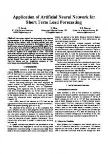
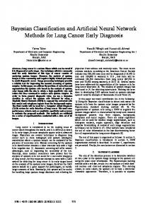
The idea behind the proposed technique is to replace all the active components in a complex external system by a recurrent ANN, which is connected to the same boundary buses. In addition, lumped equivalent loads are connected at the boundary nodes to account for the passive elements in the external area. The principles of the proposed dynamic equivalencing approach are explained in Fig. 1 for one boundary bus. Like any active component in the power system, the ANN is perturbed by the voltages at the boundary buses. The ANN reacts to the voltage changes by varying the injected currents to the boundary nodes. Currents (real and imaginary parts) are chosen as outputs from the ANN as they are found to give better convergence in the training process compared with the alternative active and reactive power. This behaviour is evident taking into consideration that the power represents the product of voltage and current. However, the voltage is already an input variable to the ANN. Thus, using current as the output from the ANN allows a better separation between the real inputs and outputs. In this case, the ANN will operate according to the principles of a Norton model. If the simulation software that is used works with injected power, it can be calculated outside the ANN as represented by the function (f2) in Fig. 1.
external area to be replaced by the recurrent ANN and the equivalent lumped passive elements
z −n .
.
.
U P, Q
U
internal area
ff1 ∆U n
P, Q
n
ANN
z −1
z −m
.
−2 . z
∆Ia
f2
Pa, Qa
Pp, Qp
passive elements
active elements
Fig. 1
Principles of the proposed dynamic equivalencing approach
To avoid developing a dynamic equivalent that is valid only for a certain initial power-flow condition, normalised 682
n ¼ DIa;i
DUin ¼
0 Ia;i � Ia;i 0 Ia;i
Ui � Ui0 Ui0
i ¼ 1; 2 . . . j
ð1Þ
i ¼ 1; 2; . . . j
ð2Þ
where: n DIa;i normalised deviation of complex current of the active components at boundary bus i, Ia,I complex current of the active components at boundary bus i, DUin normalised deviation of complex voltage at boundary bus i, Ui complex voltage at boundary bus i, 0 Ia;i ; Ui0 initial values of Ia,i and Ui respectively,
j number of boundary buses
z −2 z −1
.
internal area to be held unchanged
deviations rather than the variables themselves are used (1). Furthermore, the paper suggests describing passive loads of the external system separately as lumped elements at the boundary buses as shown in Fig. 1. This results in more flexibility and a general representation of the external system. The passive loads can also be considered to be as voltage and frequency dependent by common techniques. The portion of active elements is modelled separately by the recurrent ANN, where the ANN itself is a normalised per unit model scaled on the basis of actual conditions outside the ANN. This approach allows the same ANN model to be used even if the active and passive loading-conditions are changed inside the external system itself. This will help to obtain a generic dynamic equivalent unlike most known approaches. At each time interval, the instantaneous values of the boundary-bus voltages are used to compute the normalised voltage-deviations through the function (f1). The normalised voltage deviations are introduced to the equivalent model and processed with previous normalised current and voltage deviations to calculate the present normalised current deviations at each boundary bus using the ANN. The normalised deviations of current and voltage are computed based on their initial conditions using the following expressions:
Real and imaginary parts of DUin are used as separate inputs to the ANN, while the real and imaginary n are obtained as separate outputs from components of DIa;i the ANN. The actual values of the complex currents are calculated inside the function (f2) and supplied at the boundary buses. If necessary, the active and reactive powers can also be computed inside this function and conducted to the internal network as shown in Fig. 1. Although the ANN-based equivalent is not in a standard form like other elements in power systems, its simple configuration facilitates the implementation of this model within the power system simulation software. At the same time, simulating the equivalent model using modern computers is a very fast and simple task even if the ANN has many parameters. The utilisation of past values of currents and voltages as inputs to the ANN is essential to obtain a dynamic equivalent, whose order depends on the number of recurrent loops. When this feature is coupled with the nonlinear capability of the ANN, the resulting model will be able to model any external nonlinear dynamic system accurately. IEE Proc.-Gener. Transm. Distrib., Vol. 151, No. 6, November 2004
3
Test network 2
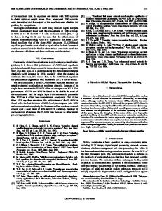
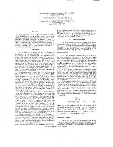
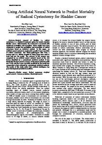
A 16-machine 380/220 kV network is used in this research to test and verify the proposed technique [12]. However, the network is extended by one 110 kV-system including the underlying 10 and 0.4 kV parts. This area is assumed to be the external network, which will be replaced by an equivalent dynamic model. On the other hand, the highvoltage system is modelled and simulated in detail and is assumed to be the internal system. The 110 kV section is shown in Fig. 2, where two interconnecting buses B1 and B2 represent the connection nodes to the high-voltage network. To extend the network to the low-voltage level, two steps of transformation are used (i.e. from 110 to 10 kV and then from 10 kV to 0.4 kV) starting from the six-110 kV buses shown in the area bounded by the dotted block. In the lowvoltage area, 56 fuel cells and 56 microturbines with different capacities are modelled and connected near to the end-user terminals. The DGU are connected to the load centres through 100–300 m cables.
3
DL 20 km
30 km
4 10 kV
20 km 20 km
5
110 kV
1
20 km 20 km MT
6
FC
FC
MT
MT
FC
0.4 kV
10 kV
10 kV
0.4 kV MT
FC
MT
FC
MT
FC
MT
FC
10 kV
B1
380 kV
high voltage network with 220 and 380 kV levels
0.4 kV MT
30 km
110 kV 20 km
20 km
FC
MT
FC
MT
FC
MT
FC
Buses 1–5 are extended to low-voltage area with similar integration to that shown for bus 6 FC fuel cell MT microturbines
20 km
20 km
MT
Fig. 3 Modelling the medium-and the low-voltage sections showing the integration of fuel cells and micro turbines into the end user terminals
300 MVA DL 20 km
FC
250 MVA
220 kV B2
Table 1: Summary of internal and external systems data Internal system
110 kV section with the underlying low-voltage distribution system to be replaced by the equivalent dynamic model
Fig. 2
110 kV area with boundary buses
110 kV section with underlying low-voltage distribution to be replaced by equivalent dynamic model
Figure 3 illustrates the structure of the medium-and low-voltage levels showing the integration of the DGU into the load centres starting from one 110 kV bus. Similar structures are used from the other five 110 kV buses. An investigation using the full model was introduced in work to highlight the interaction between the DGU and the high-voltage network [13]. The configuration of the distribution system and the detailed dynamic models of both the fuel cells and the microturbines are also, presented in [13]. Table 1 summarises the number of components in both the internal network and the external distribution system. Although the 110 kV system represents a small part of the entire network, the large number of components in this single distribution system considerably complicates the dynamic simulation. In real interconnected systems, where the number of elements in the distribution system reaches up to thousands of units, the detailed simulation of all elements will not be feasible. Conventionally, lumped-load representation is used for the general voltage and frequencydependant elements. IEE Proc.-Gener. Transm. Distrib., Vol. 151, No. 6, November 2004
External system
Buses
60
238
Branches
45
178
Transformers
26
64
Synchronous generators
16
0
Microturbines
0
56
Fuel cells
0
56
In the near future, the distributed sources may be used within power systems to generate a significant part of the network power [13]. In the network under consideration, the power from the active DGU reaches up to 30% of the total load demand in the low-voltage area. Therefore, the impact of such units on the dynamics of the high-voltage networks has to be considered. To assess the error due to neglecting this dynamic contribution, the performance of the entire network is investigated for three cases. First, the distribution system is modelled in detail with all DGU. Secondly, the conventional lumped representation is considered, where the equivalent load at each boundary bus depends only on the voltage at this bus with a general exponential relation. Finally, the power of the equivalent loads is related to the voltages at all boundary buses with 683
general exponential relations as follows: �� �p1;i � �p2;i � U1 U2 � Pi ¼ Pi0 i ¼ 1; 2 U10 U20 Qi ¼
Q0i
��
U1 U10
�q1;i � �q2;i � U2 � U20
i ¼ 1; 2
4 ð3Þ
ð4Þ
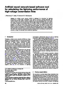
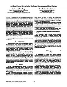
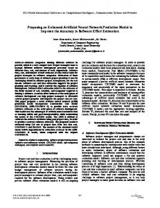
where:Pi and Pi0 are the active power at bus i and its initial value, Qi and Q0i and the reactive power at bus i and its initial value respectively, P1,i, P2,i, q1i are q2,i are coefficients. An optimisation process is carried out with the second and third cases to define the best values of the unknown coefficients by minimising the error between the actual and the calculated supplied powers. The minimisation of differences is carried out without restricting the coefficients to the known typical limits and therefore, the obtained coefficients have values in the range 720. This is intended to obtain the best possible performance. Figure 4 shows the powers transferred to the 110 kV area following a three-phase short-circuit in the internal system in the three cases. 80 70 60 50 40 30 20 10
a
30 25 20 15 10 5 0
b
5.1
0
5
time, s d
ANN-based dynamic equivalents
As is well known, ANNs are well able to deal with complicated nonlinear problems, as they can recognise and resimulate nonlinear mappings [10]. Another important characteristic of ANNs is their generalisation feature, which enables them to be successfully applied to new situations, which are not used in the training phase. Therefore, well trained recurrent ANNs can replace the complex distribution system and are expected to interact with the highvoltage network under any operating conditions.
c
10
15
original full system lumped load representation depending on voltages at all boundary buses lumped load representation depending on the voltage at the local node
Fig. 4 Performance of the original full-system and the two-lumped load-modelling approximations a active power at bus B1, MW b reactive power at bus B1, Mvar c active power at bus B2, MW d reactive power at bus B2, Mvar
It is obvious from Fig. 4 that this representation cannot be used to represent distribution systems include active sources. When the coefficients are restricted to the typical limits, worse results are obtained, which emphasises that it is not feasible to use this approximation. 684
The ANN proposed to represent all the active elements in the distribution network has been trained by time series. For this purpose, a number of three-phase short-circuits are simulated at different nodes in the internal network. In each case, the simulation is carried out for 15 s, which is enough to restore the steady-state conditions after the fault clearance. The modelling and simulation are accomplished using the Power system dynamics (PSD) simulation package [14]. Complex voltages, power transfer and injected currents all at the boundary buses are stored during the fault simulation. These results have then been used to prepare suitable patterns for ANN training. The passive loads in the distribution system are lumped at the two boundary buses and represented separately as constant-impedance elements. If passive loads have other characteristics, suitable equivalent representations can be developed in a general form depending on network voltages and frequency. As an alternative, the entire distribution system can also be replaced by the recurrent ANN if the information about the system is not enough to represent the passive loads separately. This can also be applied if the joint simultaneous impact of all boundary-bus voltage variations on the passive load is considered. However, in this case the recurrent ANN is restricted to a fixed ratio of active and passive components, which limits its applicability. 5
60 50 40 30 20 10 0
15 10 5 0 −5 −10 −15
Data preparation
ANN structure
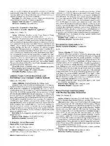
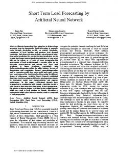
To extend the conventional feedforward ANN to the dynamic domain, a time history of the variables has to be involved in the input features to the network. The ANN has to capture dynamics from both the internal system (defined by the voltages as inputs to the ANN) and the external system (defined by currents as outputs from the ANN). Therefore, past values of both the normalised voltage and current deviations are used at the input layer of the ANN. In the investigated test case with two boundary buses, the ANN has 36 inputs and four outputs. The inputs to the ANN include the real and imaginary components of the normalised boundary-bus voltages at present and four previous time intervals. Real and imaginary components of normalised injected currents to boundary buses at four previous time intervals are also received at the input nodes of the network. The four outputs represent the real and imaginary components of normalised current deviations at the two boundary buses at the present time interval. Several neural networks with different structures are tested to obtain the best possible performance. The best accuracy is obtained from an ANN comprising two hidden layers with 50 and 20 neurons in the first and the second hidden layers respectively. In this network, all the neurons in the hidden layers have nonlinear sigmoid functions, while the output neurons have linear activation functions. The structure of the ANN is shown in Fig. 5. IEE Proc.-Gener. Transm. Distrib., Vol. 151, No. 6, November 2004
40 real and imaginary n components of ∆ U 1 at present and 4 previous time intervals
20 0 − 20 ANN
real and imaginary n components of ∆U 2 at present and 4 previous time intervals
real and imaginary n components of ∆Ia,1 at 4 previous time intervals
2 hidden layers with 50 and 20 neurons in the first and the second layers, respectively
real and imaginary n components of ∆Ia,1 at present time intervals
− 40 − 60
a
20 0 − 20 real and imaginary n components of ∆Ia,2 at present time intervals
real and imaginary n components of ∆Ia,2 at 4 previous time intervals
− 40
b
40 20 0 − 20 − 40
Fig. 5
Structure of the ANN
− 60
c
20
5.2
Training process
Patterns corresponding to eight different three-phase short circuits are used to train the ANN, while patterns corresponding to other four faults are kept for the test process. The total simulation time for each fault is 15 s with a 5 ms integration time step. This results in a total of 24,000 patterns used to train the ANN. In this study, the online back propagation-training algorithm is used, where the parameters are updated after each pattern has being processed. The training process is accomplished offline, where the prepared time-history variables are applied the input layer without real feedback loops. However, this is the case only in the training phase, real recurrent loops are used in the simulation process. Therefore, the evaluation of training and testing the ANN is based on the online simulation of the entire network including the ANN-based model with real feedback loops. 6
0 − 20 − 40
0
5
10
15
time, s d actual performance ANN-based equivalent
Fig. 6 Original and the equivalent systems under a disturbance used in training process a active power at bus B1, MW b reactive power at bus B1, Mvar c active power at bus B2, MW d reactive power at bus B2, Mvar
Simulation results and discussion
After training the ANN in the offline mode, it is tested under the same disturbances that are used in the training process, however, in the online mode recoupled outputs are used. Figure 6 shows a comparison between the complex power of the active units with the full model and with the ANN-based equivalent model. The disturbance is a threephase short-circuit in the 380 kV high-voltage system. The negative sign of the steady-state values of power in the Figures indicates that the power is flowing out from the active sources. The coincidence between the performances indicates that the ANN has learnt the nonlinear behaviour of the external system. However, it is necessary to test the system under new disturbances to examine the generalisability capability of the ANN. Therefore, Fig. 7 shows a comparison under a three-phase short-circuit at a 220 kV bus, was not used in the training process. The agreement between the two models is obvious, reflecting the ability of the ANN to generalise the dynamic characteristics of the external system. The developed model was also tested under several new disturbances, where the performance was always similar to that of the original full model. This ensures that of using the developed dynamic equivalent model can be used as an alternative to the complex full model under different perturbations inside the internal network. IEE Proc.-Gener. Transm. Distrib., Vol. 151, No. 6, November 2004
To examine the validity of the ANN-based model starting from new power-flow conditions, the loading conditions in the internal network are changed and a new power-flow analysis is carried out. The steady state powers of both active and passive elements in the external system are held constant under the new loading conditions. Table 2 summarises the steady-state values of the line voltages as well as the complex power transfer to the distribution system at each boundary bus for the base case and the new power flow condition. In large stable networks, such variations in the voltages and powers represent a significant change in the operating point. This can cause loss of accuracy if the equivalent model is not in a general form or is restricted to a certain operating point. Since the loading conditions in the external network are not changed, the total power transferred to the low-voltage network is not changed. The slight increase in the total power transferred accounts for the increase in the power loss due to the voltage reduction. Figure 8 shows a comparison between the power from active units at the two boundary buses using the full model and the ANN-based model following a three-phase short circuit at a 220 kV bus starting from the new initial conditions. Using the normalised deviations rather than this normalised variables or the variables themselves extends the validity of the dynamic equivalent to new initial conditions with high accuracy. 685
20
50
0
0
− 20
− 50
− 40
− 100
− 60
a
a
5
40
0
20
−5
0
− 10
− 20
− 15
− 40
− 20
b
b
20
100 50
0
0 − 20
− 50 − 100
− 40
c
c
0
20 0
− 10
− 20
− 20
− 40 − 60 0
5
10
15
− 30
0
5
10
time, s
time, s
d
d
actual performance
actual performance
ANN-based equivalent
ANN-based equivalent
15
Fig. 7 Original and the equivalent systems under a disturbance not used in training process
Fig. 8 Original and equivalent systems starting from a new powerflow initial condition
a active power at bus B1, MW b reactive power at bus B1, Mvar c active power at bus B2, MW d reactive power at bus B2, Mvar
a active power at bus B1, MW b reactive power at bus B1, Mvar c active power at bus B2, MW d reactive power at bus B2, Mvar
Table 2: Initial conditions for base and new power-flow cases
Table 3: New loading conditions of active units
U10 (kV)
U20 (kV)
S1 (MVA)
S2 (MVA)
Base case
381.15
222.53
54.82+j15.31
22.33+j3.26
New case
378.34
221.42
61.43+j13.41
15.84+j5.95
Modelling active components separately from the passive loads helps to develop a universal dynamic equivalent, which can represent the original system even with new loading conditions in the external system. Conventional dynamic equivalents will not be applicable if there is any change in the replaced system. Rather, a new dynamic model has to be developed to represent the external system under the new conditions. To emphasise this point, the power from active sources in the distribution system is decreased to about 50% of the original value by switching off some of these units. As a result, the contribution of active sources at each boundary bus is changed in Table 3. However, the power of the passive elements is held constant under the new conditions. After changing the loading conditions of the active units in the distribution system, a power-flow analysis is repeated 686
Power portion from active sources through boundary buses (MVA) through bus B1
through bus B2
Base case
15.86+j8.28
13.85+j9.29
New case
8.30+j4.24
7.57+j4.95
and a three-phase short-circuit is simulated at a 220 kV bus in the internal area. Figure 9 comparies the power of active units using the full model and the equivalent model following the abovementioned fault. The results show that the ANN-based model is still accurate under the new situation in the external system, although considerable change has occurred in the external network itself. To account for the new situations in the internal and/or the external networks, no modifications are introduced to the ANN-based dynamic model. Rather, the new conditions are simulated by modifying the initial conditions of currents and voltages in the functions (f1) and (f2) depending on the power-flow results. The integration time step used in the simulation after training the ANN and implementing the dynamic IEE Proc.-Gener. Transm. Distrib., Vol. 151, No. 6, November 2004
50
20 0
0
− 20
− 50
− 40 − 60
− 100
a
20
a
40 20 0
0
− 20 − 40
− 20
− 60
b
30
b
10 50
10
0 − 10
− 50
− 30
− 100
c
10
50
0
25
− 10
0
− 20
− 25
− 30
0
5
10
15
− 50
c
0
5
time, s d
10
15
time, s d 5 ms 10 ms 25 ms
actual performance ANN-based equivalent
Fig. 9 Original and equivalent systems under new loading conditions in distribution system
Fig. 10 ANN-based equivalent model under three different integration time steps
a active power at bus B1, MW b reactive power at bus B1, Mvar c active power at bus B2, MW d reactive power at bus B2, Mvar
a active power at bus B1, MW b reactive power at bus B1, Mvar c active power at bus B2, MW d reactive power at bus B2, Mvar
equivalent in the simulation software represents another important issue about the proposed technique. As the ANN is trained by data prepared using a certain integration time step, results at other simulation time steps have to be verified to evaluate the effect of varying the integration time step on the results. Figure 10 comparies the power from active units using the ANN-based equivalent using three different integration time steps after simulating a threephase short-circuit at a 380 kV bus. The three integration time steps are 5 ms, which is the integration time step used in the training process, 10 ms and 25 ms. Even with a large difference between the used integration time step and that used in the training process, the performance is still in agreement with the original case, which is given by the curve at 5 ms. Depending on the comparison illustrated in Fig. 10, it is possible to simulate the network including the ANNbased model with different integration time steps with acceptable accuracy. However, using an integration time step, which is equal or close to that used in the training process, will ensure higher accuracy.
new initial conditions even after variations in the external system itself. Due to the separate representation of active and passive parts of the system, it is also applicable when changing the contribution of active distribution units in covering the local demand. Another advantage of the ANN-based equivalent is that only variables at the boundary buses are needed for the training process. Thus, it can also be trained with time series that have been recorded in real systems. Furthermore, the model is not restricted to the integration time step used for training the ANN. All simulation results show a very good aggreement between the detailed and the ANN-based equivalent model. In general, the results encourage the use of ANN-based dynamic equivalens especially for distribution systems when the portion of DGUs increases. However, it requires the implementation of ANNs into power system dynamic simulation software.
7
Conclusions
A new approach has been introduced in this paper has been to identify suitable dynamic equivalents to distribution systems, which contain a large number of active sources, based on recurrent ANNs. A main advantage of the proposed method is its universality as it is still valid under IEE Proc.-Gener. Transm. Distrib., Vol. 151, No. 6, November 2004
8
References
1 Kim, J.Y., Won, D.J., and Moon, S.I.: ‘Development of the dynamic equivalent model for large power system’. Proc. IEEE. Power Engineering Society Summer Meeting IEEE, Vancouver, Canada, 2001, Vol. 2, pp. 973–977 2 Price, W.W., Hargrave, A.W., Hurysz, B.J., Chow, H.J., and Hirsch, P.M.: ‘Large-scale system testing of a power system dynamic equivalencing program’, IEEE Trans. Power Syst., 1998, 13, (3), pp. 768–774 3 Wang, L., Klein, M., Yirga, S., and Kundur, P.: ‘Dynamic reduction of large power systems for stability studies’, IEEE Trans. Power Syst., 1997, 12, (2), pp. 889–895 687
4 Ju, P., and Zhou, X.Y.: ‘Dynamic equivalents of distribution systems for voltage stability studies’, IEE Proc. Gener. Transm. Distrib., 2001, 148, (1), pp. 49–53 5 Galarza, R.J., Chow, J.H., Price, W.W., Hargrave, A.W., and Hirsch, P.M.: ‘Aggregation of exciter models for constructing power system dynamic equivalents’, IEEE Trans. Power Syst., 1998, 13, (3), pp. 782–788 6 Demmig, S., Pundt, H.H., and Erlich, I.: ‘Identification of external system equivalents for power system stability studies using the software package MATLAB’. Presented at 12th power systems computation conference, Dresden, Germany, 1996 7 Nojiri, K., Suzaki, S., Takenaka, K., and Goto, M.: ‘’Modal reduced dynamic equivalent model for analog type power system simulator’, IEEE Trans. Power Syst., 1997, 12, (4), pp. 1518–1523 8 Joo, S.K., Liu, C.C., and Choe, J.W.: ‘Enhancement of coherency identification techniques for power system dynamic equivalents’. Presented at IEEE PES Summer Meeting, Vancouver, Canada, 2001
688
9 Joo, S.K., Liu, C.C., Jones, L., and Choe, J.W.: ‘Coherency techniques for dynamic equivalents incorporating rotor and voltage dynamics’. Presented at Conf. on bulk power systems dynamics and control – V, security and reliability in a changing environment, Hiroshima, Japan, August 2001 10 Wang, M.H., and Chang, H.C.: ‘Novel clustering method for coherency identification using an artificial neural network’, IEEE Trans. Power Syst., 1994, 9, (4), pp. 2056–2062 11 Miah:, A. M.: ‘Simple dynamic equivalent for fast online transient stability assessment’, IEE Proc. Gener. Transmi. Distrib., 1998, 145, (1), pp. 49–55 12 Test network, PST16, http://www.uni-duisburg.de/FB9/EAN/doku/ teeuwsen/PST16.html 13 Azmy, A.M., and Erlich, I.: ‘Dynamic simulation of fuel cells and micro-turbines integrated with a multi-machine network’. Presented at IEEE Bologna Power Tech Conf., Bologna, Italy, 2003 14 Erlich, I.: ‘Analysis and simulation of dynamic behavior of power system’. Postdoctoral thesis, Technical University of Dresden, Germany, 1995
IEE Proc.-Gener. Transm. Distrib., Vol. 151, No. 6, November 2004