Corresponding Author: K. K. Pradhan, Vikash School of Business Management,. Bargarh, Odisha, India. Artificial Neural Network Methodology for Modeling and ...
International Journal of Creative Mathematical Sciences & Technology (IJCMST) 2(1): 35-41, 2012
ISSN (P): 2319 – 7811, ISSN (O): 2319 – 782X
Artificial Neural Network Methodology for Modeling and Resource use Optimization in Rice Yield K. K. Pradhan1, S. K. Hota2 and B. Satpathy3 1
Vikash School of Business Management, Bargarh (Odisha), India Madhusudan Institute of Cooperative Management, Bhubaneswar (Odisha), India 3 Sambalpur University, Jyoti Vihar Burla (Odisha), India
2
Abstract: “Artificial neural networks (ANN)”, viz. Multilayer Perceptron (MLP) using Neuro Solutions 5.0 having 2 numbers of Hidden Layers and 50 Neurons per Hidden Layer has been used here to predict the inputs for a given value of output. Another artificial neural network viz. Radial Basic Function (RBF) using SPSS 17.0 that typically have three layers: an input layer, a hidden layer with a non-linear RBF activation function and a linear output layer has also been used in this paper for modeling the resource use optimization problem. The paper has illustrated the optimization problem by considering rice crop yield data as the output (Y) and per acre Cost of Bullock/ Machine Labor (X1), Human labor (X2), Seeds (X3), Fertilizer (X4), Irrigation (X5), Pesticide (X6) and Credit (X7) as inputs. It has been observed that for a desired level of output the input costs predicted by RBF is better than MLP for the data considered in this study. It is hoped that, in future, research workers would start applying these advanced ANN models to optimization problems relating to agricultural productivity. Keywords: ANN, RBF, Optimization.
INTRODUCTION Multiple linear regression modeling is widely used to estimate linear relationship between response variable and predictors. Its limitation is that it assumes the underlying relation between response and predictor variables to be “linear”. In real life situation, this assumption is rarely satisfied. Also, if there are several predictors, it is quite impossible to have an idea of the underlying non-linear functional relationship between response and predictor variables. To handle such a situation, “Artificial neural networks” (ANNs) is used. Cheng and Titterington (1994) have reviewed the ANN methodology from a statistical perspective, while Warner and Misra (1996) have laid emphasis on the understanding of ANN as a statistical tool. A distinguishing feature of ANNs that makes them valuable and attractive for a statistical task is that, as opposed to traditional model-based methods, ANNs are data-driven self-adaptive methods in that there are a few a-priori assumptions about the models for problems under study. This modeling approach with ability to learn from experience is very useful in many practical problems since it is often easier to have data than to have good theoretical guesses about the underlying laws governing the systems from which data are generated. Zhang (2007) has discussed various pitfalls in the ANN modeling work, which must be avoided. Most widely used ANN is multilayered feed forward artificial neural network (MLFANN). 35 Corresponding Author: K. K. Pradhan, Vikash School of Business Management, Bargarh, Odisha, India
International Journal of Creative Mathematical Sciences & Technology (IJCMST) 2(1): 35-41, 2012
ISSN (P): 2319 – 7811, ISSN (O): 2319 – 782X
In this paper an attempt has been made to solve a resource use optimization problem relating to the cultivation of rice by taking the field data from the small farmers of a village situated in the Bargarh district of western Odisha in India. We have used two different types of neural networks namely a Time-Lagged Feed forward Network (TLFN) and a Radial Basic Function (RBF) Network to compare the results. Here Neuro Solutions 5.0 and SPSS 17.0 software have been used to build the networks respectively. Neuro Solutions 5.0 neural network uses Time-Lagged Feed forward Network (TLFN). It is a Multi-Layer Perceptron (MLP) with memory components to store past values of the data in the network. The memory components allow the network to learn relationships over time. It is the most common temporal supervised neural network. It consists of multiple layers of Processing Elements (PEs) connected in a feed forward fashion. Neuro Solutions uses the back-propagation of errors to train the MLP. The back-propagation uses gradient search and adjust the weights contained in the network. This is how the network is trained. The selected network has been constructed with two hidden layers. The analysis has been undertaken with 1000 epochs. An epoch is a complete presentation of the training data to the network. In this analysis a Prediction type problem analysis has been made. Prediction problems are those where the goal is to determine an output given a set of inputs and the past history of the inputs. The main difference between prediction problems and the others is that prediction problems use the current input and previous inputs (the temporal history of the input) to determine either the current value of the output or a future value of a signal. The target of a MLP is learning to match a vector of inputs (X) to a vector of outputs (Y) through the interactions among neurons (W). This implies learning the function. Through the sample {X(p), Y(p)}, p = 1,2,…,N where x( p) R n is the input vector and y ( p) R m is the output, where i denote input, j hidden and k output layer. f
Rn Rm f (W : X ) ~ Y y k f 0 wik xi i k
w j k
jk
f h wij xi -----------------------(1) i j
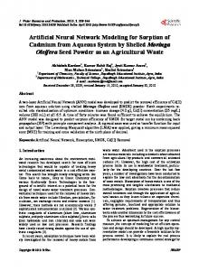
This is carried out by adjusting the weights (W) of given interconnections according to some learning algorithm. MLP employs a supervised learning algorithm called back propagation. The learning is guided by specifying the desired response to the network for each training input pattern through the comparison with the actual output computed by the network in order to adjust the weights. These adjustments have the purpose of minimize some energy function, normally the square difference between the desired and actual outputs. The derivatives of the function with respect to the weights are employed to propagate the error backwards through the network from output to hidden layer(s), until it reaches the input layer. Each weight is modified according with its particular contribution to the global error. The performance of the net is measured most of times in terms of the root mean square error. After a number of loops, when the benefits of further optimization are regarded as small, the training process converges and stops. A typical MLP Architecture has been shown below. 36 Corresponding Author: K. K. Pradhan, Vikash School of Business Management, Bargarh, Odisha, India
International Journal of Creative Mathematical Sciences & Technology (IJCMST) 2(1): 35-41, 2012
ISSN (P): 2319 – 7811, ISSN (O): 2319 – 782X
Multilayer Perception Architecture
RADIAL BASIS FUNCTION (RBF) A Radial Basis Function (RBF) is a real-valued function whose value depends only on the distance from the origin, so that
; or alternatively on the distance from . Any function φ that
some other point c, called a center, so that
satisfies the property is a radial function. The norm is usually Euclidean distance, although other distance functions are also possible. According to Lukaszyk (2004) by using Lukaszyk-Karmowski metric it is possible to avoid problems with ill conditioned matrix for some radial functions and also we can determine coefficients wi since the is always greater than zero. Sums of radial basis functions are typically used to approximate given functions. This approximation process can also be interpreted as a simple kind of neural network. Commonly
used types of radial basis functions include r x c i :
Gaussian: ( r ) exp( r 2 ) for some 0 .
Multiquadric: (r )
rk k 1,3,5,... Polyharmonic spline: ( r ) k r ln( r ) k 2,4,6,...
Thin plate spline (a special polyharmonic spline): ( r ) r 2 ln( r )
r 2 2 for some 0 .
Radial Basis Functions are typically used to build up function approximations of the form n
y ( x) wi x ci
i 1
where the approximating function y(x) is represented as a sum of N radial basis functions, each associated with a different center ci, and weighted by an appropriate coefficient wi. The weights wi can be estimated using the matrix methods of linear least squares, because the approximating function is linear in the weights. 37 Corresponding Author: K. K. Pradhan, Vikash School of Business Management, Bargarh, Odisha, India
International Journal of Creative Mathematical Sciences & Technology (IJCMST) 2(1): 35-41, 2012
ISSN (P): 2319 – 7811, ISSN (O): 2319 – 782X
The sum can also be interpreted as a rather simple single-layer type of artificial neural network called a radial basis function network, with the radial basis functions taking on the role of the activation functions of the network. It can be shown that any continuous function on a compact interval can in principle be interpolated with arbitrary accuracy by a sum of this form, if a sufficiently large number N of radial basis functions is used. n
y ( x) wi x ci
i 1
The approximant y(x) is differentiable with respect to the weights wi. The weights could thus be learned by using any of the standard iterative methods for neural networks.
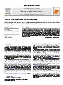
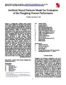
METHODOLOGY RESULTS AND CONCLUSION The present study aims at using ANN as a tool to solve resource use optimization problems. As an illustration, the methodology has been applied for modeling and forecasting of rice crop yield on the basis of seven variables. We have taken rice crop yield data as the output (Y) and Total Cost of Bullock/ Machine Labor-per acre (X1), Total Cost of Human Labor per acre (X2), Cost of Seeds per acre (X3), Fertilizer cost per acre (X4), Total-Irrigation Cost (X5), Cost of pesticide (X6) and Credit per acre (X7) as different inputs. The network information regarding the RBF using SPSS 17.0 has been shown in the Table 1. Overall Percent Correctness during training of the data is found to be 15.5%. Training Time required was 0:00:05.657. The Primary data has been collected through personal interview method based on a pre-designed questionnaire from 84 numbers of small farmers of a village situated in the Bargarh district of Odisha. The poor record keeping system existing among the farmers is one of the main constraints to this kind of research where the farmers have given data from their memory. We trained the data and we changed our data set and assigned zero value to X1, X2, X3, X4, X5, X6 and X7 with a targeted level of output and we ran the network to get the values of Xi (where i = X1….. X7). For example, we fixed the target to be 7106 Rupees and we got the X1, X2, X3, X4, X5, X6 and X7 values in Rupees that has been shown in the Figure-1 as well as in the Table-3. The same thing was repeated for running the Neuro Solution 5.0 and SPSS 17.0 software. The Figure-1 shows the comparative result of SPSS 17.0, Neuro Solutions 5.0 and the actual data gathered from the farmers. The Network Information and the Case processing summary for SPSS 17.0 using MLP network have been shown in the Table 2 and 3. The cumulative mean square error in case of Neuro Solutions 5.0 was found to be 0.1075. The number of epochs was found to be 1000. Neuro Solutions 5.0 neural network used Time-Lagged Feed forward Network (TLFN) with two hidden layers. To know the difference between the predictions we used two cases where the target was Rs. 6847.6 but the primary data were different. We found that the SPSS 17.0 predicted the same value for both the cases while the Neuro Solutions 5.0 gave different values which have been depicted in Graph 2 and 3 and also in Table 3. Therefore to our view the Neuro Solutions 5.0 is giving better result by taking care of the primary data and predicting the values while the SPSS 17.0 is only considering the target value given which is the input in this case for the Networks. Evidently, predicted and actual values in both the methods i.e RBF and MLP are quite close. 38 Corresponding Author: K. K. Pradhan, Vikash School of Business Management, Bargarh, Odisha, India
International Journal of Creative Mathematical Sciences & Technology (IJCMST) 2(1): 35-41, 2012
ISSN (P): 2319 – 7811, ISSN (O): 2319 – 782X
The neural network results show that the total cost human labor. /Ac. in RS. X2 is to be reduced and cost towards the irrigation facilities X5 is to be increased. The result seems to be practical since the labor cost is high and the farmers should invest more in irrigation for better productivity. Thus, it could be concluded that artificial neural network methodology is successful in describing the given data and can be used as a reliable tool for resource use optimization problems. Table 1 Network Information using SPSS 17.0 Input Layer
Factors
1
Hidden Layer
Output_Y
Number of Units
46
Number of Units
2a
Activation Function Softmax Output Layer
Dependent Variables 1
Bullock_X1
2
Humane_X2
3
Seeds_X3
4
Fertilizer_X4
5
Irrigation_X5
6
Pesticide_X6
7
Credit_X7
Number of Units
271
Activation Function
Identity
Error Function
Sum of Squares
a. Determined by the Bayesian Information Criterion: The "best" number of hidden units is the one that yields the smallest BIC in the training data.
Table 2 Case Processing Summary using SPSS 17.0 N Sample
60
100.0%
Valid
60
100.0%
Excluded
44
Total
Training
Percent
104
39 Corresponding Author: K. K. Pradhan, Vikash School of Business Management, Bargarh, Odisha, India
International Journal of Creative Mathematical Sciences & Technology (IJCMST) 2(1): 35-41, 2012
ISSN (P): 2319 – 7811, ISSN (O): 2319 – 782X
Table 3 Predicted Data by NeuroSolutions 5.0, SPSS 17.0 and the Original Data Y
X1
X2
X3
X4
X5
X6
X7
MLP Predicted Values (Neuro Solutions 5.0 ) 7106 6847.6 6847.6
572.65 580.15 581.74
1387.08 1436.32 1446.8
7106 6847.6 6847.6
530 540 540
1200 940 940
303.54 663.01 433.3 306.17 673.24 446.85 306.77 675.42 449.74 RBF Predicted Values(SPSS 17.0) 287.5 700 250 580 250 580 Original Data
394.65 263.1 263.1
214.06 202.67 200.24
803.81 793.26 791.01
214.29 250 250
642.86 750 750
7106 500 1600 270 670 131.55 260 666.67 6847.6 520 1600 248 760 131.55 280 500 6847.6 520 1680 260 720 131.55 240 400 Note: The value of output (Y) and inputs (X1 to X7) are measured in Rupees (Rs.) term. For a Target Output of Rs.7106 1800 1600
Valuesin Rs.
1400 1200
Neuro Solutions
1000
SPSS(RBF)
800
Original
600 400 200 0 X1
X2
X3
X4
X5
X6
X7
Inputs
Figure-1 For a Tar ge t Output of Rs.6847.6 1800 1600
ValuesinRs.
1400 1200 Neuro Solutions
1000
SPSS(RBF) 800
Original
600 400 200 0 X1
X2
X3
X4
X5
X6
X7
Inputs
Figure- 2 40 Corresponding Author: K. K. Pradhan, Vikash School of Business Management, Bargarh, Odisha, India
International Journal of Creative Mathematical Sciences & Technology (IJCMST) 2(1): 35-41, 2012
ISSN (P): 2319 – 7811, ISSN (O): 2319 – 782X For a Target Output of Rs.6847.6 1800 1600
ValuesinR s.
1400 1200 Neuro Solutions
1000
SPSS(RBF)
800
Original
600 400 200 0 X1
X2
X3
X4
X5
X6
X7
Inputs
Figure- 3
REFERENCES [1]. [2]. [3]. [4]. [5]. [6].
[7]. [8].
Buhmann, Martin D. (2003), Radial Basis Functions: Theory and Implementations, Cambridge University Press, ISBN 978-0-521-63338-3. Cheng, B. and Titterington, D. M. (1994). Neural networks: A review from a statistical perspective. Statistical Science, 9: 2-54. Cybenko, G. (1989). Approximation by superpositions of a sigmoidal function. Mathematics of Control, Signals and Systems, 2: 303-14. Hertz, J., Krogh, A. and Palmer, R.G. (1991). Introduction to the Theory of Neural Computation. Reading, MA: Addison-Wesley. Lukaszyk, S. (2004) A new concept of probability metric and its applications in approximation of scattered data sets. Computational Mechanics, 33, 299-3004. Singh, R. K., and Prajneshu (2008). Artificial Neural Network Methodology for Modeling and Forecasting Maize Crop Yield, Agricultural Economics Research Review, 21: 5-10. Warner, B. and Misra, M. (1996). Understanding neural networks as statistical tools. American Statistician, 50: 284-93. Zhang, G. P. (2007). Avoiding pitfalls in neural network research. IEEE Transactions on Systems, Man and Cybernetics— Part C: Applications and Reviews, 37: 3-16. ____________________
41 Corresponding Author: K. K. Pradhan, Vikash School of Business Management, Bargarh, Odisha, India