Artificial Neural Network Reduction Through Oracle Learning Joshua E. Menke∗and Tony R. Martinez† Department of Computer Science Brigham Young University Provo, UT 84604
[email protected],
[email protected]
Abstract Often the best model to solve a real-world problem is relatively complex. This paper presents oracle learning, a method using a larger model as an oracle to train a smaller model on unlabeled data in order to obtain (1) a smaller acceptable model and (2) improved results over standard training methods on a similarly sized smaller model. In particular, this paper looks at oracle learning as applied to multi-layer perceptrons trained using standard backpropagation. Using multi-layer perceptrons for both the larger and smaller models, oracle learning obtains a 15.16% average decrease in error over direct training while retaining 99.64% of the initial oracle accuracy on automatic spoken digit recognition with networks on average only 7% of the original size. For optical character recognition, oracle learning results in neural networks 6% of the original size that yield a 11.40% average decrease in error over direct training while maintaining 98.95% of the initial oracle accuracy.
1
Introduction
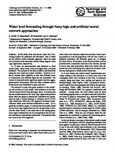
As Le Cun, Denker, and Solla observed in [14], often the best artificial neural network (ANN) to solve a realworld problem is relatively complex. They point to the large ANNs Waibel used for phoneme recognition in [21] and the ANNs of Le Cun et al. with handwritten character recognition in [13]. “As applications become more complex, the networks will presumably become even larger and more structured” [14]. The following research presents the oracle learning algorithm, a training method that takes a large, highly accurate ANN and uses it to create a new ANN which is (1) much smaller, (2) still maintains an acceptable degree of accuracy, and (3) provides improved results over standard training methods (figure 1). Designing an ANN for a given application requires first determining the optimal size for the ANN in terms of accuracy on a test set, usually by increasing its size until there is no longer a significant decrease in error. Once found, this preferred size is often relatively large for more complex problems. One method to reduce ANN size is to just train a smaller ANN using standard methods. However, using ANNs smaller than the optimal size results in a decrease in accuracy. The goal of oracle learning is to create smaller ANNs that are more accurate than can be directly obtained using standard training methods. ∗ http://axon.cs.byu.edu/ † http://axon.cs.byu.edu/∼martinez
1
Initial high accuracy model
Oracle Learning
Much smaller model which closely approximates the initial model
Figure 1: Using oracle learning to reduce the size of an ANN.
As an example consider designing an ANN for optical character recognition in a small, hand-held scanner. The ANN has to be small, fast, and accurate. Now suppose the most accurate digit recognizing ANN given the available training data has 2048 hidden nodes, but the resources on the scanner allow for only 64 hidden nodes. One solution is to train a 64 hidden node ANN using standard methods, resulting in a compromise of significantly reduced accuracy for a smaller size. This research demonstrates that applying oracle learning to the same problem results in a 64 hidden node ANN that does not suffer from nearly as significant a decrease in accuracy. Oracle learning uses the original 2048 hidden node ANN as an oracle to create as much training data as necessary using unlabeled character data. The oracle labeled data is then used to train a 64 hidden node ANN to exactly mimic the outputs of the 2048 hidden node ANN. The results in section 5 show the oracle learning ANN retains 98.9% of the 2048 hidden node ANN’s accuracy on average, while being 3.13% of the size. The resulting oracle-trained network (OTN) is 17.67% more accurate on average than the standard trained 64 hidden node ANN. Although the previous example deals exclusively with ANNs, both the oracle model and the oracle-trained model (OTM) can be any machine learning model (e.g. an ANN, a nearest neighbor model, a bayesian learner, etc.) as long as the oracle model is a functional mapping f : Rn → Rm where n is the number of inputs to both the mapping and the OTM, and m is the number of outputs from both. The same unlabeled data is fed into both the oracle and the OTM, and the error used to train the OTM is the oracle’s output minus the OTM’s output. Thus the OTM learns to minimize its differences with the oracle on the unlabeled data set. The unlabeled data set must be drawn from the same distribution that the smaller model will be used to
2
classify. How this is done is discussed in section 3.2. Since the following research uses multilayer feed-forward ANNs with a single-hidden layer as both oracles and OTMs, the rest of the paper describes oracle learning in terms of ANNs. An ANN used as an oracle is referred to as an oracle ANN (a standard backpropagation trained ANN used as an oracle). Oracle learning can be used for more than just model size reduction. An interesting area where we have already obtained promising results is approximating a set of ANNs that are “experts” over specific parts of a given function’s domain. A common solution to learning where there are natural divisions in a function’s domain is to train a single ANN over the entire function. This single ANN is often less accurate on a given sub-domain of the function than an ANN trained only on that sub-domain. The ideal would be to train a separate ANN on each natural division of the function’s domain and use the appropriate ANN for a given pattern. Unfortunately, it is not always trivial to determine where a given pattern lies in a function’s domain. We propose the bestnets method which uses oracle learning to reduce the multiple-ANN solution to a single OTN. Each of the original ANNs is used as an oracle to label those parts of the training set that correspond to that ANN’s “expertise.” The resulting OTN attemps to achieve similar performance to the original set of ANNs without needing any preprocessing to determine where a given pattern lies in the function’s domain. One application to which we have succesfully applied the bestnets method is to improve accuracy when training on data with varying levels of noise. Section 5.4 gives initial results on an experiment with clean and noisy optical character recognition (OCR) data. The results show that the bestnets-trained ANN is statistically more accurate than an ANN trained directly on the entire function. The resulting p-value is less than 0.0001—meaning the test is more than 99% confident that the bestnets-trained ANN is more accurate than the ANN trained on the entire function.
2
Background
Three research areas related to oracle learning are: 1. Model Approximation 2. Decreasing ANN Size 3. Use of Unlabeled Data The idea of approximating a model is not new. Domingos used Quinlan’s C4.5 decision tree approach from [19] in [10] to approximate a bagging ensemble [3] and Zeng and Martinez used an ANN in [22] to approximate a similar ensemble [3]. Craven and Shavlik used a similar approximating method to extract
3
rules [7] and trees [8] from ANNs. Domingos and Craven and Shavlik used their ensembles to generate training data where the targets were represented as either being the correct class or not. Zeng and Martinez used a target vector containing the exact probabilities output by the ensemble for each class. The following research also uses vectored targets similar to Zeng and Martinez since Zeng’s results support the hypothesis that vectored targets “capture richer information about the decision making process . . . ” [22]. While previous research has focused on either extracting information from ANNs [7, 8] or using statistically generated data for training [10, 22], the novel approach presented here is that available, unlabeled data be labeled using the more accurate model as an oracle. One goal of oracle learning is to produce a smaller ANN. Pruning [20] is another method used to reduce ANN size. Section 5.3 presents detailed results of comparing oracle learning to pruning for reducing ANN size. The results show that pruning is less effective than oracle learning in terms of both size and accuracy. In particular, oracle learning is more effective when reducing an initial model to a specified size. Much work has recently been done using unlabeled data to improve the accuracy of classifiers [2, 17, 16, 12, 1]. The basic approach, often known as semi-supervised learning or boot-strapping, is to train on the labeled data, classify the unlabeled data, and then train using both the original and the relabeled data. This process is repeated multiple times until generalization accuracy stops increasing. The key differences between semi-supervised and oracle learning are enumerated in section 3.4. The main difference stems from the fact that semi-supervised learning is used to improve accuracy whereas oracle learning is used for model size reduction.
3
Oracle Learning: 3 Steps
3.1
Obtaining the Oracle
The primary component in oracle learning is the oracle itself. Since the accuracy of the oracle ANN directly influences the performance of the final, smaller ANN, the oracle must be the most accurate classifier available, regardless of complexity (number of hidden nodes). In the case of ANNs, the most accurate classifier is usually the largest ANN that improves over the next smallest ANN on a validation set. The only requirement is that the number and type of the inputs and the outputs of each ANN (the oracle and the OTN) match. Notice that by this definition of how the oracle ANN is chosen, any smaller, standard-trained ANN must have a significantly lower accuracy. This means that if a smaller OTN approximates the oracle such that their differences in accuracy become insignificant, the OTN will have a higher accuracy than any standard-trained ANN of its same size—regardless of the quality of the oracle.
4
Note that the oracle should be chosen using a validation (hold-out) set (or similar method) in order to prevent over-fitting the data with the more complex model. As stated above, we chose the most accurate ANN improving over the next smallest ANN on a validation or hold-out set in order to prevent the larger ANN from overfitting.
3.2
Labeling the Data
The key to the success of oracle learning is to obtain as much data as possible that ideally fits the distribution of the problem. There are several ways to approach this. In [22], Zeng and Martinez use the statistical distribution of the training set to create data. However, the complexity of many applications makes accurate statistical data creation very difficult since the amount of data needed increases exponentially with the dimensionality of the input space. Another approach is to add random jitter to the training set according to some (a Gaussian) distribution. However, early experiments with the jitter approach did not yield promising results. The easiest way to fit the distribution is to have more real data. In many problems, like automatic speech recognition (ASR), labeled data is difficult to obtain whereas there are more than enough unlabeled real data that can be used for oracle learning. The oracle ANN can label as much of the data as necessary to train the OTN and therefore the OTN has access to an arbitrary amount of training data distributed as they are in the real world. To label the data, this step creates a target vector tj = t1 . . . tn for each input vector xj where each ti is equal to the oracle ANN’s activation of output i given the j th pattern in the data set, xj . Then, the final oracle learning data point contains both xj and tj . In order to create the labeled training points, each available pattern xj is presented as a pattern to the oracle ANN which then returns the output vector t j . The final oracle learning training set then consists of the pairs x1 t1 . . . xm tm for all m of the previously unlabeled data points. Therefore, the data are labeled with the exact outputs of the oracle instead of just using the class information. We found in earlier experiments that using the exact outputs yielded better accuracy than using only the class information. Current research is invesigating the cause of this improvement.
3.3
Training the OTN
For the final step, the OTN is trained using the data generated in step 2, utilizing the targets exactly as presented in the target vector. The OTN interprets each real-valued element of the target vector t j as the correct output activation for the output node it represents given xj . The back-propagated error is therefore ti − oi where ti is the ith element of the target vector tj (and also the ith output of the oracle ANN) and oi
5
is the output of node i. This error signal causes the outputs of the OTN to approach the target vectors of the oracle ANN on each data point as training continues. As an example, the following vector represents the output vector o for the given input vector x of an oracle ANN and o ˆ represents the output of the OTN. Notice the 4th output is the highest and therefore the correct one as far as the oracle ANN is concerned.
o = h0.27, 0.34, 0.45, 0.89, 0.29i
(1)
Now suppose the OTN outputs the following vector:
o ˆ = h0.19, 0.43, 0.3, 0.77, 0.04i
(2)
The oracle-trained error is the difference between the target vector in 1 and the output in 2:
o−o ˆ = h0.08, −0.09, 0.15, 0.12, 0.25i
(3)
In effect, using the oracle ANN’s outputs as targets for the OTN makes the OTN a real-valued function approximator learning to behave like its oracle. The size of the OTN is chosen according to the given resources. If a given application calls for ANNs no larger than 32 hidden nodes, then a 32 hidden node OTN is created. If there is room for a 2048 hidden node network, then 2048 hidden nodes is preferable. If the oracle itself meets the resource constraints, then, of course, it should be used in place of an OTN.
3.4
Oracle Learning Compared to Semi-supervised Learning
As explained in section 2, the idea of labeling unlabeled data with a classifier trained on labeled data is not new [2, 17, 16, 12, 1]. These semi-supervised learning methods differ from oracle learning in that: 1. With oracle learning the data is relabeled with the oracle’s exact outputs, not just the class. Preliminary experimentation showed using the exact outputs yielded improved results over using only the class information. In addition, Zeng and Martinez [22] show improved results using exact outputs when approximating with ANNs. We conjecture in section 5.2 that the improvement in accuracy comes because using the exact outputs creates a function solving the same classification problem that is easier to approximate using the backpropagation algorithm. Caruana proves this is possible in his work on RankProp [4, 5, 6]. 6
2. With oracle learning the relabeled data is used to train a smaller model, not the original oracle. In [2], Blum and Mitchell use co-training to improve the accuracy of two models trained on different “views” of the data. Each model trains on labeled data from one view of the data, and then labels unlabeled data for the other model. This is similar to oracle learning in that one model trains on labeled data and then labels unlabeled data for a different model to use, but it is different in three ways. First, with oracle learning both models use the same view of the data. In fact, the original labeled data used to train the oracle us relabeled for the OTM or OTN, and therefore the OTN sees a superset of the data used to train the oracle. The second difference is that in co-training, the each model is used to train the other, whereas in oracle learning, the OTM or OTN is not used to train the larger oracle. Finally, the goal of oracle learning is to reduce the size of the oracle, not to improve overall accuracy. Co-training seeks to improve accuracy on the problem through using an enhanced version of standard semi-supervised learning methods. 3. Oracle trained models can not over-fit the data. They attempt to overfit their oracles, allowing for less contrained learning. We submit that is may be indeed possible for a smaller OTN to fit its more complex oracle if the exact outputs from the oracle used for training the smaller ANNs produce a function that is easier to approximate than the original function when using backpropagation. Semi-supervised learning could be used as an oracle selection mechanism since it seeks to increase accuracy, but it not does not compare directly with oracle learning as used for model size reduction.
4
Methods
The following experiments serve to validate the effectiveness of oracle learning, demonstrating the conditions under which oracle learning best accomplishes its goals. Trends based on increasing the relative amount of oracle-labeled data are shown by repeating each experiment using smaller amounts of hand-labeled data while keeping the amount of unlabeled data constant. Further experiments to determine the effects of removing or adding to the unlabeled data set while keeping the amount of hand-labeled data constant will be conducted as subsequent research because of the amount of time required to do them.
4.1
The Applications
One of the most popular applications for smaller computing devices (e.g. hand-held organizers, cellular phones, etc.) and other embedded devices is automated speech recognition ASR. Since the interfaces are limited in smaller devices, being able to recognize speech allows the user to more efficiently enter data. 7
Given the demand for and usefulness of speech recognition in systems lacking in memory and processing power, there is a need for smaller ASR ANNs capable of achieving acceptable accuracy. One of the problems with the ASR application is an element of indirection added by using a phonemeto-word decoder to determine accuracy. It is possible that oracle learning does well on problems with a decoder and struggles on those without. Therefore, a non-decoded experiment is also conducted. A popular application for ANNs is optical character recognition (OCR) where ANNs are used to convert images of typed or handwritten characters into electronic text. Although unlabeled data is not as difficult to obtain for OCR, it is a complex, real-world problem, and therefore good for validating oracle learning. It is also good for proving oracle learning’s potential because no decoder is used.
4.2
The Data
The ASR experiment uses data from the unlabeled TIDIGITS corpus [15] for testing the ability of the oracle ANN to create accurate phoneme level labels for the OTN. The TIDIGITS corpus is partitioned into a training set of 15,322 utterances (around 2,700,000 phonemes), a validation set of 1,000 utterances, and a test set of 1,000 utterances (both 180,299 phonemes). Four subsets of the training corpus consisting of 150 utterances (26,000 phonemes), 500 utterances (87,500 phonemes), 1,000 utterances (175,000 phonemes), and 4,000 utterances (700,000 phonemes) are bootstrap-labeled at the phoneme level and used for training the oracle ANN. Only a small amount of speech data has been phonetically labeled because it is inaccurate and expensive. Bootstrapping involves using a trained ANN to force align phoneme boundaries given word labels to create 0 − 1 target vectors at the phoneme level. Forced alignment is the process of automatically assigning where the phonemes begin and end using the known word labels and a trained ANN to estimate where the phonemes break and what the phonemes are. Although the bootstrapped phoneme labels are only an approximation, oracle learning succeeds as long as it can effectively reproduce that approximation in the OTNs. Each experiment is repeated using each of the above subsets as the only available labeled data in order to determine how varying amounts of unlabeled data affect the performance of OTNs. The OCR data set consists of 500,000 alphanumeric character samples partitioned into a 400,000 character training set, a 50,000 character validation set, and a 50,000 character test set. The four separate training set sizes include one using all of the training data (400,000 out of the 500,000 sample set), another using 25% of the training data (100,000 points), the third using 12.5% of the data (50,000 points), and the last using only 5% of the training data (4,000 points) yielding cases where the OTN sees 20, 8, and 4 times more data than the standard trained ANNs, and case where they both see the same amount of data. In every case the 400,000-sample training set is used to train the OTNs.
8
1.000 0.999 0.998 0.997 0.995
0.996
Accuracy
100
150
200
400
800
1600
Number of Hidden Nodes
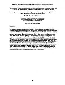
Figure 2: Mean accuracy and two standard deviations for 100 − 1600 hidden node ANNs on the 4,000-utterance ASR training set.
4.3
Obtaining the Oracles
For each training set for both ASR and OCR, ANNs of an increasing number of hidden nodes are trained and tested on the corresponding validation set. The size of the oracle ANN is chosen as the ANN with the highest average and least varying accuracy on the validation set (averaged over five different random initial weight settings). The oracle selection process is repeated for each training set, resulting in an oracle chosen for each of the four training set sizes. As an example, figure 2 shows mean accuracy and standard deviation for a given number of hidden nodes on a validation set for ANNs trained on the 4,000-utterance ASR training set. The ideal oracle ANN size in this case has 800 hidden nodes since it has the highest mean and lowest standard deviation. The same method is used to choose four oracles for ASR and four for OCR, one for each training set size. The same decaying learning rate is used to train every ANN (including the OTNs) and starts at 0.025, decaying according to
.025 p 1+ 5N
where p is the total number of patterns seen so far and N is the number of
patterns in the training set. This has the effect of decaying the learning rate by 10,
1 4
1 2
after five epochs,
1 3
after
after 15, etc. The initial learning rate and its rate of decay are chosen for their favorable performance
in our past experiments. 9
4.4
Labeling the Data Set and Training the OTNs
The four ASR oracles from section 4.3 create four oracle-labeled training sets using the entire 15, 000+ utterance (2.7 million phoneme) set whereas the four OCR oracles create four training sets using the 400,000 character training set, as described in section 3.2. The training sets are then used to train ANNs of sizes beginning with the first major break in accuracy, including 100, 50 and 20 hidden node ANNs for ASR and starting at either 512 or 256 hidden nodes for OCR and decreasing by halves until 32 hidden nodes.
4.5
Performance Criteria
For every training set size in section 4.2, and for every OTN size, five separate OTNs are trained using the training sets described in section 4.4, each with different, random initial weights. Even though there are only five experiments per OTN size on each training set, for ASR there are a total of 20 experiments for each of the three sizes across the four training sets and 15 experiments for each of the four training sets across the three sizes (for a total of 20 · 3 or 15 · 4 = 60 experiments). For OCR, this yields 10-20 experiments for each of the four OTN sizes and 20-25 experiments per training set size for at total of 90 experiments. After every oracle learning epoch, recognition accuracies are gathered using a hold-out set. The ANN most accurate on the hold-out set is then tested on the test set. The five test set results from the five OTNs performing best on the hold-out set are then averaged for the reported performance.
5 5.1
Results and Analysis Results
Table 1 summarizes the results of oracle learning. To explain how the table reads, consider the first row. The set size column has ASR and 150 meaning this is part of the ASR experiment and this row’s results were obtained using the 150 utterance training set. The OTN size column says 20 meaning this row is comparing 20 hidden node OTNs to 20 hidden node standard ANNs. The % Dec. Error column reads 36.01 meaning that using oracle learning resulted in a 36.01% decrease in error over standard training for 20 hidden node ANNs when using the 150 utterance training set. Decrease in error is calculated as:
1−
ErrorOT N ErrorStandard
(4)
The % Dec. error for OTN Size column gives 21.47 meaning averaged over the four training set sizes, oracle learning results in a 21.47% decrease in error over standard training for ANNs with 20 hidden nodes. This 10
Set OTN % Dec. Error % Avg Dec. error Average Similarity Size Size vs. Standard for OTN Size Similarity for OTN Size 20 50 100 Avg 20 500 50 100 Avg 20 1,000 50 100 Avg 20 4,000 50 100 Avg Avg
ASR 150
36.01 22.96 9.61 22.86 34.92 26.77 20.00 27.23 2.54 15.09 -5.29 4.11 12.42 0.95 5.94 6.44 15.16
21.47 16.44 7.56 21.47 16.44 7.56 21.47 16.44 7.56 21.47 16.44 7.56
0.9934 0.9981 0.9998 0.9971 0.9937 0.9994 1.0001 0.9977 0.9895 0.9977 0.9989 0.9953 0.9900 0.9967 0.9989 0.9953 0.9964
0.9916 0.9980 0.9994 0.9916 0.9980 0.9994 0.9916 0.9980 0.9994 0.9916 0.9980 0.9994
Set OTN % Dec. Error % Avg Dec. error Average Similarity Size Size vs. Standard for OTN Size Similarity for OTN Size 32 64 128 256 Avg 32 12.5% 64 128 256 512 Avg 32 25% 64 128 256 512 Avg 32 100% 64 128 256 Avg Avg OCR 5%
29.71 24.64 12.21 4.46 17.75 23.09 24.16 15.61 4.98 2.18 14.00 14.93 18.46 13.06 5.59 2.30 10.87 1.91 3.43 3.31 1.14 6.44 11.40
17.41 17.67 11.05 4.04 17.41 17.67 11.05 4.04 2.24 17.41 17.67 11.05 4.04 2.24 17.41 17.67 11.05 4.04
0.9773 0.9931 0.9977 0.9994 0.9919 0.9704 0.9906 0.9970 0.9992 0.9999 0.9914 0.9674 0.9883 0.9962 0.9993 1.0000 0.9902 0.9600 0.9836 0.9939 0.9977 0.9953 0.9895
0.9688 0.9889 0.9962 0.9989 0.9688 0.9889 0.9962 0.9989 0.9999 0.9688 0.9889 0.9962 0.9989 0.9999 0.9688 0.9889 0.9962 0.9989
Table 1: Combined ASR and OCR Results showing % decrease in error compared to standard training and oracle similarity.
11
number is repeated for each training set size for convenience in reading the table. The similarity column reads 0.9934 meaning that 20 hidden node OTNs retain 99.34% of their oracle’s accuracy for the 150 utterance case. Similarity is calculated as: Similarity =
AccuracyOT N AccuracyOracle
(5)
The average similarity for OTN size column reads 0.9916 meaning that averaged over the four training set sizes, 20 hidden node networks retain 99.16% of their oracles’ accuracy. The average decrease in error using oracle learning instead of standard methods is 15.16% averaged over the 60 experiments for ASR and 11.40% averaged over the 90 experiments for OCR. OTNs retain 99.64% of their oracles’ accuracy averaged across the 60 experiments for ASR and 98.95% of their oracles’ accuracy averaged across the 90 experiments for OCR. The results give evidence that as the amount of available labeled data decreases without a change in the amount of oracle-labeled data, oracle learning yields more and more improvement over standard training. This is probably due to the OTNs always having the same large amount of data to train on. They experience far more data points, and even though they are labeled by an oracle instead of by hand, the quality of the labeling is sufficient to exceed the accuracy attainable through training on only the hand labeled data.
5.2
Analysis
The results above provide evidence that oracle learning can be beneficial when applied to either ASR or OCR. With only one exception, the OTNs have less error than their standard trained counterparts. Oracle learning’s performance improves with respect to standard training if either the amount of labeled data or OTN size decreases. Therefore, for a given ASR application with only a small amount of labeled data, or given a case where an ANN of 50 hidden nodes or smaller is required for ASR or an ANN of 128 hidden nodes or less is required for OCR, oracle learning is particularly appropriate. The ASR 20 hidden node OTNs are an order of magnitude smaller than their oracles and are able to maintain 99.16% of their oracles’ accuracy averaged over the training set sizes with 21.47% less error than standard training. The 32 hidden node OTNs are two orders of magnitude smaller than their oracles but maintain 96.74% of their oracles’ accuracy with 17.41% less error than standard training. On average, oracle learning results in a 15.16% decrease in error for ASR and an 11.40% decrease in error for OCR compared to standard methods. Oracle learning also allows the smaller ANNs to retain 99.64% of their oracles’ accuracy on average for ASR and 98.95% or their oracles’ accuracy on average for OCR. Oracle learning’s positive performance is mostly likely do to there being enough oracle-labeled data points for the OTNs to effectively approximate their oracles. Since the larger, standard-trained oracles are always 12
better than the smaller, standard-trained ANNs, OTNs that behave like their oracles are more accurate than their standard-trained equivalents. Another reason for oracle learning’s performance may be that since the OTNs train to output targets between 0 and 1 instead of exactly 0 and 1, oracle learning presents a function that is easier for backpropagation to learn. Caruana [4, 5, 6] proved that for any classification function f (x), there may exist a function g(x) that represents the same solution, but is easier for backpropagation to learn. If this is the case for oracle learning, future work may result in a novel algorithm that produces easier, but equivalent functions for backpropagation to learn. However, future work will first focus on determining how varying the amount of available unlabeled instead of labeled data affects the performance of oracle learning.
5.3
Oracle Learning Compared to Pruning
As stated in section 2, both oracle learning and pruning can be used to produce a smaller ANN. The main difference is that with oracle learning, the smaller model is created initially and trained using the larger model, whereas with pruning, connections are removed from the larger model until the desired size is reached. Autoprune [11] is selected to compare pruning to oracle learning because it is shown to be more successful [18, 11] than the more popular methods in [20], and because it has a set pruning schedule. Lprune [18] adds an adaptive pruning schedule to autoprune, but it is designed to improve generalization accuracy and not to reduce model size explicitly. Lprune decides automatically how many connections to prune in terms of validation set accuracy, and may therefore never yield the desired number of connections. Lprune is meant to be used to improve overall accuracy and not, as is the case of oracle learning, to reduce the size of ANNs. To compare autoprune to oracle learning, first a 128 hidden node ANN is trained. Next, the 128 hidden node ANN is used as the oracle to train a 32 hidden node OTN (see section 3). Then, the larger ANN is pruned using autoprune’s schedule of first pruning 35% of the weights, then retraining until, in this case, a hold-out set suggests early stopping. The pruned ANN is then allowed to train once again until performance on a hold-out set stops increasing. After the pruned ANN is retrained, 10% of the remaining connections are pruned, followed by more retraining. This process continues pruning 10% at a time with results reported in two places. First, where the error of the pruned ANN is similar to that of the oracle trained ANN, and second, when the number of connections of the pruned ANN is similar to that of the oracle trained ANN. Table 2 shows the results of the experiment in order of highest accuracy. The top model is the original 128 hidden node ANN also used as the oracle ANN. The second line shows the auto-pruned ANN with an accuracy just above that of the OTN, the next model is the oracle trained ANN, the fourth compares the results of training a 32 hidden node network using standard methods, the fifth result shows the auto-pruned
13
Model Original ANN Auto-Pruned OTN STD Auto-Pruned Auto-Pruned Auto-Pruned
# Connections 18,944 8,079 4,736 4,736 7,271 4,771 4,294
Relative Size 4.00 1.71 1.00 1.00 1.54 1.01 0.91
Epochs 33 1634 198 256 2201 3774 4188
Accuracy 0.9656 0.9415 0.9338 0.9266 0.9199 0.6113 0.4966
Table 2: Oracle learning compared to autoprune ANN with an accuracy just below that of the OTN, and the bottom two results show the auto-pruned ANNs with a similar number of connections to the OTN. Notice that the pruned ANNs need more connections (1.54 to 1.71 times more) to obtain similar results to the OTN. Notice also that when allowed to prune to the same number of connections as the OTN, the auto-pruned ANNs have significantly lower accuracy. The results show pruning is not as effective as oracle learning when reducing an initial model to a specified size. In addition, the pruned ANNs required 10-20 times more training epochs. This suggests pruning is also less efficient than oracle learning.
5.4
Bestnets
As mentioned in section 1, another interesting area where we have succesfully applied oracle learning is approximating a set of ANNs that are “experts” over specific parts of a given function’s domain. The oracle learning solution we propose, namely bestnets, uses the set of “experts” as oracles to train a single ANN to approximate their performance. The application in which we have succesfully applied the bestnets method is to improve accuracy when training on data with varying levels of noise. A common solution to learning in a noisy environment is to train a single classifier on a mixed data set of both clean and noisy data. Often, the resulting classifier performs worse on clean data than a classifier trained only on clean data, and likewise for a classifier trained only on noisy data. It would be preferable to use the two domain specific classifiers instead, but this requires knowing if a given sample is clean or noisy—an often difficult problem to solve. Here, oracle learning can be used to approximate the two domain specific classifiers with a single OTN. The classifier trained only on noisy data and the classifier trained only on clean data can be used together as an oracle to label those parts of the training set that correspond to each model’s “expertise.” Initial results from McNemar tests [9] are shown in table 3. The ANN1 and ANN2 columns give the type of data used to train the models being compared. The data set column shows the type of data used to compare the two ANNs. The difference column gives the accuracy of ANN1 minus the accuracy of ANN2.
14
ANN1 Clean Data Oracle Noisy Data Oracle Bestnets Clean Data Oracle Noisy Data Oracle
ANN2 Mixed Data Mixed Data Mixed Data Bestnets Bestnets
Data set Clean Noisy Mixed Clean Noisy
Difference 0.0307 0.0092 0.0056 0.0298 -0.0011
p-value < 0.0001 < 0.0001 < 0.0001 < 0.0001 0.1607
Table 3: Results comparing the bestnets method to training directly on mixed data. The p-value column gives the p-value (lower is better) resulting from a McNemar test [9] for statistical difference between ANN1 and ANN2. A p-value of less than 0.0001 means that a difference as extreme or more than the difference between the two ANNs compared would be seen randomly less than 1 out of 1000 repeats of the experiment. In other words, the test is more than 99% confident that ANN1 is better than ANN2. Notice in the first two rows that the ANN trained on mixed data is significantly worse than the “expert” ANNs trained on their specific domains. This suggests there is room for improvement by using the bestnets method. The third row in the table shows that the bestnets ANN is significantly better than the ANN trained on mixed data when compared using both the noisy and clean data. It is expected that the bestnets ANN will miss one less in every 250 characters than the mixed data trained-ANN. The bestnets ANN is not significantly different than the ANN trained only on noisy data, yielding another improvement over directly training on the mixed data set. The bestnets method improves over training on the mixed data and retains the performance of the noise specific ANN. Future work will focus on increasing the improvement in accuracy of the bestnets method over standard training, especially on the clean data.
6
Conclusion and Future Work
6.1
Conclusion
On automatic spoken digit recognition oracle learning decreases the average error by 15.16% over standard training methods while still maintaining, on average, 99.64% of the oracles’ accuracy. For optical character recognition, oracle learning results in a 11.40% decrease in error over standard methods, maintaining 98.95% of the oracles’ accuracy, on average. The results also suggest oracle learning works best under the following conditions: 1. The size of the OTNs is small. 2. The amount of available hand-labeled data is small.
15
6.2
Future Work
One area of future work will investigate the effect of varying the amount of available unlabeled instead of labeled data. Another will determine if oracle learning presents a function that is easier to learn for backpropagation than the commonly used 0-1 encoding. If oracle learning does create an easier function, future research may lead to a novel algorithm that produces an equivalent, but easier function for back-propagation to learn. In addition, if oracle learning produces an easier function, it will outperform standard training on any data set, regardless of the availability of unlabeled data. A third area of future work will focus on increasing the bestnets method’s gains over direct training in a environment with varying levels of noise.
References [1] Kristin P. Bennett and Ayhan Demiriz. Exploiting unlabeled data in ensemble methods. [2] Avrim Blum and Tom Mitchell. Combining labeled and unlabeled data with co-training. In COLT: Proceedings of the Workshop on Computational Learning Theory, Morgan Kaufmann Publishers, 1998. [3] L. Breiman. Bagging predictors. Machine Learning., 24(2):123–140, 1996. [4] Rich Caruana. Algorithms and applications for multitask learning. In Proceedings of the Thirteenth International Conference on Machine Learning, pages 87–95, Bari, Italy, 1996. [5] Rich Caruana. Multitask Learning. PhD thesis, School of Computer Science, Carnegie Mellon University, Pittsburg, PA, 1997. [6] Rich Caruana, Shumeet Baluja, and Tom Mitchell. Using the future to “sort out” the present: Rankprop and multitask learning for medical risk evaluation. In David S. Touretzky, Michael C. Mozer, and Michael E. Hasselmo, editors, Advances in Neural Information Processing Systems, volume 8, pages 959–965, Cambridge, MA, 1996. The MIT Press. [7] Mark Craven and Jude W. Shavlik. Learning symbolic rules using artificial neural networks. In Paul E. Utgoff, editor, Proceedings of the Tenth International Conference on Machine Learning, pages 73–80, San Mateo, CA, 1993. Morgan Kaufmann. [8] Mark W. Craven and Jude W. Shavlik. Extracting tree-structured representations of trained networks. In David S. Touretzky, Michael C. Mozer, and Michael E. Hasselmo, editors, Advances in Neural Information Processing Systems, volume 8, pages 24–30, Cambridge, MA, 1996. The MIT Press.
16
[9] Thomas G. Dietterich. Approximate statistical test for comparing supervised classification learning algorithms. Neural Computation, 10(7):1895–1923, 1998. [10] Pedro Domingos. Knowledge acquisition from examples via multiple models. In Proceedings of the Fourteenth International Conference on Machine Learning, pages 98–106, San Francisco, 1997. Morgan Kaufmann. [11] William Finnoff, Ferdinand Hergert, and Hans Georg Zimmerman. Improving model selection by nonconvergent methods. Neural Networks, 6:771–783, 1993. [12] Sally Goldman and Yan Zhou. Enhancing supervised learning with unlabeled data. In Proc. 17th International Conf. on Machine Learning, pages 327–334. Morgan Kaufmann, San Francisco, CA, 2000. [13] Y. LeCun, B. Boser, J. S. Denker, D. Henderson, R. E. Howard, W. Hubbard, and L. D. Jackel. Handwritten digit recognition with a back-propagation network. In David Touretzky, editor, Advances in Neural Information Processing Systems II (Denver 1989), pages 396–404, San Mateo, CA, 1990. Morgan Kaufman. [14] Y. LeCun, J. Denker, S. Solla, R. E. Howard, and L. D. Jackel. Optimal brain damage. In D. S. Touretzky, editor, Advances in Neural Information Processing Systems II, San Mateo, CA, 1990. Morgan Kauffman. [15] G. R. Leonard and G. Doddington. Tidigits speech corpus, 1993. [16] Kamal Nigam and Rayid Ghani. Analyzing the effectiveness and applicability of co-training. In CIKM, pages 86–93, 2000. [17] Kamal Nigam, Andrew K. McCallum, Sebastian Thrun, and Tom M. Mitchell. Text classification from labeled and unlabeled documents using EM. Machine Learning, 39(2/3):103–134, 2000. [18] Lutz Prechelt. Adaptive parameter pruning in neural networks. Technical Report TR-95-009, International Computer Science Institute, Berkeley, CA, 1995. [19] J.R. Quinlan. C4.5: Programs for Machine Learning. Morgan Kaufmann, San Mateo, CA, 1993. [20] R. Reed. Pruning algorithms—a survey. IEEE Transactions on Neural Networks, 4(5):740–747, September 1993. [21] Alex Waibel, S. Hidefumi, and K. Shikano. Consonant recognition by modular construction of large phonemic time-delay neural networks. In Proceedings of the 6th IEEE International Conference on Acoustics, Speech, and Signal Processing., volume 1, pages 112–115, Glasgow, Scotland, 1989. 17
[22] Xinchuan Zeng and Tony Martinez. Using a neural networks to approximate an ensemble of classifiers. Neural Processing Letters., 12(3):225–237, 2000.
18