Artificial Neural Networks for Risk Decision Support in ... - Springer Link

Environmental Modeling and Assessment 9: 189–199, 2004.  2004 Kluwer Academic Publishers. Printed in the Netherlands.

Artificial neural networks for risk decision support in natural hazards: A case study of assessing the probability of house survival from bushfires Keping Chen a , Carol Jacobson b and Russell Blong a a Risk Frontiers – Natural Hazards Research Centre, Macquarie University, Sydney, NSW 2109, Australia b Department of Physical Geography, Macquarie University, Sydney, NSW 2109, Australia

Risk decision-making in natural hazards encompasses a plethora of environmental, socio-economic and management-related factors, and benefits greatly from exploring possible patterns and relations among these multivariate factors. Artificial neural networks, capable of general pattern classifications, are potentially well suited for risk decision support in natural hazards. This paper reports an example that assesses the risk patterns or probabilities of house survival from bushfires using artificial neural networks, with a simulation data set based on the empirical study by Wilson and Ferguson (Predicting the probability of house survival during bushfires, Journal of Environmental Management 23 (1986) 259–270). The aim of this study was to re-model and predict the relationship between risk patterns of house survival and a series of independent variables. Various configurations for input and output variables were tested using neural networks. An approach for converting linguistic terms into crisp numbers was used to incorporate linguistic variables into the quantitative neural network analysis. After a series of tests, results show that neural networks are capable of predicting risk patterns under all tested configurations of input and output variables, with a great deal of flexibility. Risk-based mathematical functions, be they linear or non-linear, can be re-modelled using neural networks. Finally, the paper concludes that the artificial neural networks serve as a promising risk decision support tool in natural hazards. Keywords: artificial neutral networks, natural hazards, risk decision-making, bushfire, linguistic terms

1. Introduction Risk decision-making in natural hazards is a multidimensional and multi-disciplinary activity embracing physical environmental, socio-economic and managementrelated factors at different spatial and temporal scales. Effective coupling of these multiple factors is a key to risk decision-making tasks (e.g., evaluation, prioritisation, selection). Conventional methods of multi-criteria evaluation (e.g., weighted linear combination, compromise programming) can be used to support such tasks and provide a mechanism to assemble, weight, synthesise and analyse a wide range of data layers [1]. However, the conventional methods are sometimes less favoured because: (1) determining relative weights between criteria is a subjective process and often requires a priori knowledge; (2) simple aggregation methods may not be adequate for representing relations between criteria that are essentially non-linear; and (3) handling different data types is difficult (e.g., [1,4,7]). These and other concerns of the conventional multi-criteria evaluation methods provide impetus for seeking alternative risk decision support techniques that are capable of effectively integrating various data layers, evaluating complex rules and recognising non-linear relationships across criteria. Recent developments in broader decision support research show that modern artificial intelligence methods, including artificial neural networks (ANN), fuzzy sets theory and genetic algorithms, have potential advantages in dealing with the above limitations [4,16]. For example, ANN are most likely to be superior to other statistical methods

in situations where (1) relations between data exhibit nonlinearity; (2) patterns important to the decision task are subtle or deeply hidden; and (3) the input data are fuzzy, involving human opinions and ill-defined categories, or subject to possible error and uncertainty [5]. During the past few decades, ANN have been used for decision support in various geographical and environmental problems [6,10,12], including land use planning [19], land cover classification [3], forest resource management [4], land use suitability assessment [16], mapping environmental carrying capacity [9] and desertification assessment [15]. This paper applies ANN methodology for risk decision support in natural hazards. Prior to informed risk decisionmaking, one needs to understand and quantify complex patterns and relations between elements at risk (exposures) and hazard factors, e.g., relations between flooded building damage and water velocity and inundation depth, between infrastructure damage and earthquake ground motion, between house survival probability and bushfire intensity. Here, disparate data on hazard, exposure and vulnerability, which could be fuzzy, unquantifiable and incomplete, should be effectively dealt with. Hazard levels, for example, may be represented by linguistic terms (e.g., “low”, “medium”, “high”); to include them in an ANN analysis a conversion approach from linguistic terms to crisp values is necessary. To illustrate neural networks as a new approach for risk decision support, we present an example which assesses the probabilities of house survival during bushfires using various data on the hazard and characteristics of the houses.

190

K. Chen et al. / Artificial neural networks for risk decision support in natural hazards

2. Artificial neural networks methodology A fundamental aspect of ANN is the use of processing elements that are analogous models of neurons in the brain. These processing elements are connected together in a structured and adaptive manner in which the links can be dynamically modified through weights. The network can be trained to recognise patterns in input data and then can not only recognise such patterns when they occur again, but also identify similar patterns. Such special features of learning and generalisation make ANN distinct from conventional methods [14]. Among various neural network paradigms, the most commonly used are supervised feedforward neural networks, trained by error backpropagation algorithms. They are referred to as backpropagation neural networks.

Supervised learning can be achieved by minimising the errors between the calculated and the desired output values through error backpropagation computation and modifying the connection weights. When the error converges to a userspecified threshold value, or the prescribed number of training cycles that produces a reasonably small error is reached, it is considered that the network has “learned” the training pattern and is ready for testing. Detailed mathematical descriptions of ANN and error backpropagation algorithms and discussion aspects of network improvements can be found in Hagan et al. [5]. Major steps of an ANN application, from the configuration of a network typology to training and testing the network to assessing network performance, are presented in the case study. 2.2. Conversion of linguistic terms to crisp values

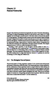
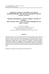
2.1. Backpropagation neural networks Neural networks typically consist of an input layer, an output layer, and at least one hidden layer (figure 1). The input layer is composed of one or more processing elements that present raw data (usually after standardisation) to the network. Input data are processed from input layer to the hidden layer, and then to the output layer containing patterns to be learned. Processing elements in the neighbouring layers are connected by weights. All processing elements, except those in the input layer, perform two functions: collecting the inputs of the processing elements in the previous layer and through activation functions generating an output (figure 2). Mathematically, an input (neti ) of a processing element i can be calculated from the outputs oj of processing elements in the previous layer, the weights wij of the connections and bias bi , as shown in equation (1). Then, an activation transfer function f , usually with a sigmoidal form, is followed. wij oj + bi . (1) neti = j

Figure 1. An example of a neural network: 4 variables in an input layer, 2 variables in a hidden layer, and 3 variables in an output layer.

Linguistic terms in an ANN-based risk decision support study can be processed with fuzzy sets theory. From a methodological perspective, artificial neural networks and fuzzy sets theory are complimentary as fuzzy sets can be used to enhance the networks by (1) preprocessing of input data to improve the learning mechanisms of the networks; (2) incorporating fuzzy logic-oriented IF–THEN rules in fine tuning the inputs and outputs of the networks; and (3) making linguistic interpretation of the results produced by the networks (e.g., [8]). In this paper, the preprocessing of linguistic terms for an ANN analysis is used. Chen and Hwang [2] proposed a numerical approximation system to systematically convert linguistic terms to corresponding fuzzy sets and then to crisp values. The system was based on previous extensive empirical studies on the use of linguistic terms, and is composed of eight conversion scales and 11 verbal terms in a universe U = {excellent, very high, high to very high, high, fairly high, medium, fairly low, low, low to very low, very low, none}. This universe can be accommodated to fit individual criteria in a risk decision-making framework. For example, if a hazardous event is one of the criteria, the possible universe could be {extremely dangerous, very dangerous, . . . , moderate, . . . , very safe, extremely safe}. The fuzzy sets corresponding to these verbal terms can be estimated using one of the eight conversion scales. The first seven scales with calculated sets

Figure 2. A neuron as a processing element.


191

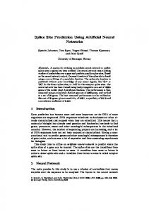
Figure 3. Seven scales for converting linguistic terms to fuzzy sets and crisp values according to Chen and Hwang [2]. Calculated values are listed with corresponding conversion scales.

of crisp values are shown in figure 3. The calculation of crisp values from fuzzy sets is described in Chen and Hwang ([2], pp. 474–476). The 8th scale containing 11 verbal terms is omitted because it is rarely used, being too complex for

many risk decision-making tasks. Easy-to-use conversion scales can be intuitively understood by a wide range of practitioners, so they are of potential value for wider applications.

192


• Presence of plants taller than 5 m high within 2–40 m of the house: present (x9 = 1), absence (x9 = 0).

3. An example of assessing the probability of house survival In Australia bushfires are widespread especially in prolonged hot and dry summer seasons. Bushfires constantly threaten and even destroy houses constructed in the fireprone bushland-urban interface. For example, the February 1983 “Ash Wednesday” bushfires that occurred in Victoria and South Australia and the January 1994 Sydney bushfires destroyed about 2500 and 200 houses, respectively [13]. The probability of house survival from bushfires is affected by a wide array of factors, including proximity to bushland, building design and construction (e.g., roof and wall materials), and surrounding environments (e.g., vegetation amount and density). Empirical studies on the estimation of house survival using conventional statistical analysis of post-fire survey data have been reported by Wilson and Ferguson [18], and Ramsay et al. [13]. This section investigates the use of ANN, as opposed to the conventional statistical methods, for classifying patterns of house survival with simulated data based on the study of Wilson and Ferguson [18]. Wilson and Ferguson [18] applied logistic regression to model the probability of house survival with detailed observations of 450 houses affected by the “Ash Wednesday” bushfires at Mount Macedon, Victoria. In the regression, the dependent variable (the probability of house survival) was a binary variable: survived (if the damage was slight) or destroyed (if the damage was extensive). The independent or explanatory variables (i.e., x1 , x2 , . . . , x9 ) were factors affecting house survival. The estimated probability of house survival (p) was a function of a composite hazards score (H ). exp(6.3 − H ) p= 1 + exp(6.3 − H )

(2)

where H = 2.2 × x1 + 0.8 × x2 + 2.4 × x3 + 1.4 × x4 + 5.2 × x5 + 3.6 × x6 + 2.3 × x7 + 1.1 × x8 + 0.6 × x9 . The coefficient of each factor indicates its relative importance. All factors used a binary format, as detailed below: • Attendance by residents: unattended (x1 = 1), attended (x1 = 0). • Presence of flammable objects: present (x2 = 1), absence (x2 = 0). • Roof material and pitch: Roof is wooden (x3 = 1), not (x3 = 0). Roof (not wooden, not tiled) has a pitch > 10◦ (x4 = 1), not (x4 = 0). • Fire intensity (kW m−1 ): >10 000 (x5 = 1), not (x5 = 0). [1500–10 000] (x6 = 1), not (x6 = 0). [500–1499] (x7 = 1), not (x7 = 0). • Wall material: wood, fibro or other non-brick material (x8 = 1), brick (including brick-veneer), stone or cement (x8 = 0).

Of the above factors, only the fire intensity cannot be observed directly and should be estimated first. Their estimation suggested that about 10% of all 450 houses were exposed to a fire of intensity [10 000–60 000 kW m−1 ], about 50% to a fire of intensity [1500–10 000 kW m−1 ] and the remaining 40% to a less intense fire [17,18]. Given the estimated fire intensity (x5 or x6 or x7 ), along with other factors (x1 , x2 , x3 , x4 , x8 , x9 ), the probability of individual house survival could be predicted (figure 4). 3.1. Generating a simulation data set Since the original post-fire survey data set used by Wilson and Ferguson [18] is lost and no comparable data are available, a set of simulation data was produced based on the equation (2). First, a total of 200 sample dwellings were simulated by randomly generating values for the above nine variables. The distribution of fire intensity (x5 or x6 or x7 ) was based on the reported percentage of houses experiencing different fire intensities in the original study [18]. Values of x1 , x2 , . . . , x9 represent attributes of the 200 houses; p is the calculated probability using the above equation (figure 4). Because x1 , x2 , . . . , x9 were treated as independent variables, and p (the dependent variable) was calculated using the known equation, there is no reason to suspect their validity. 3.2. Selecting input and output variables For the neural networks, the first step is to specify a series of independent variables as network inputs and a dependent variable as a network output. Careful treatments of the input and output variables are needed in neural network applications, such as scaling the distributions of variables (e.g., linear transformation) and dealing with outliers and missing data [11]. Often, a binary format is used for coding the network inputs and outputs [16]. When the input and output of the network are not hard physical measurements, but include linguistic terms, subjective responses or memberships in illdefined categories, these data can be quantified by using the conversion scales in figure 3 or a surrogate. To re-model and predict the relationship between probabilities of house survival and independent variables, the nine input variables (x1 , x2 , x3 , x4 , x8 , x9 , fire intensity x5 or x6 or x7 ) and an output variable (p) were used. Two configurations of the input and output variables for the neural networks were examined: (1) the form of output variable as a continuous value remained the same, while different forms of the input variables were considered; and (2) the form of the input variables were unchanged, while different discrete forms of the output variable were considered. Using the various configurations of input and output variables, neural networks were constructed to identify risk patterns in either continuous probabilities form or discrete risk levels.


193

Figure 4. Example data and the estimated probability curve for house survival in relation to hazard factors according to Wilson and Ferguson [18].

In the first configuration, the six independent variables (x1 , x2 , x3 , x4 , x8 , x9 ) used an “as is” binary format and the fire intensity was expressed as the following two forms: Mode A – binary variables; and Mode B – linguistic terms. In Mode A, the fire intensity was expressed as three binary variables (x5 , x6 , x7 ). Therefore, in this mode all nine input variables and the output variable were the same form as the variables used in [18]. Under this scenario, neural networks were simply used to re-model the relationship between the independent variables and the dependent variable that was derived using logistic regression by Wilson and Ferguson [18]. In Mode B, the fire intensity was expressed as linguistic terms. According to Wilson and Ferguson [18], in order to derive the probability of house survival, a quantitative estimation of fire intensity must be first performed. However, in some cases, detailed quantitative estimation may be difficult while verbal quantification may be easy and efficient based on local expertise. Quantification could be in linguistic terms such as the ones used in figure 3. For example, based on figure 3(e), various linguistic terms corresponding with different levels of fire intensities [18] can be used. “very high”: [10 000–60 000] kW m−1 ; “high”: [1500–10 000] kW m−1 ; “fairly low”: [500–1500] kW m−1 ; and “very low”: less than 500 kW m−1 . These linguistic terms can be easily converted into crisp numbers which are then used as inputs to the neural networks, instead of using the binary format of variables (x5 or x6 or x7 ). The four linguistic terms “very high”, “high”,

“fairly low” and “very low” were expressed as crisp numbers of 0.9167, 0.75, 0.4167 and 0.0833, respectively (figure 3(e)). In this mode, seven input variables were used: fire intensity expressed as only one variable and the other six variables (x1 , x2 , x3 , x4 , x8 , x9 ). Although the linguistic terms in this example were based on the four levels of fire intensity prescribed by Wilson and Ferguson [18], the main aim here was to demonstrate that linguistic terms can be incorporated into a quantitative analysis in a straightforward manner and to determine whether the neural networks can reveal the expected relationship when another value form of the input variable is applied. Unlike the first configuration, which used the probability of house survival as a continuous variable, the second configuration used discrete output values to represent risk patterns of house survival. A binary risk pattern – survived (1) or destroyed (0) was first considered. The specification of binary risk patterns was based on the calculated probability of house survival. However, there was no clear division or prior knowledge to define this. It was assumed that houses that survived had a high probability of house survival, while destroyed houses corresponded to a low probability of house survival. Therefore, a new output variable that groups survived and destroyed houses based on probability ranges was examined. For example, the probability of 0.4 was first used as a division to group survived (0.4 probability < 1) and destroyed (0 < probability < 0.4) houses, giving a binary data set as the output. Three more experiments using different probability divisions (i.e., 0.5, 0.6 and 0.7) were also tested.

194


To further test the pattern classification capabilities of neural networks, this study considered another set of discrete risk patterns based on the calculated probability. Five discrete levels of house survival were defined as follows: Level 5 (“very high”) 0.8 p < 1.0; Level 4 (“high”) 0.6 p < 0.8; Level 3 (“medium”) 0.4 p < 0.6; Level 2 (“low”) 0.2 p < 0.4; Level 1 (“very low”) 0.0 p < 0.2. 3.3. Preparing training and testing data The data set containing the input and output variables is divided into two files: (1) training data subset; and (2) testing data subset. It is important to ensure that the training samples given to the network cover the range of possibilities and are representative of the frequency of occurrences of the variables [11]. Training data may be defined by observations, experimental results and expert knowledge. The testing data are used to check the ability of the supposedly trained networks for generalisation, and to assess the ability of the networks for estimating the proposed output correctly. In this study, 150 simulated samples in a random order formed the training data file while the remaining 50 simulated samples in a random order were used for network testing. 3.4. Network design and configuration The number of processing elements in the input layer is generally decided by the number of independent variables involved, and the number of processing elements in the output layer is determined by the number of dependent variables. In most cases, a three-layer network is sufficient [11]. Therefore, networks used for this study consisted of the input layer of nine processing elements (except for the networks used in the Mode B, where seven input processing elements were used), one hidden layer, and the output layer of one processing element representing either the probability of house survival in the first configuration or the discrete risk levels in the second configuration. A program called NNMODEL, which automatically generates the optimum number of processing elements in the hidden layer, was used in the analysis. 3.5. Network training The networks used in the first configuration were trained using 5000 training cycles, with the summed squared errors of 0.00003 in Mode A and 0.00036 in Mode B. All trained networks had four processing elements in the hidden layer. Figure 5 displays the results of the neural networks after training for the first configuration; random samples are ranked according to their probabilities of house survival to clearly show the difference between the outputs of the networks and the original sample probabilities.

Figure 5. Results after training the neural networks for the first configuration. (a) Mode A, and (b) Mode B. The x-axis shows the 150 training samples, and the y-axis the probability of house survival.

In Mode A, the probabilities of house survival from the trained network are virtually matched with the sample risk patterns. R 2 between the trained data and sample data is 0.999. This suggests that the network can learn the relationship between the input and output data precisely. The output was originally calculated by an additive hazard score and a non-linear curve [18], and the result here indicates this relationship can be reconstructed with an ANN network. From a theoretical perspective, it is known that the neural networks can be used to approximate linear or non-linear functions [5]. This versatility implies that the relationship between disparate factors expressed in a traditional mathematical equation can also be modelled using neural networks. In Mode B, the risk patterns after training are also almost matched with the sample probabilities. R 2 between the trained outputs and sample probabilities is 0.989. This demonstrates that linguistic terms after appropriate “soft digitising” can also be used with neural networks. For the second configuration, the results of four trained networks with binary risk patterns are shown in figure 6. Although samples input to the networks were mixed, they were grouped into either survived (1) or destroyed (0) houses for the purposes of clearer visualisation and interpretation (figure 6). When different probability divisions were used, the numbers of survived and destroyed houses varied (table 1). The four trained networks produced very impressive results of pattern recognition. For example, from figure 6(a), 55 of 75 samples for the survived houses and 59 of 75 samples for the destroyed houses were accurately trained (table 1), and the results of all other samples did not show wide deviations. For the five discrete risk levels, the network was trained for 5000 cycles and resulted in a summed square error of 0.00133. From figure 7(a), the outputs after training closely


195

Figure 7. Results from the neural networks for the second configuration using five discrete risk levels. (a) Trained results of 150 samples, and (b) Predicted results of 50 testing samples. The x-axis shows samples, and the y-axis risk patterns.

Figure 6. Results after training the neural networks for the second configuration. Different probability divisions of house survival were used to group survived (1) and destroyed (0) houses: (a) 0.4, (b) 0.5, (c) 0.6, and (d) 0.7. The x-axis shows the 150 training samples, and the y-axis risk patterns. Table 1 Results after training the networks for the second configuration: four probability divisions (i.e., 0.4, 0.5, 0.6, and 0.7) were used with 150 simulated training samples. Binary output with four probability divisions

No. of survived houses (1) Exactly trained for (1) No. of destroyed houses (0) Exactly trained for (0) Summed squared error

0.4

0.5

0.6

0.7

75 55 75 59 0.00087

64 44 86 74 0.00083

45 35 105 73 0.00104

21 13 129 115 0.00056

match with the sample patterns: all samples were trained with deviations less than one risk level. 3.6. Testing the networks After training has been completed, the testing stage is used to indicate the predictive power of the neural network modelling for risk pattern classification. The testing data set consisting of the 50 randomly ordered samples was applied

to the input layer of the trained networks and proceeded to the output layer. Then, outputs were compared with the sample probabilities of house survival. The results for the first configuration are shown in figure 8. It is evident that the predictive capability of the network is excellent. The R 2 between the predicted and sample patterns in Mode A and B are 0.989 and 0.968, respectively. Predicted risk patterns closely matched the sample probabilities except for one house. The large differences of that one sample are difficult to explain. One possible reason is that the number of samples used to train the network was not large enough to represent the input and output relationship from the limited training data. Results for Mode B confirm that the neural network was able to accurately predict house survival when only linguistic terms are available to describe fire intensity. The results of the network tests for the second configuration are shown in figure 9 and table 2. Comparing the binary sample and predicted risk patterns, the four trained networks were able to classify well. For example, with the probability division of 0.4, the 50 test samples were composed of 28 samples of survived houses and 22 samples of destroyed houses; 16 of 28 samples of survival and 17 of 22 of destruction were exactly predicted. Except for three samples where house survival was wrongly predicted, all other samples were predicted well with only a small amount of deviation (figure 9(a)). Similarly, with the other probability divisions only a small percentage of houses were incorrectly predicted. Finally, in the test of five discrete risk levels all were predicted well (figure 7(b)) with deviations less than one level,

196


Figure 8. Predicted results of the testing samples for the first configuration. (a) Mode A, and (b) Mode B. The x-axis shows the 50 testing samples, and the y-axis the probability of house survival. Table 2 Results of testing the networks for the second configuration: four probability divisions (i.e., 0.4, 0.5, 0.6, and 0.7) were used with 50 simulated testing samples. Binary output with four probability divisions

No. of survived house (1) Exactly predicted for (1) Wrongly predicted for (1)* No. of destroyed houses (0) Exactly predicted for (0) Wrongly predicted for (0)*

0.4

0.5

0.6

0.7

28 16 3 22 17 0

22 8 0 28 21 1

14 5 2 36 18 3

9 2 0 41 33 0

* If the deviation of 0.5 was used.

except for one sample of the risk level of 5 (“very high”) and two samples of the risk level of 3 (“moderate”). 3.7. Summary

Figure 9. Predicted results of the testing samples for the second configuration, using different probability divisions of house survival to group survived (1) and destroyed (0) houses: (a) 0.4, (b) 0.5, (c) 0.6, and (d) 0.7. The x-axis shows the 50 testing samples, and the y-axis risk patterns.

Using the simulation data set with various configurations of the input and output variables, neural networks were capable of re-modelling and predicting relationships between risk patterns of house survival (i.e., continuous risk probabilities and discrete risk levels) and independent variables reported by Wilson and Ferguson [18]. Encouraging results suggest that neural networks have advanced ability and flexibility of pattern recognition, and can supplement or even replace conventional approaches, which are based on the assumption of the additive nature of hazards and vulnerability factors. However, some aspects can be further explored. For example, in Mode B the four linguistic terms were exempli-


fied according to predefined levels of fire intensity; other thresholds for classifying the fire intensity can also be tested. In addition to the attributional analysis, if locations of individual houses were available, their spatial risk patterns can be mapped and spatial relations could be examined. Moreover, various neural network tests could be applied to samples with more input factors (e.g., aspect, slope, presence/absence of large unprotected windows or glass doors), detailed classes of risk patterns and even with some noisy and incomplete data. 4. Concluding remarks Since risk decision-making can benefit tremendously from the process of effective data mining and knowledge discovery, it is vital to apply new, versatile statistical approaches that can shed light on complex relations among disparate factors. In this regard, artificial neural networks with strong pattern classification capabilities offer a promising tool. Applications of modern artificial intelligence methods in hazard risk decision support are in their infancy, and this study serves as a call for drawing more attention to the potential utility of modern methodologies in risk managers’ decision-making tasks. The increasing availability of easy-to-use programs for various artificial intelligence methods now enables wider and in-depth real-world applications. Appendix

(1) A training data set consisting of 150 simulated samples. Fire x1 x2 x3 x4 x8 x9 H Probability 0.41 0.5 0.6 0.7 5-level intensity (p) risk pattern2 (kW m−1 ) 3100 4010 1230 789 4390 9600 3200 564 1200 340 789 3400 1049 5200 8900 8402 4507 982 2500 1400 187 380

1 0 0 0 0 0 1 0 1 1 0 0 1 0 0 0 1 1 1 1 0 0

1 0 1 1 0 1 0 1 1 0 1 0 1 0 1 1 1 1 1 0 1 1

1 1 0 0 1 0 0 0 1 0 1 0 1 0 0 0 1 0 0 0 1 1

1 1 1 1 0 0 0 1 0 1 1 0 0 1 0 1 0 0 0 1 1 1

0 1 1 1 1 0 0 0 0 1 1 1 0 1 1 1 0 0 0 0 1 1

1 11 1 9.1 0 5.6 0 5.6 0 7.1 1 5 0 5.8 0 4.5 1 8.3 0 4.7 0 8 0 4.7 0 7.7 0 6.1 0 5.5 1 7.5 1 9.6 1 5.9 0 6.6 0 5.9 0 5.7 0 5.7

0.009013 0.057324 0.668188 0.668188 0.310026 0.785835 0.622459 0.858149 0.119203 0.832018 0.154465 0.832018 0.197816 0.549834 0.689974 0.231475 0.035571 0.598688 0.425557 0.598688 0.645656 0.645656

0 0 1 1 0 1 1 1 0 1 0 1 0 1 1 0 0 1 1 1 1 1

0 0 1 1 0 1 1 1 0 1 0 1 0 1 1 0 0 1 0 1 1 1

0 0 1 1 0 1 1 1 0 1 0 1 0 0 1 0 0 0 0 0 1 1

0 0 0 0 0 1 0 1 0 1 0 1 0 0 0 0 0 0 0 0 0 0

1 1 4 4 2 4 4 5 1 5 1 5 1 3 4 2 1 3 3 3 4 4

197

Fire x1 x2 x3 x4 x8 x9 H Probability 0.41 0.5 0.6 0.7 5-level intensity (p) risk (kW m−1 ) pattern2 9300 28765 2989 4690 1450 750 2000 289 34001 13009 5120 562 567 2865 1090 2090 43098 909 1267 4900 57287 51888 542 2340 890 19780 698 6700 5600 1278 2300 4900 1989 3670 129 980 1966 4312 6200 674 1209 89 4500 8200 4300 1106 654 6722 230 890 8500 16000 3400 1760 4500 4300 19002 3965 455 2678 670

0 1 0 1 1 0 0 0 1 1 0 0 1 0 0 1 1 1 0 0 1 0 1 1 1 0 1 1 1 1 1 1 0 0 1 0 0 0 0 1 0 1 1 1 0 0 0 1 1 0 1 0 1 1 1 1 0 0 1 0 1

0 0 1 1 1 0 0 1 0 0 1 0 0 0 0 1 0 1 1 1 1 0 0 0 1 0 0 0 0 0 0 0 0 1 0 0 0 0 1 1 1 0 0 0 0 1 1 0 1 0 1 1 0 0 1 0 1 1 1 1 0

0 0 0 0 0 0 1 1 1 1 1 1 1 0 0 1 1 1 0 0 1 0 0 1 0 1 0 0 0 0 0 0 0 1 0 1 0 1 1 1 0 1 0 0 1 0 1 0 1 1 1 0 1 1 0 0 0 1 0 1 0

1 0 0 0 1 1 1 0 1 1 0 0 0 1 1 0 0 1 1 0 0 1 0 1 0 1 1 0 0 1 1 1 1 1 0 1 1 0 0 0 1 1 0 0 0 1 0 0 0 0 0 1 0 0 0 1 0 1 0 0 1

0 0 1 0 1 1 1 1 1 1 0 1 1 0 1 1 1 1 0 1 1 0 1 1 0 1 1 0 0 1 0 1 1 1 1 0 1 0 1 0 1 1 1 0 0 1 0 0 0 0 1 0 1 0 0 1 0 0 1 1 1

1 0 0 0 1 0 1 1 0 1 1 0 0 0 1 1 0 1 0 1 0 1 1 1 0 1 0 1 1 1 0 0 0 0 0 0 0 1 0 1 1 0 1 0 0 0 1 0 1 1 0 1 1 0 0 1 0 1 0 1 1

5.6 7.4 5.5 6.6 8.4 4.8 9.1 4.9 12.3 12.9 7.4 5.8 8 5 5.4 10.7 10.9 10.8 4.5 6.1 11.7 7.2 6.2 11.3 5.3 10.7 7 6.4 6.4 7.6 7.2 8.3 6.1 9.3 3.3 6.1 6.1 6.6 7.9 8.3 6.2 7.1 7.5 5.8 6 5.6 6.1 5.8 6 5.3 10.1 8 9.9 8.2 6.6 8.9 6 8.8 4.1 8.5 7.6

0.668188 0.24974 0.689974 0.425557 0.109097 0.817574 0.057324 0.802184 0.002473 0.001359 0.24974 0.622459 0.154465 0.785835 0.71095 0.012128 0.009952 0.010987 0.858149 0.549834 0.004496 0.28905 0.524979 0.006693 0.731059 0.012128 0.331812 0.475021 0.475021 0.214165 0.28905 0.119203 0.549834 0.047426 0.952574 0.549834 0.549834 0.425557 0.167982 0.119203 0.524979 0.310026 0.231475 0.622459 0.574443 0.668188 0.549834 0.622459 0.574443 0.731059 0.021881 0.154465 0.026597 0.130108 0.425557 0.069138 0.574443 0.075858 0.90025 0.09975 0.214165

1 0 1 1 0 1 0 1 0 0 0 1 0 1 1 0 0 0 1 1 0 0 1 0 1 0 0 1 1 0 0 0 1 0 1 1 1 1 0 0 1 0 0 1 1 1 1 1 1 1 0 0 0 0 1 0 1 0 1 0 0

1 0 1 0 0 1 0 1 0 0 0 1 0 1 1 0 0 0 1 1 0 0 1 0 1 0 0 0 0 0 0 0 1 0 1 1 1 0 0 0 1 0 0 1 1 1 1 1 1 1 0 0 0 0 0 0 1 0 1 0 0

1 0 1 0 0 1 0 1 0 0 0 1 0 1 1 0 0 0 1 0 0 0 0 0 1 0 0 0 0 0 0 0 0 0 1 0 0 0 0 0 0 0 0 1 0 1 0 1 0 1 0 0 0 0 0 0 0 0 1 0 0

0 0 0 0 0 1 0 1 0 0 0 0 0 1 1 0 0 0 1 0 0 0 0 0 1 0 0 0 0 0 0 0 0 0 1 0 0 0 0 0 0 0 0 0 0 0 0 0 0 1 0 0 0 0 0 0 0 0 1 0 0

4 2 4 3 1 5 1 5 1 1 2 4 1 4 4 1 1 1 5 3 1 2 3 1 4 1 2 3 3 2 2 1 3 1 5 3 3 3 1 1 3 2 2 4 3 4 3 4 3 4 1 1 1 1 3 1 3 1 5 1 2

198


Fire x1 x2 x3 x4 x8 x9 H Probability 0.41 0.5 0.6 0.7 5-level intensity (p) risk pattern2 (kW m−1 ) 690 419 3745 6078 4577 3200 1299 50 6766 4312 29455 7972 1400 5989 1090 2300 1789 762 1090 15000 1923 5609 4587 876 1345 1056 12065 330 4120 7620 609 6987 1456 4599 8120 1866 4390 21090 5286 1278 980 4210 632 19087 6783 1402 4500 7908 1700 875 9500 4809 3266 8360 1462 78 98 5600 8878 5612 980 7432 120 48622

0 0 0 0 0 1 0 0 1 0 0 0 0 1 0 1 0 0 0 1 1 0 0 0 0 0 1 0 0 1 0 1 0 1 1 1 0 0 0 1 1 1 1 0 1 1 1 1 0 1 0 0 0 0 1 0 0 1 0 0 1 0 0 0

1 0 0 1 1 0 1 1 1 1 1 1 1 0 1 1 0 1 1 0 0 0 0 1 0 0 1 0 1 0 1 1 0 1 1 1 0 1 1 0 0 0 0 0 0 1 1 0 1 0 1 1 0 1 1 1 1 1 1 1 0 1 1 1

0 1 1 1 0 0 1 1 1 0 0 1 1 0 1 1 1 1 0 1 0 0 0 1 1 1 1 1 0 1 1 0 0 1 0 1 1 1 1 1 1 1 0 0 0 1 0 0 0 0 0 0 1 1 0 1 0 0 0 0 0 0 0 1

1 1 0 1 0 0 0 0 0 1 0 0 0 1 0 0 0 1 1 0 0 0 0 1 0 1 0 1 1 1 1 1 0 1 0 1 1 0 1 1 0 0 0 1 0 0 1 0 1 0 1 1 0 0 1 1 1 1 1 0 0 1 1 0

1 1 0 0 1 1 0 0 1 0 0 0 0 0 1 0 1 1 1 1 1 1 0 0 1 0 0 0 0 0 1 0 1 0 1 1 0 0 1 1 1 1 0 0 1 1 1 0 1 1 0 0 1 1 1 0 1 0 0 1 1 1 1 1

1 1 0 0 0 0 0 1 0 0 1 0 0 0 0 0 1 0 0 1 1 1 0 1 0 0 1 0 0 0 1 0 1 0 0 1 0 0 1 1 1 0 1 0 1 0 1 0 0 1 0 1 1 1 0 1 1 0 1 0 1 0 0 0

6.2 5.5 6 8.2 5.5 6.9 5.5 3.8 10.1 5.8 6.6 6.8 5.5 7.2 6.6 9 7.7 8 5.6 11.5 7.5 5.3 3.6 7.5 5.8 6.1 11.2 3.8 5.8 9.6 8.6 8 4 10.4 7.7 12.1 7.4 8.4 9.9 10 8.6 9.3 5.1 6.6 7.5 8.8 9.7 5.8 6.9 6.2 5.8 6.4 7.7 8.5 7.8 5.2 3.9 8 6.4 5.5 6.2 6.9 3.3 9.5

0.524979 0.689974 0.574443 0.130108 0.689974 0.354344 0.689974 0.924142 0.021881 0.622459 0.425557 0.377541 0.689974 0.28905 0.425557 0.062973 0.197816 0.154465 0.668188 0.005486 0.231475 0.731059 0.937027 0.231475 0.622459 0.549834 0.007392 0.924142 0.622459 0.035571 0.091123 0.154465 0.908877 0.016302 0.197816 0.003018 0.24974 0.109097 0.026597 0.024127 0.091123 0.047426 0.768525 0.425557 0.231475 0.075858 0.032295 0.622459 0.354344 0.524979 0.622459 0.475021 0.197816 0.09975 0.182426 0.75026 0.916827 0.154465 0.475021 0.689974 0.524979 0.354344 0.952574 0.039166

1 1 1 0 1 0 1 1 0 1 1 0 1 0 1 0 0 0 1 0 0 1 1 0 1 1 0 1 1 0 0 0 1 0 0 0 0 0 0 0 0 0 1 1 0 0 0 1 0 1 1 1 0 0 0 1 1 0 1 1 1 0 1 0

1 1 1 0 1 0 1 1 0 1 0 0 1 0 0 0 0 0 1 0 0 1 1 0 1 1 0 1 1 0 0 0 1 0 0 0 0 0 0 0 0 0 1 0 0 0 0 1 0 1 1 0 0 0 0 1 1 0 0 1 1 0 1 0

0 1 0 0 1 0 1 1 0 1 0 0 1 0 0 0 0 0 1 0 0 1 1 0 1 0 0 1 1 0 0 0 1 0 0 0 0 0 0 0 0 0 1 0 0 0 0 1 0 0 1 0 0 0 0 1 1 0 0 1 0 0 1 0

0 0 0 0 0 0 0 1 0 0 0 0 0 0 0 0 0 0 0 0 0 1 1 0 0 0 0 1 0 0 0 0 1 0 0 0 0 0 0 0 0 0 1 0 0 0 0 0 0 0 0 0 0 0 0 1 1 0 0 0 0 0 1 0

3 4 3 1 4 2 4 5 1 4 3 2 4 2 3 1 1 1 4 1 2 4 5 2 4 3 1 5 4 1 1 1 5 1 1 1 2 1 1 1 1 1 4 3 2 1 1 4 2 3 4 3 1 1 1 4 5 1 3 4 3 2 5 1

Fire x1 x2 x3 x4 x8 x9 H Probability 0.41 0.5 0.6 0.7 5-level intensity (p) risk (kW m−1 ) pattern2 2769 4922 399

1 0 1 0 0 1 0 1 0 1 0 1 1 0 1 1 0 0

8.8 0.075858 6.4 0.475021 6 0.574443

0 1 1

0 0 1

0 0 0

0 0 0

1 3 3

1 If the probability of 0.4 is used to group either survived (1) or destroyed

(0) houses. 2 Five discrete risk levels of house survival based on the calculated p:

1 (very low, 0 < p < 0.2), 2 (low, 0.2 p < 0.4), 3 (medium, 0.4 p < 0.6), 4 (high, 0.6 p < 0.8), and 5 (very high, 0.8 p < 1.0).

(2) A testing data set consisting of 50 simulated samples. Fire x1 x2 x3 x4 x8 x9 H intensity (kW m−1 ) 679 1345 3679 15467 1108 1300 700 45698 4506 734 1209 9450 20000 1002 7100 7210 320 9800 4873 20 2376 7703 1209 789 768 852 9870 2209 654 1987 4400 4701 1367 3987 23091 8977 156 7720 7890 6600 894 3001 7609 3400 23001 50 298 4787 854 1699

1 1 0 0 1 0 0 0 0 1 1 0 1 0 0 1 0 1 1 1 0 0 1 0 1 0 1 0 1 0 1 1 1 1 1 1 1 1 1 0 0 1 0 0 1 0 1 0 0 1

1 0 0 0 0 1 0 0 0 0 1 0 0 0 1 1 1 1 1 0 1 1 0 1 1 0 1 0 0 0 0 0 0 0 1 1 1 0 0 1 1 0 1 0 1 0 0 1 1 1

0 0 0 1 0 1 1 0 1 0 0 0 0 0 0 0 1 0 0 0 0 0 0 1 0 1 0 0 0 0 1 0 1 1 1 0 0 1 0 0 1 0 0 0 0 0 0 0 0 1

0 1 1 0 0 0 1 0 0 1 1 1 0 0 0 0 1 1 0 0 0 1 0 1 0 0 0 1 1 1 0 0 0 1 0 0 1 1 0 0 0 1 1 1 0 0 1 0 1 1

1 1 0 0 1 0 1 0 0 0 0 1 1 1 1 0 1 0 1 0 1 1 1 0 0 0 1 1 1 0 1 1 1 1 0 1 0 1 1 1 0 0 0 1 0 0 0 0 0 1

0 0 1 1 0 1 1 1 1 0 1 0 1 1 1 0 1 0 1 0 1 1 0 1 1 1 1 1 1 0 1 1 1 0 0 0 1 1 0 1 0 0 0 1 0 0 1 1 1 0

6.4 7 5.6 8.2 5.6 6.1 7.8 5.8 6.6 5.9 7.3 6.1 9.1 4 6.1 6.6 6.3 8 8.3 2.2 6.1 7.5 6.6 7.5 5.9 5.3 8.3 6.7 7.6 5 9.9 7.5 8.6 10.7 10.6 7.7 5 11.3 6.9 6.1 5.5 7.2 5.8 6.7 8.2 0 4.2 5 5.1 11.5

Probability 0.4 0.5 0.6 0.7 5-level (p) risk pattern 0.475021 0.331812 0.668188 0.130108 0.668188 0.549834 0.182426 0.622459 0.425557 0.598688 0.268941 0.549834 0.057324 0.908877 0.549834 0.425557 0.5 0.154465 0.119203 0.983698 0.549834 0.231475 0.425557 0.231475 0.598688 0.731059 0.119203 0.401312 0.214165 0.785835 0.026597 0.231475 0.091123 0.012128 0.013387 0.197816 0.785835 0.006693 0.354344 0.549834 0.689974 0.28905 0.622459 0.401312 0.130108 0.998167 0.890903 0.785835 0.768525 0.005486

1 0 1 0 1 1 0 1 1 1 0 1 0 1 1 1 1 0 0 1 1 0 1 0 1 1 0 1 0 1 0 0 0 0 0 0 1 0 0 1 1 0 1 1 0 1 1 1 1 0

0 0 1 0 1 1 0 1 0 1 0 1 0 1 1 0 1 0 0 1 1 0 0 0 1 1 0 0 0 1 0 0 0 0 0 0 1 0 0 1 1 0 1 0 0 1 1 1 1 0

0 0 1 0 1 0 0 1 0 0 0 0 0 1 0 0 0 0 0 1 0 0 0 0 0 1 0 0 0 1 0 0 0 0 0 0 1 0 0 0 1 0 1 0 0 1 1 1 1 0

0 0 0 0 0 0 0 0 0 0 0 0 0 1 0 0 0 0 0 1 0 0 0 0 0 1 0 0 0 1 0 0 0 0 0 0 1 0 0 0 0 0 0 0 0 1 1 1 1 0

3 2 4 1 4 3 1 4 3 3 2 3 1 5 3 3 3 1 1 5 3 2 3 2 3 4 1 3 2 4 1 2 1 1 1 1 4 1 2 3 4 2 4 3 1 5 5 4 4 1


References

[1] K. Chen, R. Blong and C. Jacobson, MCE-RISK: integrating multicriteria evaluation and GIS for risk decision-making in natural hazards, Environmental Modelling and Software 16 (2001) 387–397. [2] S.J. Chen and C.L. Hwang, Fuzzy Multiple Attribute Decision Making (Springer, Berlin, 1992). [3] D. Civco, Artificial neural networks for land cover classification and mapping, International Journal of Geographical Information Systems 7 (1993) 173–186. [4] R.H. Gimblett, G.L. Ball and A.W. Guisse, Autonomous rule generation and assessment for complex spatial modeling, Landscape and Urban Planning 30 (1994) 13–26. [5] M.T. Hagan, H.B. Demuth and M. Beale, Neural Network Design (PWS Publishing Company, Boston, 1996). [6] B.C. Hewitson and R.G. Crane, Neural Nets: Applications in Geography (Kluwer Academic Publishers, Dordrecht, 1994). [7] C.L. Hwang and K.P. Yoon, Multiple attribute decision making: methods and applications, Lecture Notes in Economics and Mathematical Systems (186) (Springer, New York, 1981). [8] J.R. Jang, C.T. Sun and E. Mizutani, Neuro-Fuzzy and Soft Computing: A Computational Approach to Learning and Machine Intelligence (Prentice Hall, Englewood Cliffs, NJ, 1997). [9] J.K. Lein, Mapping environmental carrying capacity using an artificial neural network: a first experiment, Land Degradation & Rehabilitation 6 (1995) 17–28.

199

[10] J.K. Lein, Environmental Decision Making: An Information Technology Approach (Blackwell Science, Boston, 1997). [11] T. Masters, Neural, Novel & Hybrid Algorithms for Times Series Prediction (Wiley, New York, 1995). [12] S. Openshaw and C. Openshaw, Artificial Intelligence in Geography (Wiley, Chichester, 1997). [13] G.C. Ramsay, N.A. McArthur and V.P. Dowling, Building in a fireprone environment: research on building survival in two major bushfires, Proceedings of the Linnean Society of NSW 116 (1996) 133– 140. [14] B.D. Ripley, Pattern Recognition and Neural Networks (Cambridge University Press, Cambridge, 1996). [15] A. Stassopoulou, M. Petrou and J. Kittler, Application of a Bayesian network in a GIS based decision making system, International Journal of Geographical Information Science 12 (1998) 23–45. [16] F. Wang, The use of artificial neural networks in a geographical information system for agricultural land-suitability assessment, Environment and Planning A 26 (1994) 265–284. [17] A.A.G. Wilson and I.S. Ferguson, Fight or flee? – a case study of the Mount Macedon bushfire, Australian Forestry 47 (1984) 230–236. [18] A.A.G. Wilson and I.S. Ferguson, Predicting the probability of house survival during bushfires, Journal of Environmental Management 23 (1986) 259–270. [19] Y. Yin and X. Xu, Applying neural net technology for multi-objective land use planning, Journal of Environmental Management 32 (1991) 349–356.