ASSET-SPECIFIC BAYESIAN DIAGNOSTICS IN MIXED CONTEXTS. Stephyn G. W. Butcher. John W. Sheppard. Numerical Intelligent Systems Laboratory.
ASSET-SPECIFIC BAYESIAN DIAGNOSTICS IN MIXED CONTEXTS
Stephyn G. W. Butcher John W. Sheppard Numerical Intelligent Systems Laboratory The Johns Hopkins University 3400 N. Charles Street Baltimore, MD 21218 {sbutche2,jsheppa2}@jhu.edu
Abstract—In this paper we build upon previous work to examine the efficacy of blending probabilities in asset-specific classifiers to improve diagnostic accuracy for a fleet of assets. In previous work we also introduced the idea of using split probabilities. We add environmental differentiation to asset differentiation in the experiments and assume that data is acquired in the context of online health monitoring. We hypothesize that overall diagnostic accuracy will be increased with the blending approach relative to the single aggregate classifier or split probability assetspecific classifiers. The hypothesis is largely supported by the results. Future work will concentrate on improving the blending mechanism and working with small data sets.
INTRODUCTION In a previous paper we explored using a set of asset-specific classifiers to improve the accuracy of Bayesian diagnostics for a fleet of assets. For our purposes, an asset is a specific piece of equipment with characteristics differentiating it from the rest of the fleet. We found that a set of asset-specific classifiers could be more accurate overall than a single composite classifier constructed from all of the data but not in all cases. In fact, sometimes the asset-specific classifiers were less accurate [1]. In a subsequent paper, we sought to combine the best of both the asset-specific classifiers and a composite classifier. The best method we examined estimated the priors from asset-specific data and likelihoods from aggregate data. By using a set of asset-specific “split probability”
classifiers, we were able to achieve a more consistent advantage over a single composite classifier than we had previously [2]. This paper reports on our most recent research. In our previous papers we assumed that the diagnostic model(s) would be constructed from data obtained from offline testing. Now we look at how our approach might work when we are building our diagnostic models from online health monitoring and engaging in real time diagnostics. Additionally, we assume that the assets are used in different environments and that these environments affect the online health monitoring. We find that in such a situation a different approach, which we examined previously, works better. This approach uses blended probabilities to improve the accuracy of the set of assetspecific classifiers. The outline of the paper is as follows. The next section will describe the research question. The third section will discuss related work. The fourth section will explore the experimental design. The fifth and sixth sections will present and discuss the experimental results (including future work) respectively. The final section will conclude the paper.
RESEARCH PROBLEM Several observations both theoretical and practical motivate the approach we take to learning Bayesian diagnostic models for a fleet of assets from test data. First, when constructing any classifier, the more closely the distribution of the training data matches the distribution of the target population, the more accurate the classifier will be [3]. In diagnostic terms, the more the maintenance
and test data used to build the model reflect failures the model will actually encounter when used in the field, the more accurate the diagnoses will be. Second, different lots of assets, while representing the same “system,” may fail in different ways. For example, one lot may always see an eventual failure of a particular circuit board while another lot may see a pattern of failures that starts with a power supply failure and thus make other failures more likely. These failures may also occur at the level of an individual asset. Because of environment and usage patterns or because of the idiosyncrasies of replacement parts, individual assets may also develop different and distinct failure profiles. Thus while we want to learn a diagnostic model for a specific system, a GPS device for example, we are only ever able to obtain maintenance and test data for specific instances of that systemthe actual assets in the field. As a result, because individual performance may vary, when the data is aggregated the resulting diagnostic model may be inconsistent to varying degrees. We define different assets by different failure distributions. For example, one asset might have a uniform failure distribution where all components are equally likely to fail. Several other assets might have “one bad actor” profiles where a particular component is more likely to fail. Although the models are learned from test data, the relationship between diagnoses and tests can be represented by a particular D-Matrix [3]. Using this representation of different assets, we showed in a previous paper that one way to overcome possible model inconsistency is to create a set of asset-specific classifiers rather than a single composite one. Unfortunately, contrary to expectation, the set of asset-specific classifiers was not universally as good as or better than the composite classifier [1]. In a subsequent paper, we sought to determine if we might not be able to blend the probability estimates in each asset-specific classifier using both asset-specific and aggregate data [1]. The basic idea behind blending is based on the mestimate and likelihoods, P(o(Tj) | Di ). We use naïve Bayesian classification (NBC) as the specific algorithm to test the hypothesis, and the formula for naïve Bayesian classification is:
n
D = arg max P ( Di )∏ P (o(T j ) | Di ). Di ∈D
j =1
where Di is some diagnosis, P(Di ) is the probability estimate of a particular fault in the data set and P(o(Tj) | Di ) is the frequency of some discrete test outcome o(Tj), e.g., PASS or FAIL, for some test Ti , considering only the particular 1 diagnosis Di . In the case that any likelihood is zero, to prevent the classification rule from degenerating, probability estimates are calculated using the mestimate [7]: P(o (Ti ) | D j ) =
nc + mp n+m
where nc is the number of instances in the data pairing particular values for o(Ti ) and Dj, n is the total number of instances in the data corresponding to diagnosis Dj, p is a prior estimate for the probability, and m is the number of “virtual” examples in the data. Note that the m-estimate modifies the current frequency estimate by adding in some fraction of a probability mass, p. That fraction is determined by some number of virtual examples, m. In many cases, p is simply chosen to be a small innocuous value sufficient to prevent the formula from zeroing out and m is often set to one. In contrast, our blending approach attempts to use m and p to create a better estimate of the likelihoods in each asset-specific classifier. It does this in several ways. First, when estimating the likelihood from asset-specific data for the assetspecific classifier, p is the likelihood calculated 2 from the aggregate data. Second, we let m change based on calculations from the data at hand. In our original research, at low N and low noise, the aggregate classifier tended to do better than the set. This is most likely because the aggregate data is a better overall estimate of the probabilities in those cases. However, as either N or noise increased, the
1
For a more in-depth discussion of Bayesian approaches to diagnostics, see some of our previous papers [2],[5],[6]. 2 Because this is also a probability estimate, it must also have its own values of m and p in its m-estimate. In This case, it uses conventional values for m and p.
asset-specific classifiers tended to do better. The formula for m is: m=
k q
var(o(Ti ), D j ) N
+1
where k and q are user defined parameters to control how much weight goes to the assetspecific likelihoods versus the aggregate likelihoods. This makes m a decreasing function of both noise and the quantity of data, N. In the paper where we introduced the blended probabilities, however, we found that blending was not generally more advantageous than another approach we call splitting. Splitting is based on the observation that while every asset has a different failure distribution and therefore a different set of priors, P(Di ); because all assets share the same likelihoods, P(o(Tj) | Di ) in theory there is no advantage to not using all of the data available to estimate them. Thus the likelihoods are calculated from the aggregate data while the priors are calculated from asset-specific data. In this paper, we return our attention to blending. The success of the split classifier depends on the assumption that the likelihoods are the same across all assets. In certain situations, for example in the case of online health monitoring, the environment may affect the test equipment and results. Thus in this paper, we introduce different environments as well as different assets. For our purposes, an environment is some context of external factors to which the asset is exposed and which is assumed to affect online health monitoring. Imagine a situation where diagnostic procedures are being prepared for a GPS system that will be installed on a wide variety of aircraft, and that GPS system has a built in health monitor. For example, it could be installed on a C-17 used for long-haul transport with little chance of requiring any extreme maneuvering where we might expect the equipment to function, and fail, as planned. Suppose, however, that the same model GPS system is installed on an F/A-18 that is flying maneuvers in hostile territory. Then more extreme maneuvers may be required, and this could lead to stresses on health monitoring equipment such that the test likelihoods need to shift to reflect greater sensitivity. Finally, consider a GPS system of the same model installed on a high-altitude trainer (e.g., a 747 used by NASA for astronaut
training) where it is likely the aircraft will undergo frequent negative G-force maneuvers. A completely different set of test likelihood distributions might appear because of the conditions under which the measurements are taken. Because of the assumed environmental effects on test likelihoods, each environment can be effectively represented as its own D-Matrix. We thus find ourselves in a situation similar to the one where we have different failure distributions for assets. Aggregating all of the data to build a single diagnostic model may lead to inconsistencies. We hypothesize that segregating the data to create a set of asset and environment specific classifiers will result in a set of classifiers that are more accurate, overall, than a single classifier. Additionally, we hypothesize that the set of classifiers that uses blended probabilities will generally be more accurate than the set of classifiers that uses split probabilities. Before we describe the experimental design, we’ll look at some of the related work in ensemble methods.
RELATED WORK One approach to combining models to improve diagnostic accuracy is through the use of “ensemble methods.” Ensemble methods seek to improve accuracy by combining recommendations from multiple classifiers [8]. Ensemble methods vary widely and include, for example, bagging, boosting, and mixtures of experts. Bagging normally involves the creation a set of classifiers by using bootstrapping to resample the available data. Boosting involves creating successive classifiers trained on the mistakes of the previous classifier. Both approaches have been used in classifiers used for diagnostics [9],[10]. Mixtures of experts create a metaclassifier that combines the results of simpler classifiers and have been successfully used with Bayesian approaches to classification [11],[1]. Our research differs from typical ensemble methods in a number of ways. First, while we create a set of classifiers, each classifier is tied to a specific asset. There is no voting or combining because the appropriate classifier can be determined by context. Second, when creating the classifiers, we apply “blending” at a lower level of abstraction than at the level of the classification
results. Although we emphasize the goal of obtaining the best accuracy of either the assetspecific or composite classifiers, we seek to achieve this by combining asset-specific and composite data to estimate the probabilities for each asset-specific classifier.
EXPERIMENTAL DESIGN
hypothetical failure distributions. The “uniform” asset has a uniform probability of failure for each component. The “one bad actor” assets have failure distributions where one component has a 53.3% probability of failure and the remaining components have a uniform probability of failure. The two assets are “Component #0” failure and “Component #7” failure.
To test our hypotheses, we first generated synthetic data that reflected our assumptions. First, we have different assets, which are represented by different failure distributions. Second, we have different environments, which are represented by different D-Matrices.
The “two bad actor” assets have failure distributions where two components have a 36.4% probability of failure while the rest have a uniform probability of failure. The two assets are “Components #0 and #7” and “Components #3 and #6”.
We use a hypothetical system consisting of eight components that can be arranged in various ways. Each component is subject to failure and that failure is detected by a combination of eight tests that can either PASS or FAIL. Depending on how the components are arranged, the diagnostic characteristics of each system are captured by a corresponding D-Matrix. Figure 1 shows the arrangement of components and the corresponding D-Matrix for the baseline system used to generate the data for the experiments in this paper. Each di corresponds to a component that can fail and each tj corresponds to a test. In the case of failure, then di corresponds to the diagnosis. Each row in the D-Matrix is a signature relating expected test outcomes (PASS = 0 or FAIL = 1 for each test) to a particular diagnosis.
Our hypotheses involve assumptions about how the environment affects test results in online health monitoring. To model these effects, we start with the baseline shown in Figure 1 and develop four additional environments. We assume these environments cause various tests to perform differently and represent each of these as alternative D-Matrices. In Environment #1, test #3 always fails. In Environment #2, test #4 always passes (can never fail). In Environment #3, test #2 always fails for diagnoses #0 and #1 and finally Environment #4, where test #7 passes for diagnoses #2, #3 and #4. These D-Matrices are shown in Figure 2 and Figure 3.
Assets are represented by different failure distributions. For example, “Asset A” might always have trouble with component 3 (d3). In this case, the probability of d3 failing will be relatively higher than the probability of d0–d2 and d4–d7 failing. For these experiments, there are five such d0
t0
d2
t2
d3
t3
d1
t0 t1 t2 t3 t4 t5 t6 t7
d5
t5
t1
d7
d4
t4
d6
t6
t7
d0 1 0 d1 0 1
0 0 0 0
0 0 1 0
0 1 1 1
d2 0 0 d3 0 0
1 0 0 1
0 1 0 1
0 1 0 1
d4 0 0 d5 0 0
0 0 0 0
1 0 0 1
1 1 0 1
d6 0 0 d7 0 0
0 0 0 0
0 0 0 0
1 0 0 1
Figure 1. Logic model and D-matrix
These five failure distributions (assets) and five DMatrices (environments) form the foundation for generating the synthetic data. For each data set, N data points are generated for each asset and environment using a particular fault distribution and D-Matrix. For example, if N = 100, creating data for “Component #7 – Environment #1” involves creating data that includes seven each of signatures d0–d6 but 53 of signature d7 from the D-Matrix “Environment #1”. This process is repeated for each asset and environment for each of N = 25, 50, 100, 250, 500, 1000, 2500, 5000. Environment #1
Environment #2
t0 t1 t2 t3 t4 t5 t6 t7
t0 t1 t2 t3 t4 t5 t6 t7
d0 1 d1 0
0 1
0 0
1 1
0 1
0 0 0 1
1 1
d0 1 0 d1 0 1
0 0
0 0
0 0
0 0 0 1
1 1
d2 0
0
1
1
0
1 0
1
d2 0 0
1
0
0
1 0
1
d3 0
0
0
1
0
1 0
1
d3 0 0
0
1
0
1 0
1
d4 0
0
0
1
1
0 1
1
d4 0 0
0
0
0
0 1
1
d5 0 d6 0
0 0
0 0
1 1
0 0
1 0 0 1
1 0
d5 0 0 d6 0 0
0 0
0 0
0 0
1 0 0 1
1 0
d7 0
0
0
1
0
0 0
1
d7 0 0
0
0
0
0 0
1
Figure 2. D-Matrices for Environments
Environment #3
Environment #4
t0 t1 t2 t3 t4 t5 t6 t7
t0 t1 t2 t3 t4 t5 t6 t7
d0 1 d1 0
0 1 1 1
0 0
0 1
0 0 0 1
1 1
d0 1 0 d1 0 1
0 0
0 0 0 1
0 0
0 1 1 1
d2 0
0 1
0
0
1 0
1
d2 0 0
1
0 0
1
0 0
d3 0 d4 0
0 0 0 0
1 0
0 1
1 0 0 1
1 1
d3 0 0 d4 0 0
0 0
1 0 0 1
1 0
0 0 1 0
d5 0
0 0
0
0
1 0
1
d5 0 0
0
0 0
1
0 1
d6 0 d7 0
0 0 0 0
0 0
0 0
0 1 0 0
0 1
d6 0 0 d7 0 0
0 0
0 0 0 0
0 0
1 0 0 1
Figure 3. D-Matrices for Environments
At this point, we have a collection of data sets that represent each D-matrix perfectly. However, in the real world, our test results are not likely to originate from clean PASS or FAIL test readings, nor are they always perfect. The actual measurements are subject to varying levels of noise. We also note that an NBC can easily learn the diagnostic concept represented by any (single) D-matrix to 100% accuracy as long as each row in the matrix corresponds to a unique diagnosis because the concept represented is linearly separable [13]. To both inject a degree of realism into the data and to prevent the problem from becoming trivial, we add noise to the data. Assume we have determined typical “raw” values for a test passing and failing for a specific system and use those values as the means of a Gaussian distribution of equal variance (since we would be using the same measurement device). Based on Bayesian decision theory, assuming equal loss, the optimal decision threshold is midway between the two means [13]. Using different variances, we introduce noise into the data in the following manner. When a test signature is copied into the data set, each test is examined. A random value is generated from the corresponding PASS or FAIL distribution, and the result is compared to the 3 decision threshold. The outcome is then determined based on where the value falls with respect to this threshold. For example, if the result of a particular test is supposed to indicate a PASS (a “0” in the data), a random value is generated with the passing mean and the specified variance. If the resulting value is within the nominal limits, the test outcome is kept as a PASS. If it is lower 3
For these experiments, we assume only a single test limit is applied to determine PASS or FAIL. In fact, this is easily extended to the more realistic case but was deemed unnecessary for these experiments.
than the nominal limit, the test result is changed to FAIL. Standard deviations (rather than variances) of 0.00 to 0.1 in 0.01 increments are used for a total of 11 different noise distributions. Taking all of these parameters together, we have five assets × five environments × eight sizes × 11 noise levels for a total of 2,200 data sets. Using this data, we trained four classifiers on each individual data set (asset and environment pair) with a given N and noise level. Three of the classifiers were (canonical) naïve Bayesian classifier (NBC), the naïve Bayesian classifier using split probabilities (SNB) and the naïve Bayesian classifier using blended probabilities (BNB). The fourth classifier was the composite classifier, which was trained with the aggregate data but tested against each asset-specific data set individually. Thus the composite classifier was trained with 25N data examples whereas the asset-and-environment specific classifiers were each trained with N examples. This comports well with real world experience—if one had data for ten assets and had the option of creating ten classifiers or one aggregate classifier, one would not throw 90% of the data away. For all experiments, each learning algorithm was repeated with 30 trials using 66% of the data to train the classifier and 34% of the data to test the classifier during each trial. New data was generated for each trial (bringing the total of actual data sets generated to 66,000). All random selection was stratified first by asset-environment pair (if necessary) and then by diagnosis (class). The m-estimate was set with p = 0.001% and m = 1 in all cases except where the special m and p were used in the blended probability classifiers. In the other cases, the value of p was set low to make sure that the classification rule doesn’t degenerate on the one hand but, on the other hand, the classification is not influenced. In case of blended probabilities, the user defined parameters k and q were set to 100 and 1.2 respectively. Choosing a diagnosis at random breaks all classification ties.
RESULTS For the sake of clarity and conciseness, we first establish a bit of terminology. “Asset-andenvironment-specific blended probability naïve Bayesian classifier” is a bit verbose. First of all we note that all of the classifiers are naïve Bayesian classifiers so we shorten that part to just
“classifier.” Additionally, we note that because only the composite classifier isn’t “asset-andenvironment-specific” we can shorten to “blended probability classifier.” For the other two classifiers, we have “specific probability classifier” for what is the regular naïve Bayesian classifier applied to a specific asset and environment. We also have “split probability classifier” for the classifier that uses specific probabilities for the priors and aggregate probabilities for the likelihoods. However, when we refer to the asset-andenvironment-specific classifiers generically, we will use “context-specific classifier” where a context is an asset and environment pairing. With five assets and five environments, there are 25 possible context-specific classifiers and a single composite classifier for the experiments. The results are presented in two sets of tables. The first set, Tables 1-3, shows the number of context-specific classifiers that are as good as or better than the composite classifier in terms of accuracy (t-stat > –1.96). The second set, Tables 4-6, shows the number of context-specific classifiers that are better than the composite classifier in terms of accuracy (t-stat > 1.96). All statistical significance tests use difference of means with pooled variance and a significance level of 0.05. Table 1 shows results for the specific probability classifiers compared to the composite classifier. These results are typical of those we’ve found in previous research. When the noise level is zero, all of the specific probability classifiers are at least as good as the composite classifier (with a few random hits here and there). This continues until Table 1. Number of Specific Probability Classifiers as good as the Composite Classifier (out of 25)
about noise level 0.04 when some of the specific probability classifiers begin to lose accuracy relative to the composite classifier. As noise increases, the drop off in accuracy occurs at smaller and smaller N but also returns with smaller and smaller N. For example, at noise level 0.05, accuracy drops off steadily from an initial value of 20 but begins to rebound at N = 1000. On the other hand, with noise level 0.08, the drop off starts with 13 but begins to rebound with N = 250. The results in Table 1 are the frame of reference for the remainder of the experiments. Ideally, we want all of the cells with values less than 25 to somehow “use” the composite classifier when it is better than the context-specific classifier. However, our approach is not so much to use the actual composite classifier but to use the data used to create the composite classifier. This is the reason for the “blending” and “splitting” and also why this approach is not, strictly speaking, an ensemble method. As Table 2 shows, the blended probability classifiers were able to achieve this result. Except for a run at N = 50, all 25 of the blended probability classifiers are at least as good as the composite classifier. Table 3 shows that the split probability classifiers were not quite able to do as well as the blended probability classifiers. In fact, while at high noise levels they were an improvement over the conventional probability classifiers (noise levels 0.07 and higher), at lower noise levels they did worse in many cases.
Table 2. Number of Blended Probability Classifiers as good as the Composite Classifier (out of 25) Noise (Standard Deviation)
Noise (Standard Deviation) N
0.00 0.01 0.02 0.03 0.04 0.05 0.06 0.07 0.08 0.09 0.10
N
0.00 0.01 0.02 0.03 0.04 0.05 0.06 0.07 0.08 0.09 0.10
25
25
25
24
25
25
20
15
15
13
11
10
25
25
25
24
25
25
25
25
25
25
25
25
50
25
25
25
25
25
16
11
8
5
8
8
50
22
22
22
25
22
23
25
25
25
25
25
100
25
24
25
25
25
17
7
7
9
12
16
100
25
25
25
25
25
25
25
25
25
25
25
250
25
25
25
25
25
7
2
10
16
25
21
250
25
25
25
25
25
25
25
25
25
25
25
500
25
25
25
25
25
6
17
20
25
25
23
500
25
25
25
25
25
25
25
25
25
25
25
1000
25
25
25
25
8
14
23
23
24
25
23
1000
25
25
25
25
25
25
25
25
25
25
25
2500
25
25
25
25
10
24
25
25
25
25
23
2500
25
25
25
25
25
25
25
25
25
25
25
5000
25
25
25
25
19
25
25
25
25
25
23
5000
25
25
25
25
25
25
25
25
25
25
25
Table 3. Number of Split Probability Classifiers as good as the Composite Classifier (out of 25)
Table 5. Number of Blended Probability Classifiers better than the Composite Classifier (out of 25) Noise (Standard Deviation)
Noise (Standard Deviation) N
0.00 0.01 0.02 0.03 0.04 0.05 0.06 0.07 0.08 0.09 0.10
N
0.00 0.01 0.02 0.03 0.04 0.05 0.06 0.07 0.08 0.09 0.10
25
25
25
24
25
25
25
25
25
25
25
25
25
1
1
1
1
1
1
1
3
5
6
8
50
22
22
22
22
22
23
25
25
25
25
25
50
1
1
1
1
1
1
2
4
3
8
11
100
22
22
22
22
22
22
24
25
25
25
25
100
1
1
1
1
1
2
2
4
10
10
11
250
22
22
22
22
22
20
23
25
25
25
25
250
1
1
1
1
1
4
9
11
10
13
16
500
22
22
22
22
22
20
23
25
25
25
25
500
1
1
1
1
3
10
15
10
12
18
20
1000
22
22
22
22
22
20
23
25
25
25
25
1000
1
1
1
1
5
15
16
16
15
21
23
2500
22
22
22
22
22
18
21
25
25
25
25
2500
1
1
1
1
13
18
18
18
17
23
24
5000
22
22
22
22
22
18
21
25
25
25
25
5000
1
1
1
1
16
17
20
19
19
24
25
Table 4. Number of Specific Probability Classifiers better than the Composite Classifier (out of 25) Noise (Standard Deviation) N
0.00 0.01 0.02 0.03 0.04 0.05 0.06 0.07 0.08 0.09 0.10
25
1
1
2
2
1
2
1
1
2
2
3
50
1
1
1
1
1
1
2
1
0
0
0
100
1
1
1
1
2
1
1
1
1
1
2
250
1
3
1
1
2
1
1
4
5
10
12
500
1
1
1
1
1
1
3
8
11
17
19
1000
1
1
1
5
1
1
13
15
15
21
24
2500
1
1
2
2
2
15
18
16
17
23
25
5000
1
1
1
2
4
17
21
19
19
24
25
If we were only concerned with context-specific classifiers doing as well as the composite classifier, there would be little reason to investigate context-specific classifiers in the first place. While we certainly don’t expect to do better in every case, we would like to do better in many cases. Table 4 shows the number of specific probability classifiers that were better than the composite classifier. These results are generally typical of those we have found in previous research. Just as Table 1 shows that there are some specific probability classifiers that are less accurate than the composite classifier, there are some specific probability classifiers that are better. For example, at N = 250 and noise level 0.07, Table 4 shows that four of the classifiers are better than the composite classifier. Referring back to the same
cell in Table 1, we can see that ten were just as good. Thus, overall, four classifiers were better, six were the same and a full 15 were worse than the composite classifier in terms of accuracy. Note, however, that when N is large and the data is noisy, that the specific probability classifiers are not only as good as the composite classifier in most if not all cases but they are also better as well. There is an additional interesting result in Table 4 that illustrates the problem of merging data from different contexts (assets and environments). Even if there is no noise, there are sometimes a few context-specific classifiers that are better than the composite classifier. Generally, if there is no noise in the data and the concept to be learned is linearly separable, a naïve Bayesian classifier can learn a concept with 100% accuracy. Because we have a case where the composite classifier was unable to learn the concept with 100% accuracy (in fact, in one case the accuracy was 52%), we must conclude that the underlying concept is noisy or possibly even deceptive (non-linear). The results in Table 4 for the no and low noise columns illustrate this effect. This demonstrates that creating a single model by aggregating data collected for the same system but different contexts may lead to an inconsistent model. The results for the blended probability classifiers are shown in Table 5. Compared to the conventional probability classifier, there are some substantial gains over the composite classifier in terms of relative accuracy. This is especially true once the noise level increases to 0.04 and beyond. Although there is still a definite “hill”, it is
Table 6. Number of Split Probability Classifiers better than the Composite Classifier (out of 25)
Table 8. Average Percent increase in Accuracy between the Set of Blended Probability Classifiers and the Composite Classifier. Noise (Standard Deviation)
Noise (Standard Deviation) N
0.00 0.01 0.02 0.03 0.04 0.05 0.06 0.07 0.08 0.09 0.10
25
1
1
1
1
1
1
1
4
5
4
8
50
1
1
1
1
1
1
2
5
3
8
10
100
1
1
1
1
1
1
2
5
7
9
13
250
1
1
1
1
1
3
8
9
10
12
18
500
1
1
1
1
1
6
12
10
11
18
20
1000
1
1
1
1
3
5
12
11
13
20
22
2500
1
1
1
1
4
12
13
12
16
22
23
5000
1
1
1
1
6
12
14
15
17
23
23
Table 7. Number of Blended Probability Classifiers better than Split Probability Classifiers (out of 25). Noise (Standard Deviation) N
0.00 0.01 0.02 0.03 0.04 0.05 0.06 0.07 0.08 0.09 0.10
25
0
0
0
0
0
0
0
0
0
0
0
50
1
1
1
0
0
0
0
0
0
0
0
100
3
3
3
3
3
4
1
0
0
0
0
250
3
3
3
3
3
5
5
0
0
0
1
500
3
3
3
3
3
6
6
3
1
3
3
1000
3
3
3
3
5
7
8
8
2
4
7
2500
3
3
3
3
9
12
13
14
9
8
12
5000
3
3
3
3
14
16
19
16
11
14
17
not as steep. It should also be noted that where the gains are similar, such as with large N in the high noise area of the table, the specific probability classifiers also have some classifiers that are worse than the composite classifier whereas this is not the case for the blended probability classifier. Table 6 shows the “better than” results for the split probability classifier. The split probability classifier did fairly well in previous research, which is the reason for its inclusion here. Overall, they are simpler to calculate than the blended probability classifier so if they do as well or better than the blended probability classifiers, there would be a practical gain in terms of learning these models. We can see that although the pattern is similar to that of the blended probability classifiers, the split probability classifiers are often behind. Additionally, as Table 3 shows, some of the split
N
0.00 0.01 0.02 0.03 0.04 0.05 0.06 0.07 0.08 0.09 0.10
25
1.8 1.8 1.8 1.8 1.9 2.3 3.2 4.1 5.8 6.7 9.2
50
0.5 0.5 0.5 0.6 0.6 1.0 2.0 2.5 3.6 6.5 8.1
100
1.1 1.1 1.1 1.1 1.2 1.7 2.0 3.1 4.6 5.5 6.7
250
1.3 1.3 1.3 1.2 1.4 2.1 2.0 3.5 4.8 6.1 8.1
500
1.3 1.3 1.3 1.3 1.4 2.0 3.1 3.7 4.8 6.5 8.9
1000 1.3 1.3 1.3 1.3 1.5 2.1 3.1 4.1 4.8 6.8 9.3 2500 1.3 1.3 1.3 1.3 1.5 2.2 3.2 4.3 5.0 6.8 9.7 5000 1.3 1.3 1.3 1.3 1.5 2.2 3.3 4.3 4.9 7.1 10.0
probability classifiers are actually worse than the composite classifier. We should note that these are comparisons between the context-specific classifiers and the composite classifier. Table 7 shows a comparison between the split probability classifiers and the blended probability classifiers. The comparison only shows the counts of the blended probability classifiers that were better than the split probability classifier. Every other blended classifier, for every N and noise level except for one, was at least as good as the split probability classifier. Table 7 has some very interesting results. First, generally speaking, the more data there is the more likely the blended probability classifier was more accurate than the split probability classifier. Generally, the blended probability classifiers tended to do better than the split probability classifiers with N > 250. Additionally, even if the blended probability classifiers were not able to best the composite classifier with low noise data, they were able to best the split probability classifiers. Because the split probability classifiers are using the same likelihood estimates as the composite classifier, this is another result that supports the hypothesis that aggregating data can create inconsistent models. The final table attempts to measure the gains to be had from creating a set of blended probability classifiers. Table 8 shows the percent increase in accuracy, on average, over the composite classifier for the set of blended probability classifiers. The gains are modest at low noise levels, which is to be expected. However, they are nearly 10% at the highest noise levels.
DISCUSSION In previous research we examined the role of asset-specific classifiers in improving diagnostic accuracy for a fleet of assets. While we found that asset-specific classifiers could improve diagnostic accuracy, this was not always the case. Subsequently we investigated a way to combine aggregate and asset-specific data into the assetspecific classifiers to boost accuracy in those cases where the composite classifier would have been more accurate. We examined two methods of combining data: blending and splitting. The splitting approach turned out to be better when the test data was such that a consistent estimation of the likelihoods for the naïve Bayesian classifiers was possible. In this paper, we expanded our experiments to include environmental effects by changing the focus of the test data from the offline maintenance depot to the online health monitor. By assuming that the operating environment affects the online health monitor results in specific ways, we were able to model the different environments as different D-Matrices. Under these new conditions, we hypothesized that the blended probability context-specific classifiers would be at least as accurate as the composite classifier most cases and more accurate in some cases. We also hypothesized that the blended probability context-specific classifiers would be at least as accurate as the split probability contextspecific classifiers in most cases and more accurate in many cases. The experimental results supported both of these hypotheses. However, we note the bulk of the context-specific classifiers that were more accurate than the composite classifier were so when N was large and the level of noise was large. This suggests a number of areas for future work. First, the impact of the user-defined parameters of the formula for m should be examined. Not only might this improve the overall accuracy but also in cases of smaller N. In addition, examining various values of k and q might reveal the range of their impact on accuracy. Second, there may be a better formula for m. The current shape might not correctly weight smaller N towards the aggregate likelihood in the blended classifier. The overall shape might be improved.
Third, smaller N may simply be a special case. We may need to investigate methods of leveraging small data sets to extract more information from them. Finally, and this is related to the third, we recognize that a simple trained classifier—or set of trained classifiers—is unlikely to be sufficient by itself to accurately diagnose faults. Accurate diagnosis generally requires a model created initially by experts and matured as data is acquired. The full diagnostic problem will most likely be solved by using classifiers with other types of diagnostics models [6].
CONCLUSION The experiments were designed to test two hypotheses. The first was that a set of classifiers built from asset-and-environment-specific (context-specific) data would be more accurate overall than a single classifier built from the aggregate of the data. The results presented in Tables 1 through 6 largely support that hypothesis. Additionally, we hypothesized that context-specific classifiers built using blended probabilities would perform as well and sometimes better than context-specific classifiers built using split probabilities. In previous work we showed that the split probability classifiers were generally better than the specific probability classifiers. The results in Table 7 support this hypothesis. There was almost never a case where the blending scheme did worse than the splitting scheme and there were many times when the blending scheme did better. The remainder of the time it was a statistical draw.
REFERENCES [1] Butcher S., Sheppard J., Kaufman M., Ha, H. and MacDougall, C. “Experiments in Bayesian Diagnostics with IUID-Enabled Data” IEEE AUTOTESTCON 2006 Conference Record, Anaheim, CA: September 2006., pp 605-614. [2] Butcher S., and Sheppard, J., “Improving Diagnostic Accuracy by Blending Probabilities: Some Initial Experiments,” Proceedings of the 18th International Workshop on Principles of Diagnosis (DX-07), Nashville, TN, May 2007. [3] Langley, P., Iba W., and Thompson, K., “An Analysis of Bayesian Classifiers,” Proceedings of the Tenth National Conference on Artificial
Intelligence, San Mateo, CA: AAAI Press, 1992, pp. 223–228.
on Machine Learning and Cybernetics, Shanghai, China, August 2004, 3520-3523.
[4] Simpson, W. and Sheppard, J., System Test and Diagnosis, Norwell, MA: Kluwer Academic Publishers, 1994.
[10] Li, Y., Cai, Y.-Z., Yin, R.-P., and Xu, X.-M., "Fault Diagnosis on Support Vector Ensemble", Proceedings of the Fourth International Conference on Machine Learning and Cybernetics, Guangzhou, China, August 2005, 3309-3314.
[5] Sheppard, J. and Kaufman, M., “A Bayesian Approach to Diagnosis and Prognosis Using Built In Test,” IEEE Transactions on Instrumentation and Measurement, Special Section on Built-In Test, Vol. 54, No. 3, June 2005, pp. 1003–1018 [6] Sheppard, J., Butcher, S., Kaufman, M., and MacDougall, C., “Not-So-Naïve Bayesian Networks and Unique Identification in Developing Advanced Diagnostics,” Proceedings of the IEEE Aerospace Conference, New York: IEEE Press, March 2006 [7] Mitchell, T. Machine Learning, New York: The McGraw-Hill Companies, 1997. [8] Polikar, R., "Ensemble Based Systems in Decision Making", IEEE Circuits and Systems Magazine, 3rd Quarter 2006, 21-54. [9] Hu, Z.-H., Li, Y.-G, Cai, Y.-Z, and Xu, X.-M., "An Empirical Comparison of Ensemble Classification Algorithms with Support Vector Machines"., Proceedings of the Third International Conference
[11] Titsias, M. K. and Likas, A., "Mixture of Experts Classification Using a Hierarchical Mixture Model", Neural Computation 14, 2000, 2221-2244. [12] Bishop, C. M. and Svensen, M., "Bayesian Hierarchical Mixtures of Experts", Uncertainty in Artificial Intelligence: Proceedings of the Nineteenth Conference, 2003. [13] Sheppard, J. and Butcher, S., “A Formal Analysis of Fault Diagnosis with D-Matrices” Journal of Electronic Testing: Theory and Applications, Vol. 23, No. 4, August 2007. [14] Duda, R., Hart, P., and Stork, D., Pattern Classification, New York: John Wiley & Sons, 2001 [15] Wilmering, T. J. and Sheppard, J., “Ontologies for Data Mining and Knowledge Discover to Support Diagnostic Maturation”, Proceedings of the 18th International Workshop on Principles of Diagnosis (DX-07), Nashville, TN, May 2007.