Asymptotically Good LDPC Convolutional Codes Based on Protographs David G. M. Mitchell∗ , Ali E. Pusane†, Kamil Sh. Zigangirov†, and Daniel J. Costello, Jr.†
arXiv:0805.0241v1 [cs.IT] 2 May 2008
∗
Institute for Digital Communications, Joint Research Institute for Signal & Image Processing, The University of Edinburgh, Scotland,
[email protected] † Dept. of Electrical Engineering, University of Notre Dame, Notre Dame, Indiana, USA, {apusane, kzigangi, dcostel1}@nd.edu
Abstract— LDPC convolutional codes have been shown to be capable of achieving the same capacity-approaching performance as LDPC block codes with iterative message-passing decoding. In this paper, asymptotic methods are used to calculate a lower bound on the free distance for several ensembles of asymptotically good protograph-based LDPC convolutional codes. Further, we show that the free distance to constraint length ratio of the LDPC convolutional codes exceeds the minimum distance to block length ratio of corresponding LDPC block codes.
I. I NTRODUCTION Along with turbo codes, low-density parity-check (LDPC) block codes form a class of codes which approach the (theoretical) Shannon limit. LDPC codes were first introduced in the 1960s by Gallager [1]. However, they were considered impractical at that time and very little related work was done until Tanner provided a graphical interpretation of the paritycheck matrix in 1981 [2]. More recently, in his Ph.D. Thesis, Wiberg revived interest in LDPC codes and further developed the relation between Tanner graphs and iterative decoding [3]. The convolutional counterpart of LDPC block codes was introduced in [4], and LDPC convolutional codes have been shown to have certain advantages compared to LDPC block codes of the same complexity [5], [6]. In this paper, we use ensembles of tail-biting LDPC convolutional codes derived from a protograph-based ensemble of LDPC block codes to obtain a lower bound on the free distance of unterminated, asymptotically good, periodically time-varying LDPC convolutional code ensembles, i.e., ensembles that have the property of free distance growing linearly with constraint length. In the process, we show that the minimum distances of ensembles of tail-biting LDPC convolutional codes (introduced in [7]) approach the free distance of an associated unterminated, periodically time-varying LDPC convolutional code ensemble as the block length of the tail-biting ensemble increases. We also show that, for protographs with regular degree distributions, the free distance bounds are consistent with those recently derived for regular LDPC convolutional code ensembles in [8] and [9]. Further, for protographs with irregular degree distributions, we obtain new free distance bounds that grow linearly with constraint length and whose free distance to constraint length ratio exceeds the minimum distance to block length ratio of the corresponding block codes. The paper is structured as follows. In Section II, we briefly introduce LDPC convolutional codes. Section III summarizes the technique proposed by Divsalar to analyze the asymptotic
distance growth behavior of protograph-based LDPC block codes [10]. In Section IV, we describe the construction of tailbiting LDPC convolutional codes as well as the corresponding unterminated, periodically time-varying LDPC convolutional codes. We then show that the free distance of a periodically time-varying LDPC convolutional code is lower bounded by the minimum distance of the block code formed by terminating it as a tail-biting LDPC convolutional code. Finally, in Section V we present new results on the free distance of ensembles of LDPC convolutional codes based on protographs. II. LDPC CONVOLUTIONAL
CODES
We start with a brief definition of a rate R = b/c binary LDPC convolutional code C. (A more detailed description can be found in [4].) A code sequence v[0,∞] satisfies the equation v[0,∞] HT[0,∞] = 0,
(1)
where HT[0,∞] is the syndrome former matrix and H[0,∞] = H0 (0) 6 H1 (1) 6 6 . . 6 . 6 6 H (m ) 6 s ms 6 6 4 2
H0 (1) . . . Hms −1 (ms ) Hms (ms + 1) .. .
3
..
... Hms −1 (ms + 1) .. .
. H0 (ms ) ...
7 7 7 7 7 7 7 H0 (ms + 1) 7 7 5 .. .
is the parity-check matrix of the convolutional code C. The submatrices Hi (t), i = 0, 1, · · · , ms , t ≥ 0, are binary (c − b) × c submatrices, given by (1,c) (1,1) hi (t) hi (t) · · · .. .. , (2) Hi (t) = . . (c−b,1)
hi
(t)
···
(c−b,c)
hi
(t)
that satisfy the following properties: 1) Hi (t) = 0, i < 0 and i > ms , ∀ t. 2) There is a t such that Hms (t) 6= 0. 3) H0 (t) 6= 0 and has full rank ∀ t. We call ms the syndrome former memory and νs = (ms +1)·c the decoding constraint length. These parameters determine the width of the nonzero diagonal region of H[0,∞] . The sparsity of the parity-check matrix is ensured by demanding that its rows have very low Hamming weight, i.e., wH (hi ) 0, where hi denotes the i-th row of H[0,∞] . The code is said to be regular if its parity-check matrix H[0,∞] has exactly J ones in every column and, starting from row (c−b)ms +1, K ones in every row. The other entries are zeros.
We refer to a code with these properties as an (ms , J, K)regular LDPC convolutional code, and we note that, in general, the code is time-varying and has rate R = 1 − J/K. An (ms , J, K)-regular time-varying LDPC convolutional code is periodic with period T if Hi (t) is periodic, i.e., Hi (t) = Hi (t + T ), ∀ i, t, and if Hi (t) = Hi , ∀ i, t, the code is timeinvariant. An LDPC convolutional code is called irregular if its row and column weights are not constant. The notion of degree distribution is used to characterize the variations of check and variable node degrees in the Tanner graph corresponding to an LDPC convolutional code. Optimized degree distributions have been used to design LDPC convolutional codes with good iterative decoding performance in the literature (see, e.g., [7], [11], [12], [13]), but no distance bounds for irregular LDPC convolutional code ensembles have been previously published.
Combinatorial methods of calculating ensemble average weight enumerators have been presented in [10] and [15]. The remainder of this Section summarizes the methods presented in [10]. A. Ensemble weight enumerators Suppose a protograph contains m variable nodes to be transmitted over the channel and nv − m punctured variable nodes. Also, suppose that each of the m transmitted variable nodes has an associated weight di , where 0 ≤ di ≤ N for all i.1 Let Sd = {(d1 , d2 , . . . , dm )} be the set of all possible weight distributions such that d1 + . . .+ dm = d, and let Sp be the set of all possible weight distributions for the remaining punctured nodes. The ensemble weight enumerator for the protograph is then given by X X Ad , (3) Ad = {dk }∈Sd {dj }∈Sp
III. P ROTOGRAPH W EIGHT E NUMERATORS Suppose a given protograph has nv variable nodes and nc check nodes. An ensemble of protograph-based LDPC block codes can be created by the copy-and-permute operation [14]. The Tanner graph obtained for one member of an ensemble created using this method is illustrated in Fig. 1. 0
1
A
2
B
3
0
C 0
1
A
Fig. 1.
2
B
C
1
2
3
A
B
C
3
0
1
A
0
2
B
1
2
3
A
B
C
3
0
1
C
A
0
1
A 2
B
2
B
3
C
3
C
The copy-and-permute operation for a protograph.
The parity-check matrix H corresponding to the ensemble of protograph-based LDPC block codes can be obtained by replacing ones with N × N permutation matrices and zeros with N × N all zero matrices in the underlying protograph parity-check matrix P , where the permutation matrices are chosen randomly and independently. The protograph paritycheck matrix P corresponding to the protograph given in Figure 1 can be written as 1 P = 0 1
1 1 1
0 1 1
0 1 , 0
where we note that, since the row and column weights of P are not constant, P represents the parity-check matrix of an irregular LDPC code. If a variable node and a check node in the protograph are connected by r parallel edges, then the associated entry in P equals r and the corresponding block of H consists of a summation of r N × N permutation matrices. The sparsity condition of an LDPC parity-check matrix is thus satisfied for large N . The code created by applying the copyand-permute operation to an nc × nv protograph parity-check matrix P has block length n = N nv . In addition, the code has the same rate and degree distribution for each of its variable and check nodes as the underlying protograph code.
where Ad is the average number of codewords in the ensemble with a particular weight distribution d = (d1 , d2 , . . . , dnv ). B. Asymptotic weight enumerators The normalized logarithmic asymptotic weight distribution of a code ensemble can be written as r(δ) = d) limn→∞ sup rn (δ), where rn (δ) = ln(A n , δ = d/n, d is the Hamming distance, n is the block length, and Ad is the ensemble average weight distribution. Suppose the first zero crossing of r(δ) occurs at δ = δmin . If r(δ) is negative in the range 0 < δ < δmin , then δmin is called the minimum distance growth rate of the code ensemble. By considering the probability δmin n−1 X P(d < δmin n) = Ad , d=1
it is clear that, as the block length n grows, if P(d < δmin n) 1, the parity-check matrix Htb of the desired tail-biting convolutional code can be written as Pl Pu Pu Pl (λ) P P u l . Htb = . . .. .. Pu Pl λn ×λn c
v
Note that the tail-biting convolutional code for λ = 1 is simply the original block code. B. A tail-biting LDPC convolutional code ensemble Given a protograph parity-check matrix P , we generate a family of tail-biting convolutional codes with increasing block lengths λnv , λ = 1, 2, . . ., using the process described above. Since tail-biting convolutional codes are themselves (λ) block codes, we can treat the Tanner graph of Htb as a protograph for each value of λ. Replacing the entries of this matrix with either N × N permutation matrices or N × N all zero matrices, as discussed in Section III, creates an ensemble 2 Cutting certain protograph parity-check matrices may result in a smaller period T = y ′ of Hcc , where y ′ ∈ Z+ divides y without remainder. If y ′ = 1 then the resulting convolutional code is time-invariant.
of LDPC codes that can be analyzed asymptotically as N goes to infinity, where the sparsity condition of an LDPC code is satisfied for large N . Each tail-biting LDPC code ensemble, in turn, can be unwrapped and repeated indefinitely to form an ensemble of unterminated, periodically time-varying LDPC convolutional codes with constraint length νs = N nv and, in general, period T = λy. Intuitively, as λ increases, the tail-biting code becomes a better representation of the associated unterminated convolutional code, with λ → ∞ corresponding to the unterminated convolutional code itself. This is reflected in the weight enumerators, and it is shown in Section V that increasing λ provides us with distance growth rates that converge to a lower bound on the free distance growth rate of the unterminated convolutional code. C. A free distance bound Tail-biting convolutional codes can be used to establish a lower bound on the free distance of an associated unterminated, periodically time-varying convolutional code by showing that the free distance of the unterminated code is lower bounded by the minimum distance of any of its tailbiting versions. A proof can be found in [9]. Theorem 1: Consider a rate R = (nv − nc )/nv unterminated, periodically time-varying convolutional code with decoding constraint length νs = N nv and period T = λy. Let dmin be the minimum distance of the associated tail-biting convolutional code with length n = λN nv and unwrapping factor λ > 0. Then the free distance df ree of the unterminated convolutional code is lower bounded by dmin for any unwrapping factor λ, i.e., df ree ≥ dmin , ∀λ > 0. (5) A trivial corollary of the above theorem is that the minimum distance of a protograph-based LDPC block code is a lower bound on the free distance of the associated unterminated, periodically time-varying LDPC convolutional code. This can be observed by setting λ = 1. D. The free distance growth rate One must be careful in comparing the distance growth rates of codes with different underlying structures. A fair basis for comparison generally requires equating the complexity of encoding and/or decoding of the two codes. Traditionally, the minimum distance growth rate of block codes is measured relative to block length, whereas constraint length is used to measure the free distance growth rate of convolutional codes. These measures are based on the complexity of decoding both types of codes on a trellis. Indeed, the typical number of states required to decode a block code on a trellis is exponential in the block length, and similarly the number of states required to decode a convolutional code is exponential in the constraint length. This has been an accepted basis of comparing block and convolutional codes for decades, since maximum-likelihood decoding can be implemented on a trellis for both types of codes. The definition of decoding complexity is different, however, for LDPC codes. The sparsity of their parity-check matrices, along with the iterative message-passing decoding algorithm typically employed, implies that the decoding complexity per
V. R ESULTS AND D ISCUSSION A. Distance growth rate results We now present distance growth rate results for several ensembles of rate 1/2 asymptotically good LDPC convolutional codes based on protographs. Example 1 Consider a (3, 6) regular LDPC code with the folowing protograph: .
For this example, the minimum distance growth rate is δmin = 0.023, as originally calculated by Gallager [1]. A family of tail-biting LDPC convolutional code ensembles can be generated according to the following cut: 1 P = 1 1
1 1 1
1 1 1 1 1 1
1 1 1 1 . 1 1
For each λ, the minimum distance growth rate δmin was calculated for the tail-biting LDPC convolutional codes using the approach outlined in Section IV-B. The distance growth rates for each λ are given as δmin =
dmin dmin dmin = . = n λN nv λνs
(6)
The free distance growth rate of the associated rate 1/2 ensemble of unterminated, periodically time-varying LDPC convolutional codes is δf ree = df ree /νs , as discussed above. Then (5) gives us the lower bound δf ree =
dmin df ree ≥ = λδmin νs νs
(7)
for λ ≥ 1. These growth rates are plotted in Fig. 2. 3 For rates other than 1/2, encoding constraint lengths may be preferred to decoding constriant lengths. For further details, see [18].
0.09 Lower bound on the convolutional growth rate δfree
0.08 Distance growth rates for δmin and δfree
symbol depends on the degree distribution of the variable and check nodes and is independent of both the block length and the constraint length. The cutting technique we described in Section IV-A preserves the degree distribution of the underlying LDPC block code, and thus the decoding complexity per symbol is the same for the block and convolutional codes considered in this paper. Also, for randomly constructed LDPC block codes, state-ofthe-art encoding algorithms require only O(g) operations per symbol, where g