sensitive to C uptake [Sigman and Boyle, 2000; Jickells et al., 2005]. These regions are ... [4] John Martin first suggested that phytoplankton growth is presently ...
GEOPHYSICAL RESEARCH LETTERS, VOL. 33, L03704, doi:10.1029/2005GL024352, 2006
Atmospheric iron fluxes over the last deglaciation: Climatic implications Vania Gaspari,1 Carlo Barbante,1,2 Giulio Cozzi,1 Paolo Cescon,1,2 Claude F. Boutron,3,4 Paolo Gabrielli,1,5 Gabriele Capodaglio,1,2 Christophe Ferrari,3,6 Jean Robert Petit,3 and Barbara Delmonte7 Received 15 August 2005; revised 20 December 2005; accepted 21 December 2005; published 2 February 2006.
[1] A decrease in the micronutrient iron supply to the Southern Ocean is widely believed to be involved in the atmospheric CO2 increase during the last deglaciation. Here we report the first record of atmospheric iron fluxes as determined in 166 samples of the Dome C ice core and covering the last glacial-interglacial transition (22 – 9 kyr B.P.). It reveals a decrease in fallout flux from 24 � 10�2 mg Fe m�2 yr�1 during the Last Glacial Maximum to 0.7 � 10�2 mg Fe m�2 yr�1 at the onset of the Holocene. The acid leachable fraction of iron determined in our samples was the 60% of the total iron mass in glacial samples, about twice the value found for Holocene samples. This emerging difference in iron solubility over different climatic stages provides a new insight for evaluating the iron hypothesis over glacial/ interglacial periods. Citation: Gaspari, V., C. Barbante, G. Cozzi, P. Cescon, C. F. Boutron, P. Gabrielli, G. Capodaglio, C. Ferrari, J. R. Petit, and B. Delmonte (2006), Atmospheric iron fluxes over the last deglaciation: Climatic implications, Geophys. Res. Lett., 33, L03704, doi:10.1029/2005GL024352.
1. Introduction [2] Given the rapid increase in current atmospheric CO2 and the prospect of global warming, understanding and predicting the role of individual components of the Earth system in the global carbon cycle are probably the most pressing and challenging tasks facing our society today. [3] Climate dynamics and ocean circulation poleward of 40�S set the stage for the Southern Ocean to be a site sensitive to C uptake [Sigman and Boyle, 2000; Jickells et al., 2005]. These regions are known as the High-Nutrient Low-Chlorophyll (HNLC) areas of the ocean, where the 1 Department of Environmental Sciences, University of Venice, Venice, Italy. 2 Also at Institute for the Dynamics of Environmental Processes-CNR, University of Venice, Venice, Italy. 3 Laboratoire de Glaciologie et Ge´ophysique de l’Environnement du C.N.R.S., Saint Martin d’He`res, France. 4 Also at Unite´ de Formation et de Recherche de Physique, Universite´ Joseph Fourier de Grenoble (Institut Universitaire de France), Grenoble, France. 5 Formerly at Laboratoire de Glaciologie et Ge´ophysique de l’Environnement du C.N.R.S., Saint Martin d’He`res, France. 6 Also at Polytech Grenoble, Universite´ Joseph Fourier de Grenoble (Institut Universitaire de France), Grenoble, France. 7 Dipartimento di Scienze dell’Ambiente e del Territorio, Universita` di Milano Bicocca, Milan, Italy.
Copyright 2006 by the American Geophysical Union. 0094-8276/06/2005GL024352
nutrients delivered exceed the levels assimilated, resulting in a lower than expected chlorophyll production levels [de Baar et al., 1999]. [ 4] John Martin first suggested that phytoplankton growth is presently limited by iron deficiency in HNLC regions and that this iron deficiency was relieved during glacial periods due to significantly increased aeolian iron deposition [Martin, 1990]. [5] Mesoscale iron enrichment experiments in the Southern Ocean have consistently shown that nutrient uptake, chlorophyll concentration and phytoplankton biomass increase in response to an increased iron supply [Boyd et al., 2000; Boyd and Law, 2001; Gall et al., 2001; Coale et al., 2004]. Due to its extremely low solubility in seawater, when the dust enters seawater, only a very small fraction of the iron dissolves and most of it descends into deep water without any benefit to the phytoplankton community. [6] Because of the difficulties of working with trace levels of iron, direct evidence of its atmospheric load variability over climate cycles has always been difficult to obtain. Up to now, estimates of the role of iron on atmospheric CO2 concentrations [Watson et al., 2000; Ridgwell and Watson, 2002; Bopp et al., 2003; Ridgwell, 2003] have been reconstructed from the ice core dust content [Petit et al., 1999; Delmonte et al., 2002], by combining the dust concentration in the ice with the average concentration of the upper continental crust. [7] Here we present the record of acid leachable iron (fraction of iron determined after an acidification to pH 1) fluxes spanning the last climatic transition (22 to 9 kyr B.P.) obtained from the EPICA-Dome C (EDC) ice core [EPICA community members, 2004]. The EDC ice core offers an excellent opportunity to verify this glacial iron enrichment theory through detailed parallel measurements of iron and several parameters of climatic significance such as the best resolved atmospheric CO2 [Monnin et al., 2001] signal. Such data have never been obtained until now on the same core and with adequate resolution.
2. Experimental 2.1. Sampling and Dating [8] A set of 166 samples between 289 and 522 m depth were collected from the EPICA-Dome C (EDC) ice core (East Antarctica, 75�060S; 123�210E, 3233 m a.s.l.) [EPICA community members, 2004], drilled in the framework of the European Project for Ice Coring in Antarctica (EPICA). Ultraclean procedures have been adopted in order to control
L03704
1 of 4
L03704
GASPARI ET AL.: IRON FLUXES OVER THE LAST DEGLACIATION
L03704
2.2. Iron Determination by ICP-SFMS [10] Acid leachable iron concentrations were determined directly, after at least 24 hours from acidification (HNO3 Ultrapure, Romil, Cambridge, UK) of melted samples at pH 1, by means of Inductively Coupled Plasma Sector Field Mass Spectrometry, ICP-SFMS (Element2, Thermo Finnigan MAT, Bremen, Germany). Working conditions and the measurement parameters were previously described in detail [Barbante et al., 1997; Planchon et al., 2001]. The total iron concentration has been also determined by ICP-SFMS, after a microwave assisted digestion procedure (see auxiliary material). The element concentrations were converted in depositional fluxes by means of the ice accumulation rate (F. Parrenin, personal communication, 2005).
3. Results and Discussion
Figure 1. EDC climate and atmospheric records over the last climatic transition (timescale from Schwander et al. [2001]. (a) EDC dD record [Jouzel et al., 2001] used as proxy for local temperature. (b) EDC mineral dust flux record [Delmonte et al., 2002]. (c) EDC CO2 data from Monnin et al. [2001]. (d) Variations of acid leachable iron flux from 166 acidified samples analysed in this work. For Figures 1b, 1c, and 1d the solid smoothed curves are obtained by fitting the row data with a cubic spline function.
contamination problems related to ultratrace iron quantifications (see auxiliary material1). [9] The available data of conductivity, grain size, dust and deuterium data, taken together, allow us to define a reliable stratigraphy of the core in terms of terminations [EPICA community members, 2004]. The age scale for the ice, as well as for the enclosed air (which is younger than the surrounding ice because it is enclosed at the bottom of the firn layer), is based on an inverse dating method that combines an ice-flow model and an accumulation history. Accumulation is deduced from the deuterium content of the ice, whereas thinning rate is computed with a one-dimensional flow model [Schwander et al., 2001]. The difference between ages of gas bubbles and the surrounding ice was computed with a firn model.
1 Auxiliary material is available at ftp://ftp.agu.org/apend/gl/ 2005GL024352.
[11] Figure 1 shows the EDC ice core climatic and atmospheric records from the Last Glacial Maximum (LGM), including the climatic transition with the Antarctic Cold Reversal (ACR) phase up to the beginning of the Holocene, as indicated by the isotopic profile (Figure 1a [from Jouzel et al., 2001]). [12] The mineral dust (particles > 0.7 mm diameter) flux record [Delmonte et al., 2002] (Figure 1b) evidences a sharp decrease from �18 kyr B.P. and until 14.6 kyr B.P., when average Holocene levels are attained. However, a brief but significant increase in dust flux was observed in correspondence to the Antarctic Cold Reversal phase (where the average dust concentration is twice the Holocene levels), followed by a well marked 800 – 1000 years long preHolocene dust minimum [Delmonte et al., 2002]. [13] The acid leachable Fe flux record obtained in this work is reported in Figure 1d. Average values for the LGM (22 to 19 kyr B.P.) are �24 � 10�2 mg Fe m�2 yr�1 while they decrease to �0.7 � 10�2 mg Fe m�2 yr�1 at the beginning of the Holocene (11.3 to 9.0 kyr B.P.), that correspond to an iron flux ratio of about 36 between the two periods.
Figure 2. Scatterplot of EPICA Dome C CO2 concentration record versus Fe flux. Since the CO2 and the iron data points are not of the same age, to effectively correlate the two parameters, both the records have been fitted by a cubic spline interpolation (continuous curve in Figure 1).
2 of 4
L03704
GASPARI ET AL.: IRON FLUXES OVER THE LAST DEGLACIATION
Figure 3. Comparison of acid leachable iron concentrations measured from acidified (pH 1) samples (in gray) and total iron content (in black) determined from acid-assisted microwave digestion of 16 samples from the last climatic transition.
[14] Comparing the Fe flux and CO2 [Monnin et al., 2001] concentration profiles (Figures 1c and 1d), our major findings are as follows: after a first synchronous slight decrease of Fe and increase in CO2 between 22 and 18 kyr B.P., the record displays a drop in iron concentration from an average value of �16 � 10�2 mg Fe m�2 yr�1 to about 1.3 � 10�2 mg Fe m�2 yr�1 from �17.8 to �14.6 kyr B.P. From �17.0 kyr B.P. CO2 starts to increase at a mean rate of 20 ppmv/kyr [Monnin et al., 2001], with an apparent lag of �800 years over Fe decrease. After this decreasing trend the iron record shows a progressive reversal trend, with the first slight increase beginning shortly after 15 kyr B.P. and culminating between 13.0 and 12.7 kyr B.P., a well-marked period characterized by higher concentrations with respect to the Holocene average (about 1.5 � 10�2 mg Fe m�2 yr�1 in average, but with peaks of 3.5 and 8.1 � 10�2 mg Fe m�2 yr�1). Reflecting this iron pattern, CO2 rises slowly at first, from 219 to 231 ppmv from 15.4 to 13.8 kyr B.P., at a rate of 8 ppmv/kyr, then rapidly increases by �8 ppmv within three centuries at the 13.8 kyr B.P point. This period is followed by a small decrease from 239 to 237 ppmv, occurring at a rate of about �1 ppmv/kyr between 13.8 and 12.3 kyr B.P. This is in keeping with other evidence, such as the deuterium record [Petit et al., 1999; Jouzel et al., 2001], which confirms a two-step warming, with the ACR mid-deglaciation cold episode starting around 14 kyr B.P. With a final abrupt decrease, the average iron flux drops to �0.4 � 10�2 mg Fe m�2 yr�1 at about 12.2 kyr B.P. before reaching the Holocene onset value of �0.7 � 10�2 mg Fe m�2 yr�1. During that period of time, up to about 10.2 kyr B.P., the CO2 concentration was still increasing [Monnin et al., 2001], demonstrating that other processes were involved at the same time. [15] Ascertaining the direct effects of iron flux changes on atmospheric CO2 is complicated by the uncertainties of the gas-ice age difference, however our results suggest that in general the carbon dioxide levels have undergone significant changes after the iron levels have changed.
L03704
[16] This interpretation is supported by the scatterplot of the CO2 content versus the Fe flux record (Figure 2). This graph reveals that there is no noticeable response of CO2 to the initial decrease in iron flux from the glacial value, as the CO2 oscillates around 190 ppmv while the iron flux decreases from �40 to �8 � 10�2 mg Fe m�2 yr�1, this most likely reflecting a lag of CO2 changes behind the Fe flux decrease. The further reduction of iron flux to about 1 � 10�2 mg Fe m�2 yr�1 is directly correlated to the initial rising of CO2 up to 220 ppmv. The Fe-driven changes in atmospheric carbon dioxide comes to an end with the rapid CO2 concentration increase from 220 ppmv to about 270 ppmv while the iron deposition remains almost constant. The only exception is represented by the ACR, where the CO2 undergoes to a inverse trend consistent with the abrupt increase of iron flux to �5 � 10�2 mg Fe m�2 yr�1. [17] If the EDC CO2 record is representative of atmospheric pCO2, the fact that the iron flux change precedes the CO2 change indicates that this parameter may contribute to the glacial/interglacial carbon dioxide changes. It is also evident that the subsequent sharp increase in CO2 levels occurred when the iron flux oscillates around 1 � 10�2 mg Fe m�2 yr�1, thus confirming that other factors acted as amplifiers on the initial forcing. [18] A further issue of this study is the link between acid leachable iron and total dust fluxes. Although the iron pattern clearly correlates with the total dust mass obtained by Coulter Counter measurements [Delmonte et al., 2002] the ratio between the LGM and the Early Holocene average iron concentrations is about twice that of the dust (Table 1). This was verified by additional measurements on digested aliquots of some samples covering the same time period. The results revealed that by using a simple pH 1 acidification only about 30– 40% of the total iron content was measured during the Holocene and the last part of the transition, and up to 65% of that during the ice age (Figure 3). A further example of discrepancy between dust and iron profiles is given by the sharp peak in the fraction of iron acid leachable at pH 1 that we measured at �12.7 kyr B.P. [19] These changes in iron availability can be associated to a possible variation in the predominant source areas and/or the change in the mineralogical composition of the particles from the LGM to the Holocene, within the same source, as evinced by the different particle size distribution between the LGM and the Holocene [Delmonte et al., 2002]. However, recent studies based on isotopic tracers, suggest that the exposed continental shelves of southern South America are the dominant source of dust during cold periods [Delmonte et al., 2004], while additional dust Table 1. Average Concentrations Observed Over the Last Transition for Fe, Dust, and CO2a Acid leachable Fe, ng/g Dust, ng/g CO2, ppmv
Holocene
ACR
LGM
LGM/Holocene
0.23 16 260
0.79 20 236
17 620 185
74 38 0.7
a Dust data are from Delmonte et al. [2002], and CO2 data are from Monnin et al. [2001]. It is noteworthy that the average Fe/dust ratio increases from a value of 0.014 for the Holocene to 0.027 for the LGM, that is a factor of 2 (see text).
3 of 4
L03704
GASPARI ET AL.: IRON FLUXES OVER THE LAST DEGLACIATION
contributions from other source areas have been suggested for the Holocene. Further indications of changing dust sources from LGM to Holocene have been shown by lead isotopic composition studies, reported for the Dome C ice core [Vallelonga et al., 2005]. All these data cannot discriminate between differences in potential source areas and a chemical composition change within the same source. However from our data it is reasonable to hypothesize that higher input of soluble iron (a fraction of which may be bioavailable) to the Southern Ocean occurred during the last termination. The different chemical lability of iron bearing dust should be considered when using dust records as a direct proxy to model glacial/interglacial variability of iron transported to the Southern Ocean.
4. Conclusion [20] These results support the idea that declining rates of Fe deposition to the Southern Ocean prior to the beginning of last glacial termination and above all a decrease in the available fraction of iron, may have contributed to the initial deglacial rise in atmospheric CO2 which was then maintained by a ‘‘feedback loop’’ generated through a series of cascade effects in the climate system having the net effect of an amplification of the initial change. This further emphasizes that by itself iron cannot explain all of the observed �90 ppmv amplitude of glacial-interglacial CO2 change; the progressive increase in CO2 concentration can be seen as a direct response to declining Fe content only up to 12.2 kyr B.P. at maximum, when the aeolian iron supply achieves its mean interglacial value of 0.7 � 10�2 mg Fe m�2 yr�1. Since at that time the CO2 concentration is only about 238 ppmv we suggest that the maximum direct impact on atmospheric CO2 of glacial-interglacial changes in iron deposition over the Southern Ocean must be