2004 International Symposium on Nonlinear Theory and its Applications (NOLTA2004) Fukuoka, Japan, Nov. 29 - Dec. 3, 2004
Attractor trajectory surrogates: hypothesis testing and prediction Michael Small Department of Electronic and Information Engineering Hong Kong Polytechnic University, Hong Kong Email:
[email protected] Abstract—Surrogate data methods are typically used to preclude the possiblity that a given time series was generated by a simple linear system before one reaches for more exotic sources. In this communication we describe an alternative surrogate technique which mimics the underlying stationary deterministic dynamics observed in a time series. We illustrate the method with two seperate applications. In the first application we employ this method to provide a distribution of statistic values for invariant measures estimated from trajectories sampled from the (presumed) stationary determinstic dynamical system. The second, separate, application computes the certainty with which nonlinear predictions could be made directly from the time series. 1. A stationary deterministic dynamical system Various dynamic invariants are often estimated from time series. It has long been known that these estimates (and in particular correlation dimension estimates) alone are not sufficient to differentiate between chaos and noise. Most notably, the method of surrogate data [1] was introduced in an attempt to reduce the rate of false positives during the hunt for physical examples of chaotic dynamics. Although it is not possible to find conclusive evidence of chaos through estimation of dynamic invariants, surrogate methods are used to generate a distribution of statistic values (i.e. the estimates of the dynamic invariant) under the hypothesis of linear noise. In the most general form, the standard surrogate methods generate the distribution of statistic values under the null hypothesis of a static monotonic nonlinear transformation of linearly filtered noise. Therefore, these standard methods allow one to preclude the possibility that a given time series is a realisation of such a stochastic process. In this communication, we introduce a significant generalisation of a recent surrogate generation algorithm [2, 3]. The pseudo-periodic surrogate (PPS) algorithm described in [2, 3] allows one to generate data consistent with the null hypothesis of a noise driven periodic orbit — provided the data exhibits pseudo-periodic dynamics. Previously, this algorithm has been applied to differentiate between a noisy limit
cycle, and deterministic chaos. By modifying this algorithm and applying it to noisy time series data, we are able to generate surrogate time series that are independent trajectories of the same deterministic system, measured via the same inperfect observation function. That is, there is a deterministic dynamical system subject to additive independent and identically distributed (i.i.d.) observational noise. This ensemble of attractor trajectory surrogates (ATS) can then be used to estimate the distribution of statistic values for estimates of any statistic derived from these time series. The statistics of greatest interest to us are dynamic invariants of the underlying attractor. For the purposes of illustration we limit the current study to the correlation dimension and entropy estimates provided by the Gaussian kernel algorithm (GKA) [4, 5]. Our choice of the GKA is entirely arbitrary, but based on our familiarity with this particular algorithm. True estimation of dynamic invariants from noisy data is a process fraught with difficulty, in this paper we are only concerned with estimating the distribution of estimates. An important application for the ATS technique is to determine whether dynamic invariants estimated from distinct time series are significantly different. The question this technique can address is whether (for example) a correlation dimension of 2.3 measured during normal electrocardiogram activity is really distinct from the correlation dimension of 2.4 measured during an episode of ventricular tachycardia [7, 8]. Estimates of dynamic invariants (including the GKA [4, 5]) often do come with confidence intervals. But these confidence intervals are only based on uncertainty in the least-mean-square fit, not the underlying dynamics. Conversely, it is standard practice to obtain a large number of representative time series for each (supposedly distinct) physical state, and compare the distribution of statistic values derived from these. But, this approach is not always feasible: in [7, 8] for example, the problem is not merely that these physiological states are difficult and dangerous to replicate, but that inter-patient variability makes doing so infeasible. Alternatively, by fixing the initial condition of the ATS ensemble it is possible to generate a distribtion of possible future states of the underlying dynamical
123
system. This is the second application described in this communication. In the remainder of this communication we describe the new ATS algorithm and demonstrate that it can be used to estimate the distribution of dynamic invariant estimates from a single time series of a known dynamical system (we demonstrate this with the chaotic R¨ ossler and Lorenz systems). In section 2 we describe the algorithm we employ in this paper. In section 3 we present a numerical case study illustrating the first major application of this method, and in section 4 we illustrate the effect of fixing the initial condition of the ATS ensemble (the second application). Finally, in section 5 we present our conclusions. 2. Attractor trajectory surrogates The ATS algorithm may be described as follows. Embed a scalar time series {xt } to obtain a vector timeseries {zt } (of length N ). The choice of embedding is arbitrary, but has been adequately discussed in the literature (there are numerous works in this field, [11] for example, provides references to several of them). From the embedded time series, the surrogate is obtained as follows. Choose an initial condition, w1 ∈ {zt |t = 1, . . . , N }. Then, at each step, choose the successor to wt with probability P (wt+1 = zi+1 ) ∝ exp
−$wt − zi $ ρ
(1)
where the noise radius ρ is an as-yet unspecified constant. In other words, the successor to wt is the successor of a randomly chosen neighbour of wt . Finally, from the vector time series {wt } the ATS {st } is obtained by projecting wt onto [1 0 0 0 · · · 0] (the first coordinate). Hence st
= wt · [1 0 0 0 · · · 0]
(2)
In [2, 3] this algorithm was shown to be capable of differentiating between deterministic chaos and a noisy periodic orbit. In the context of the current communication we assume that {xt } is contaminated by additive (but possibly dynamic) noise and we choose the noise radius ρ such that the observed noise is replaced by an independent realisation of the same noise process. Furthermore, we assume that the deterministic dynamics are preserved by suitable choice of embedding parameters. Under these two assumptions, {zt } and {wt } have the same invariant density and {xt } and {st } are therefore (noisy) realisation of the same dynamical system with (for suitable choice of ρ) the same noise distribution. We illustrate this more precisely in the following section. As in [2, 3] the problem remains the correct choice of ρ. This is the major difference between the ATS
described here and the PPS of [2, 3]. However, since the null hypothesis we wish to address is different from (and more general than) that of the PPS, choice of ρ for the ATS is less restrictive. For t = T given, one can compute P (wt+1 %= zi+1 ∧ $wt − zi $ = 0|t = T ) directly from the data by applying (1). Assuming the process is ergodic 1 one can then sum P (wt+1 %= zi+1 ∧ $wt − zi $ = 0) = 1 N
N !
(3)
P (wt+1 %= zi+1 ∧ $wt − zi $ = 0|t = T )
T =1
to get the probability of a temporal discontinuity 2 in the surrogate at any time instant. There is a 1:1 correspondence between a value p = P (wt+1 %= zi+1 ∧ $wt − zi $ = 0) and ρ, and we choose to implement (1) for a particular value of p (i.e. a particular transition probability) rather than a specific noise level. In what follows we find that studying intermediate values of p (p ∈ [0.05, 0.95]) is sufficient. However, the significant point is that p ∈ [0.05, 0.95] corresponds to a very narrow range of values of ρ. 3. Surrogate distribution generation We now demonstrate the applicability of this method for noisy time series data simulated from the the R¨ossler differential equations (during “broadband” chaos). We integrated (1000 points with a time step of 0.2) the R¨ossler equations both with and without multidimensional dynamic noise at 5% of the standard deviation of the data. We then studied the x-component after the addition of 5% observational noise. We selected embedding parameters using the standard methods (de = 3 and τ = 8) and then compute ATS surrogates for various exchange probabilities p = 0.05, 0.1, 0.15, . . . , 0.95. For the data set and each ensemble of surrogates we then estimated correlation dimension D, entropy K and noise level S using the GKA algorithm [4, 5] (GKA embedding using embedding dimension m = 2, 3, . . . , 10 and embedding lag of 1). Figure 1 depicts the results when the GKA is applied with embedding dimension m = 4 and the exchange probability is p = 0.35. Other values of m gave equivalent results, as did various values of p in the range [0.2, 0.8]. For p ∈ [0.2, 0.8] we found that the estimate of noise S from the GKA algorithm coincided for data and surrogates, but this was often not the case for extreme values of p. Therefore, this estimate of signal noise content is a good indicator of the accuracy of the dynamics reproduced by the ATS time series. Furthermore to confirm the spread of the data we also esti1 This
assumption is sufficient rather than necessary. temporal discontinuity we mean that wt = zi but != zi+1 .
2 By
wt+1
124
Rossler with observational noise 60
60
40
100
40
(a)
(b)
20
(c) 50
20
0 1.4
1.6
1.8
2
0 −0.2
−0.15
D
−0.1
−0.05
0
0
0
0.01
K
0.02
0.03
0.04
S
Rossler with observational and dynamic noise 100
100
100
(d) 50
(e) 50
(f) 50
0
2
0 −0.4
−0.3
D
−0.2
−0.1
0
0
K
0
0.02
0.04
0.06
S
Figure 1: Distribution of statistics D, K and S for short and noisy realisations of the R¨ ossler system. The histogram shows the distribution of statistic estimates (D, K and S) for 500 ATS time series generated from a 1000 point realisation of the R¨ ossler system. The solid vertical line on each plot is the comparable value for the data and the stars marked on the horizontal axes are for 20 independent realisations of the same process. The top row of figures depicts results for the R¨ossler system with observational noise only, the bottom row of figures has both observational and dynamic noise. Panels (a) and (d) show correlation dimension estimates, (b) and (e) are entropy, and (c) and (f) are noise level. mated D, K, and S for 20 further realisations of the same R¨ ossler system (with different initial conditions). In each case, as expected, the range of these values lies well within the range predicted by the ATS scheme. 4. Ensemble prediction In this section we show how the same method can be used to provide an ensemble prediction of a deterministic system and therefore a measure of nonlinear predictability. Although the underlying algorithm is identical to that described in the previous section the application here is different. We are not concerned with generating a distribution of independent sample of the same dynamical system, but rather a distribution of trajectories observed from the dynamical system for a fixed initial condition. That is, in section 3 we chose different random initial conditions and followed these around the attractor. In this section we present an application of this method by simply fixing the initial condition w1 and then generating a host of simulations. With a suitable (moderate) choice of noise radius ρ, as the trajectories iterate around the attractor they will gradually diverge from one another under the effect of the underlying system
dynamics. In figure 2 we show an example of this for the Lorenz system. It is well known that in certain regimes (including the one illustrated in figure 2), the Lorenz system is chaotic. Nearby trajectories, and therefore the forecast ensemble diverge exponentially. However, from closer examination of the distribution of trajectories in figure 2, the presence of the central separatrix (at the origin in the original system co-ordinates) can also be discerned. 5. Conclusion We have shown that provided time delay embedding parameters can be estimated adequately, and an appropriate value of the exchange probability is chosen, the ATS algorithm generates independent trajectories from the same dynamical system. When applied to data from the R¨ossler system we confirm this result, and we demonstrate its application to experimental data. When the ATS algorithm is applied to generate independent realisation for a hypothesis test, one is able to construct a test for non-stationarity. If two data sets do not fit the same distribution of ATS data then
125
20
y
10
0
−10
−20 900
920
940
960
980 1000 1020 1040 predictions: median(black) and pdf
1060
1080
1100
Figure 2: Distribution of trajectories of the Lorenz system. A probability distribution of future evolution of the Lorenz system from built from 1000 preceeding points. The dashed line is the median of the predictions depicted as a probability distribution (colour scale is linearly proportional to the log(Prob), high likelihood is dark). Note that one observed that the uncertaintiy of the Lorenz system is shown to be dependent on the central seperatrix. they can not be said to be from the same deterministic dynamical system. Unfortunately, the converse is not always true and the power of the test depends on the choice of statistic. The utility of this technique as a test for stationarity remains a subject for future investigation. Acknowledgments This work was supported by a Hong Kong Polytechnic University Research Grant (No. A-PE46) and Hong Kong University Grants Council Competitive Earmarked Research Grant (no. PolyU 5235/03E). References [1] James Theiler, Stephen Eubank, Andre Longtin, Bryan Galdrikian, and J. Doyne Farmer. Testing for nonlinearity in time series: The method of surrogate data. Physica D, 58:77–94, 1992. [2] Michael Small, Dejin Yu, and Robert G. Harrison. A surrogate test for pseudo-periodic time series data. Physical Review Letters, 87:188101, 2001. [3] Michael Small and C.K. Tse. Applying the method of surrogate data to cyclic time series. Physica D, 164:187–201, 2002. [4] C. Diks. Estimating invariants of noisy attractors. Physical Review E, 53:R4263–R4266, 1996.
noise level from noisy time series data. Physical Review E, 61:3750–3756, 2000. [6] A. Lempel and J. Ziv. On the complexity of finite sequences”. IEEE. Trans. Inform. Theory, 22:75– 81, 1976. [7] Michael Small, Dejin Yu, Jennifer Simonotto, Robert G. Harrison, Neil Grubb, and K.A.A. Fox. Uncovering nonlinear structure in human ECG recordings. Chaos, Solitons and Fractals, 13:1755–1762, 2001. [8] Michael Small, Dejin Yu, Neil Grubb, Jennifer Simonotto, Keith Fox, and Robert G. Harrison. Automatic identification and recording of cardiac arrhythmia. Computers in Cardiology, 27:355–358, 2000. [9] J. Bhattacharya and P.P. Kanjilal. Assessing determinism of photo-plethysmographic signal. IEEE Transactions on Systems, Man and Cybernetics A, 29:406–410, 1999. [10] J. Bhattacharya, P.P. Kanjilal, and V. Muralidhar. Analysis and characterization of photoplethysmographic signal. IEEE Transactions on Biomedical Engineering, 48:5–11, 2001. [11] Michael Small and C.K. Tse. Optimal embedding parameters: A modelling paradigm. Physica D, 2003. To appear.
[5] Dejin Yu, Michael Small, Robert G. Harrison, and C. Diks. Efficient implementation of the Gaussian kernel algorithm in estimating invariants and
126