Auditory Cortex Reconstruction From Neural Activity in Primary ...

Influence of Context and Behavior on Stimulus Reconstruction From Neural Activity in Primary Auditory Cortex

Nima Mesgarani, Stephen V. David, Jonathan B. Fritz and Shihab A. Shamma J Neurophysiol 102:3329-3339, 2009. First published 16 September 2009; doi:10.1152/jn.91128.2008 You might find this additional info useful... This article cites 40 articles, 15 of which can be accessed free at: /content/102/6/3329.full.html#ref-list-1 This article has been cited by 8 other HighWire hosted articles, the first 5 are: Mechanisms of noise robust representation of speech in primary auditory cortex Nima Mesgarani, Stephen V. David, Jonathan B. Fritz and Shihab A. Shamma PNAS, May 6, 2014; 111 (18): 6792-6797. [Abstract] [Full Text] [PDF] The cortical representation of the speech envelope is earlier for audiovisual speech than audio speech Michael J. Crosse and Edmund C. Lalor J Neurophysiol, April 1, 2014; 111 (7): 1400-1408. [Abstract] [Full Text] [PDF]

Attentional Selection in a Cocktail Party Environment Can Be Decoded from Single-Trial EEG James A. O'Sullivan, Alan J. Power, Nima Mesgarani, Siddharth Rajaram, John J. Foxe, Barbara G. Shinn-Cunningham, Malcolm Slaney, Shihab A. Shamma and Edmund C. Lalor Cereb. Cortex, January 15, 2014; . [Abstract] [Full Text] [PDF] Integration over Multiple Timescales in Primary Auditory Cortex Stephen V. David and Shihab A. Shamma J. Neurosci., December 4, 2013; 33 (49): 19154-19166. [Abstract] [Full Text] [PDF] Updated information and services including high resolution figures, can be found at: /content/102/6/3329.full.html Additional material and information about Journal of Neurophysiology can be found at: http://www.the-aps.org/publications/jn

This information is current as of December 4, 2014.

Journal of Neurophysiology publishes original articles on the function of the nervous system. It is published 12 times a year (monthly) by the American Physiological Society, 9650 Rockville Pike, Bethesda MD 20814-3991. Copyright © 2009 by the American Physiological Society. ISSN: 0022-3077, ESSN: 1522-1598. Visit our website at http://www.the-aps.org/.

Downloaded from on December 4, 2014

Rapid Spectrotemporal Plasticity in Primary Auditory Cortex during Behavior Pingbo Yin, Jonathan B. Fritz and Shihab A. Shamma J. Neurosci., March 19, 2014; 34 (12): 4396-4408. [Abstract] [Full Text] [PDF]

J Neurophysiol 102: 3329 –3339, 2009. First published September 16, 2009; doi:10.1152/jn.91128.2008.

Influence of Context and Behavior on Stimulus Reconstruction From Neural Activity in Primary Auditory Cortex Nima Mesgarani, Stephen V. David, Jonathan B. Fritz, and Shihab A. Shamma Institute for Systems Research, Department of Electrical and Computer Engineering, University of Maryland, College Park, Maryland Submitted 3 October 2008; accepted in final form 7 September 2009

INTRODUCTION

Population responses of cortical sensory neurons encode considerable details about stimuli. This detail, however, can be difficult to discern because of the complexity and diversity of cortical receptive fields. Furthermore, as stimulus context and the demands of behavior change, the best way to for the cortex to encode information about auditory stimuli is also likely to change. The typical approach used for understanding how stimuli are encoded across a neural population is to examine the distribution of some tuning property measured for a large set of neurons (De Valois et al. 1982; Ferragamo et al. 1998). One can infer that ranges of stimuli spanned by a large number of neurons reflect features that are encoded with greater fidelity than ranges spanned by fewer neurons. A similar approach is to study ensemble tuning across a large number of spectrotemporal receptive fields (STRFs) or other tuning curves (Woolley et al. 2005). In this method, stimulus features correlated with stronger average responses, identified by larger average STRF parameters, are assumed to have a better encoding than stimuli correlated with weaker average responses (Woolley et al. 2005). A more complete understanding of population codes can be developed by visualizing peristimulus time histogram Address for reprint requests and other correspondence: S. A. Shamma, 2202 A.V. Williams Bldg., College Park, MD 20742 (E-mail: [email protected]). www.jn.org

(PSTH) responses to several different stimuli after sorting the neurons according to their selectivity. In the auditory system, this approach is most commonly associated with the “neurogram,” in which PSTHs are sorted by best frequency (Sachs and Young 1979; Shamma 1985; Woolley et al. 2005). More generally, it is possible to organize the population response along ordered axes of any parameter derived from the response sensitivities of each neuron, such as bandwidth (Mesgarani et al. 2008) or modulation rate sensitivity (Schreiner and Langner 1988). Although useful for evaluating data from multiple neurons, these common methods of organizing PSTH responses have several limitations. Most importantly, they require a preselection of a tuned feature (best frequency, bandwidth, etc.), which can be problematic when not all the relevant parameters of the neural space are understood. This becomes particularly challenging when dealing with complex stimuli (e.g., natural speech) that vary along numerous dimensions and for neurons that are characterized by several, possibly dependent, response properties. In this case, it is not clear that all stimuli containing a particular feature are represented with equal accuracy and separably from all other concurrent features. Also, despite their ubiquitous application and straightforward formulation, the interpretation of population tuning curves for understanding sensory processing and information transmission remains an issue of debate (Butts and Goldman 2006). The relative size of average tuning curves can be attributed to different gain, more representation of a specific range of stimulus features (correlations in the neural tunings) or lack of encoding of those feature. Therefore different values on average tuning curve do not necessarily indicate whether those values are encoded at different signal to noise ratios or not coded at all. This problem is further complicated by the possibility that devoting more neurons to representing a particular feature value does not always improve the resolution of that representation (Han et al. 2007). A different approach to tackle the question of population coding is to reconstruct the stimulus from the response of the neural population. The method of reverse reconstruction (Bialek et al. 1991; Gielen et al. 1988; Hesselmans and Johannesma 1989) finds the best approximation of the input stimulus, which can be compared with the original to discover which features are preserved or absent in the population response. The reconstruction method was developed for studies of the fly visual system (Bialek et al. 1991; de Ruyter van Steveninck et al. 1997; Haag and Borst 1998), but it has since been used successfully to study the coding of visual stimuli in the retina (Warland et al. 1997), LGN (lateral geniculate nucleus) (Stanley et al. 1999), human visual cortex (Miyawaki et al. 2008), and macaque cortical area MT (middle temporal) (Buracas

0022-3077/09 $8.00 Copyright © 2009 The American Physiological Society

3329


Mesgarani N, David SV, Fritz JB, Shamma SA. Influence of context and behavior on stimulus reconstruction from neural activity in primary auditory cortex. J Neurophysiol 102: 3329 –3339, 2009. First published September 16, 2009; doi:10.1152/jn.91128.2008. Population responses of cortical neurons encode considerable details about sensory stimuli, and the encoded information is likely to change with stimulus context and behavioral conditions. The details of encoding are difficult to discern across large sets of single neuron data because of the complexity of naturally occurring stimulus features and cortical receptive fields. To overcome this problem, we used the method of stimulus reconstruction to study how complex sounds are encoded in primary auditory cortex (AI). This method uses a linear spectro-temporal model to map neural population responses to an estimate of the stimulus spectrogram, thereby enabling a direct comparison between the original stimulus and its reconstruction. By assessing the fidelity of such reconstructions from responses to modulated noise stimuli, we estimated the range over which AI neurons can faithfully encode spectro-temporal features. For stimuli containing statistical regularities (typical of those found in complex natural sounds), we found that knowledge of these regularities substantially improves reconstruction accuracy over reconstructions that do not take advantage of this prior knowledge. Finally, contrasting stimulus reconstructions under different behavioral states showed a novel view of the rapid changes in spectro-temporal response properties induced by attentional and motivational state.

3330

N. MESGARANI, S. V. DAVID, J. B. FRITZ, AND S. A. SHAMMA

METHODS

The protocol for all surgical and experimental procedures was approved by the IACUC at the University of Maryland and is consistent with National Institutes of Health Guidelines. J Neurophysiol • VOL

Surgery Four adult, female ferrets were used in the neurophysiological recordings reported here. To secure stability of the recordings, a stainless steel head post was surgically implanted on the skull. During implant surgery, we induced with a mixture of ketamine (35 mg/kg) and xylazine (5 mg/kg) and maintained with 1–3% isoflurane to effect. All anesthetics were purchased from Henry Schein Medical. Using sterile procedures, the skull was exposed, and a headpost was mounted using titanium screws and bone cement, leaving clear access to primary auditory cortex in both hemispheres. Antibiotics and analgesics were administered as needed.

Neurophysiological recording Experiments were conducted with awake head-restrained ferrets. The animals were habituated to this setup over a period of several weeks and remained relaxed and relatively motionless throughout recording sessions that lasted 2– 4 h. Recordings were conducted in a double-walled acoustic chamber. Small craniotomies (⬃1–2 mm diam) were made over primary auditory cortex before recording sessions. Electrophysiological signals were recorded using tungsten microelectrodes (4 – 8 M⍀, FHC) and were amplified and stored using an integrated data acquisition system (Alpha Omega). Spike sorting of the raw neural traces was done off-line using a custom PCA clustering algorithm. Our requirements for single unit isolation of stable waveforms included that the waveform and spike rate remained stable throughout the experiment. The number of neurons used for each analysis varied. The analysis of spectro-temporally modulated noise used 256 neurons; the speech reconstruction analysis used 250 neurons; and the analysis of behavior-induced plasticity used 4 –22 neurons.

Auditory stimuli and analysis Experiments and simulations described in this report include spectro-temporally modulated noise and speech. The spectro-temporally modulated noise consisted of 30 temporally orthogonal ripple combinations (TORCs) (Klein et al. 2000). Each TORC was a broadband noise with a dynamic spectral profile that was the superposition of the envelopes of six ripples (depicted in Fig. 2A). A single ripple has a sinusoidal spectral profile, with peaks equally spaced at 0 (flat) to 1.4 peaks per octave; the envelope drifted temporally up or down the logarithmic frequency axis at a constant velocity of ⱕ48 Hz. Each ripple was constructed by applying a sinusodially modulated envelope to a broadband noise signal. The envelope was modulated along the frequency dimension (spectral density in cycles per octave) with phase that drifted at a constant rate over time. In a single TORC, all ripples were of equal level and the same spectral density, spanning a range of rates from ⫺48 to 48 Hz. Therefore the two-dimensional Fourier transform of each TORC envelope, referred to as the modulation spectrum (MS), was confined to line along the scale axis. We constructed two variants for each TORC with opposite envelope polarities to minimize bias from the spike threshold in neural responses on measurements of spectro-temporal tuning. Speech stimuli were phonetically transcribed continuous speech from the Texas Instruments/Massachusetts Institute of Technology (TIMIT) database (Garofolo et al. 1993). Thirty different sentences (3-s, 16-KHz sampling) spoken by different speakers (15 men and 15 women) were used to sample a variety of speakers and contexts. Each sentence was presented five times during recordings. To compute the average spectrogram representation of a given phoneme, the TIMIT phonetic transcriptions were used to align the auditory spectrograms of all the instances of that phoneme and averaged across different exemplars as described in detail in Mesgarani et al. (2008). Speech spectrograms were binned at 10 ms in time and in 30 logarithmically spaced spectral bins between 125 and 8,000 Hz.

102 • DECEMBER 2009 •

www.jn.org


et al. 1998). Outside of the visual system, it has been used to characterize the efficiency of coding of natural stimuli in the frog auditory nerve (Rieke et al. 1995). The reconstruction method eliminates some of the issues raised for the single-dimension analyses of population tuning. Because reconstruction projects neural responses back to the stimulus domain, it does not require preselection of tuning dimensions. Instead, each stimulus feature is reconstructed in its full context, and it is possible to evaluate the accuracy of the population code without assuming that each stimulus feature is encoded separably. Thus the interpretation of the encoded features is more intuitive and straightforward when projected to the stimulus domain. In addition, potential bias from correlation in the neural responses is no longer an issue, because the bias is removed by the reconstruction filters. An important issue in reconstructing natural and other complex stimuli is the context of statistical regularities in the stimulus. In this study, we compared two methods for reconstruction: one that incorporates prior knowledge of stimulus context (“optimal prior reconstruction”) and one that does not, but reconstructs the stimulus using only information about neuronal receptive field properties (“flat prior reconstruction”). The two methods provide complementary insight into the information encoded in the neural population. Optimal prior reconstruction shows the entire set of stimulus features that can be inferred from the population responses. Even if a stimulus feature is not explicitly encoded, it may still be inferred if a correlated feature is encoded. This is an efficient encoding strategy for highly structured stimuli because it does not allocate resources to the encoding of correlated input features (Barlow 1972). In contrast, flat prior reconstruction assumes no knowledge of stimulus context. This method thus reflects the stimulus features that are explicitly encoded in the neural population and shows the actual coding scheme of the neurons. Optimal and flat prior reconstructions provide upper and lower bounds on the extent to which the prior knowledge of stimuli statistics can improve the inference of stimulus information. Currently, there are little data indicating how well animals are able to take advantage of these correlations, but whatever prior is used must lie between these two bounds. We report here on how we applied the method of reconstruction to study the representation of complex ripple noise (Klein et al. 2000) and natural speech stimuli (Garofolo 1993) in primary auditory cortex (AI) of the awake ferret. We assessed the dynamics and spectral selectivity of a large set of AI neurons as they responded to the noise stimuli. Because the noise stimuli contained no correlations, optimal prior reconstruction and flat prior reconstruction produce the same result. To explore how prior knowledge of stimulus statistics can affect reconstruction accuracy, we compared the optimal and flat prior methods using natural speech data. Finally, we examined how stimulus reconstruction is affected by rapid plasticity of spectro-temporal response properties during behavior, and how changes in reconstructed stimuli might show the features attended to by the animal during behavior (Fritz et al. 2003).

INFLUENCE OF CONTEXT AND BEHAVIOR ON STIMULUS RECONSTRUCTION IN AI

Reconstructing sound spectrograms using optimal stimulus priors Optimal prior reconstruction is a linear mapping between the response of a population of neurons and the original stimulus (Bialek et al. 1991; Stanley et al. 1999). For a population of N neurons, we represent the response of neuron n at time t ⫽ 1 . . . T as R(t, n). Because neurons in auditory cortex are not phase-locked to the modulations in the original sound pressure waveform, we represent the stimulus as its spectrogram, S(t, f) (time, t ⫽ 1 . . . T, and frequency, f ⫽ 1 . . . f), which can be used to map linear stimulusresponse relationships (Yang 1992). The inverse function, g(t, f, n), is a function that maps R(t, n) to S(t, f) as follows Sˆ 共t, f 兲 ⫽

冘冘 ␶

n

g共␶, f, n兲R共t ⫺ ␶, n兲

(1)

Equation 1 implies that the reconstruction of each frequency channel of the spectrogram, Sf(t) from the neural population is independent of the other channels [estimated using a separate set of gf(t, n)]). If we consider the reconstruction of one such channel, it can be written as Sˆ f 共t兲 ⫽

冘冘 n

f

gf 共␶, n兲R共t ⫺ ␶, n兲

response. The method of flat prior reconstruction uses knowledge of the STRF to reconstruct the stimulus spectrogram but without any knowledge of stimulus correlations. We estimated the STRF for each neuron by normalized reverse correlation of the neuron’s response to the auditory spectrogram of the stimulus (Theunissen et al. 2001). Although methods such as normalized reverse correlation can produce unbiased STRF estimates in theory, practical implementation require some form of regularization to prevent overfitting to noise along the low-variance dimensions (David and Gallant 2005; Theunissen et al. 2001). This in effect imposes a smoothness constraint on the STRF. The regression parameters were adjusted using cross-validation to maximize the correlation between actual and predicted responses (David and Gallant 2005). Having estimated the STRFs of the neurons, we now describe the flat prior reconstruction. The STRF, h(␶, f, n), is a mapping from the sound spectrogram S(t, f) to the neural population response R(t, n) Rˆ 共t, n兲 ⫽

t

关Sf 共t兲 ⫺ Sˆf 共t兲兴2

rˆ n共t兲 ⫽

⫺1 g f ⫽ CRR CRSf

C RR ⫽ RR CRSf ⫽ RSfT

(3)

t

hn共␶, f 兲S共t ⫺ ␶, f 兲

(4)

冘 t

关rn共t兲 ⫺ rˆn共t兲兴2

(5)

where CSS and CSrn are the auto-correlation of the stimulus and cross-correlation of the stimulus and neural response defined as C SS ⫽ SST CSrn ⫽ SrnT and S and rn are defined as follows

and R and Sf are defined as

冤

f

⫺1 hn ⫽ CSS CSrn

T

R⫽

冘冘

min en ⫽

(2)

where CRR and CRSf are the auto-correlation of neural responses and cross-correlation of stimulus and neural responses at different lags, respectively

r 1共1兲 · · · 0 · · · rn共1兲 · · · 0

h共␶, f, n兲S共t ⫺ ␶, f兲

The function hn(t, f) is estimated by minimizing the mean-squared error between the neural and predicted response

Solving this analytically results in normalized reverse correlation (Bialek et al. 1991; Stanley et al. 1999)

r 1共0兲 · · · 0 · · · rn共0兲 · · · 0

␶

f

···

r 1共 ␶ max兲

···

···

r1 共0兲

···

···

rn共␶max兲 · · · rn共␶max兲

···

r1 共T兲 · · · r1 共T ⫺ ␶max兲 · · · rn共T兲 · · · rn共T ⫺ ␶max兲

冤冥 S⫽

and S f ⫽ 关S共0, f兲 · · · S共T, f兲兴 The matrix R is only padded with zeros on the left to insure causality. Because of the stochastic nature of the neural responses, the autocorrelation of the neural responses, CRR is full rank and easily invertible. In this study, the maximum time lag used was ␶max ⫽ 100 ms. The entire reconstruction function is then described as the collection of functions for each spectral channel G ⫽ 兵g 1, g 2 · · · g F其

Reconstructing sound spectrograms with flat stimulus priors Studies of spectro-temporal tuning in auditory systems often characterize neuronal tuning with the spectro-temporal receptive field (STRF). This model maps the sound spectrogram to the neural J Neurophysiol • VOL

S共0, 0兲 · · · S共0, F兲 · · · 0 · · · 0

S共1, 0兲 · · · S共1, F兲 · · · 0 · · · 0

···

S共 ␶ max, 0兲

···

···

S共␶max, F兲

···

···

S共0, 0兲

···

···

S共0, F兲

···

r n ⫽ 关 R共0, n兲

···

S共T, 0兲 · · · S共T, F兲 · · · S共T ⫺ ␶max, 0兲 · · · S共T ⫺ ␶max, F兲

冥

R共T, n兲兴

Equation 4 is a system of linear equations that can be solved to find the spectrogram (S) knowing the forward mappings (h) and the neural population responses (R). Equation 4 can be written in the following matrix form rˆ 1 ⫽ h 1TS · · · rˆn ⫽ hnTS

3

Rˆ ⫽ HTS

(6)

where S is defined above and H is the collection of the STRFs. We can find the reconstruction filter using the pseudo-inverse of the matrix H F ⫽ 共HH T兲⫺1 H and subsequently estimate the stimulus, Sˆ from the neural population response

102 • DECEMBER 2009 •

Sˆ ⫽ FR www.jn.org


冘

冘冘

Equation 3 has a similar structure to the optimal prior reconstruction (Eq. 1). The response of each neuron in the population is predicted independently by a separate function (neuron’s receptive field), hn(t, f) that maps the spectrogram to the neural response, rn(t)

The function gf is estimated by minimizing the mean-squared error between actual and reconstructed stimulus for that frequency channel min ef ⫽

3331

3332


Relationship between optimal prior and flat prior reconstruction

Quantifying reconstruction accuracy

A

e⫽A⫹

B C ⫹ N T

(7)

The limit of reconstruction error for arbitrarily large N and T was taken to be A. To make unbiased measurements of parameter values for Eq. 7, we used a procedure in which independent subsets of the entire available data set were used to measure reconstruction error for different values of N and T.

B

Stimulus

Z Flat Prior Model

Frequency (KHz)

8

0.25

Predicted responses

3

0

0.07

Time (sec)

2

3

H

0.14

200 100 0

8 Frequency (KHz)

0.14

Firing rate (Hz)

2

Firing rate (Hz)

Time (sec)

0.25

1

Neural responses

Frequency (KHz) 1

0

8

cell c033a-b2

0

Optimal Prior Model

0

1

Time (sec)

2

3

0

2

3

0.25

0

0.07

200 100 0

0

1

Time (sec)

Time (sec)

2

3

0.25

0

Prediction

2 Time (sec)

3

0.14

Y

X

0

0.07 0.14 Time lag (sec)

Frequency (KHz)

200 100 0

0

1

Time (sec)

2

3

0.25

Reconstructed speech

8

Frequency (KHz)

Frequency (KHz) 1

0.07

8

Firing rate (Hz)

0

0.25

0.14

Reconstruction

8

cell j019e-1

0.07

Frequency (KHz)

Frequency (KHz) 1

0

8

8 cell c034a-d2

0.25

0

0.07 0.14 Time lag (sec)

0.25

0

1 Time (sec)

2

3

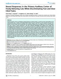
FIG. 1. Optimal prior vs. flat prior reconstruction. A: optimal prior reconstruction (G) is the optimal linear mapping from a population of neuronal responses back to the sound spectrogram (right). Using optimal prior reconstruction, one can reconstruct the spectrogram of a sound, not only features that are explicitly coded by neurons but also features that are correlated with them. Flat prior reconstruction (F) is the best linear mapping of responses to stimulus spectrogram when only the information explicitly encoded by neurons (i.e., their spectro-temporal receptive fields) is known. B: for this simple 3-dimensional system, only x and y values are explicitly encoded in the neural response. Optimal prior reconstruction can reproduce the entire stimulus, using the knowledge that z values are correlated with x and y (in this example, z ⫽ x ⫹ y). However, flat prior reconstruction does not recover information about the data on the z-axis.

J Neurophysiol • VOL

102 • DECEMBER 2009 •

www.jn.org


The two methods for reconstructing the input spectrograms from the neural responses are shown schematically in Fig. 1. In optimal prior reconstruction, we directly estimated the optimal linear mapping from neural responses to the stimulus spectrogram. This method optimally minimizes the mean-squared error (MSE) of the estimated spectrogram. In flat prior reconstruction, we used the neuron’s STRFs to construct a mapping from neural responses to stimulus spectrogram. This method inverts a set of STRFs that are estimated by minimizing the MSE of the predicted neural responses. The optimal prior method and the STRF estimation are the complementary forward and backward predictions in the linear regression framework, and the goodness of the fit is the same for both directions (in terms of the explained fraction of variance, R2) (Draper and Smith 1998). Despite the structural similarities, there are significant conceptual differences between the two methods. One main difference between the two is inclusion and exclusion of known statistical structure of the input in the reconstruction. Because stimulus correlations are removed during ⫺1 STRF estimation (Css in Eq. 5), flat prior reconstruction has no access to stimulus statistics. The optimal prior method, in contrast, uses whatever stimulus correlations are available to improve reconstruction accuracy, even if the information is not explicitly encoded in neural responses. Figure 1B shows this point intuitively. In this example, data are located in three-dimensional (3D) space (xyz), but the STRF response projects them onto the xy plane. Clearly, one dimension of the input (z) is lost in this transformation, and we cannot accurately reconstruct the points in 3D by having only their projections (neural response) and knowledge of the STRFs (flat prior method, F). However, because there is correlation between z and the other two dimensions (in this example, all the points belong to a plane z ⫽ x ⫹ y), having access to this prior knowledge in addition to the STRFs and neural responses enables the correct reconstruction of the points in 3D (optimal prior, G).

To make unbiased measurements of the accuracy of reconstruction, a subset of validation data was reserved from the data used for estimating the reconstruction filter, (G for optimal prior reconstruction or F for flat prior reconstruction). The estimated filter was used to reconstruct the stimulus in the validation set, and reconstruction accuracy was measured in two ways: 1) correlation coefficient (Pearson’s r) between the reconstructed and original stimulus spectrogram and 2) mean squared error. In addition to measuring global reconstruction error for TORCs, we also measured error separately for different parts of the modulation spectrum (i.e., separately for different rates and spectral scales). To do this, we subtracted the reconstructed TORC spectrogram from the original spectrogram and computed the modulation spectrum of the difference. The normalized error for specific rates and scales was defined as the mean squared magnitude of the error modulation spectrum, averaged only over the desired range of rates or scales. Because stimuli were reconstructed from a finite number of neurons and a finite amount of fit data, we also measured the effect of limited sampling on reconstruction performance. For a set of N neurons and T seconds of fit data, the reconstruction error can be attributed to two sources: failure of the neural response to encode stimulus features and error from limited sampling of the neural population and fit data. If we assume that the sources of error are additive, as N and T grow larger, the error from limited sampling should fall off inversely with N and T. To determine reconstruction error in the absence of noise, we measured error, e, for a range of values of N and T and fit the function (David and Gallant 2005)


In the limit of infinite sampling, any remaining reconstruction error reflects stimuli that are either not encoded by the neural population or stimuli that are encoded nonlinearly in such a way that the linear reconstruction filter cannot capture them. Because of the diversity of nonlinear responses across neurons, this latter category is likely to be small; thus in practice, reconstruction error can be interpreted as reflecting stimuli that simply are not encoded.

Effect of behaviorally driven plasticity on reconstructions During behavior, the functional relationship between stimulus and neural response can change to facilitate behavior (Fritz et al. 2003), e.g., through top-down attentional influences that change the gain or shape of the receptive field. To understand how these changes affect reconstruction, consider the receptive field formulation R ⫽ H TS where S is the stimulus, H is the matrix of neural receptive fields, and R is the population response. Because the model is linear, if there is a change in the receptive field, ⌬H, it results in a change, ⌬R, in the neural response

Rather than modeling the change in the receptive field, we assume that the system has not changed and instead find the effective stimulus change that produces the observed change in the neural response ⌬R ⫽ H T⌬S The effective stimulus change (⌬Sˆ) can be found using reconstruction ⌬Sˆ ⫽ G⌬R where G is the optional reconstruction filter measured before the change. In effect, this approach enables us to project response changes (⌬R) to the stimulus domain where they may be more intuitive to interpret. This analysis can also be conceptualized as describing how a downstream decoder would interpret activity from a plastic population of neurons if it uses a fixed decoding scheme. Although this approach is limited to identifying changes in linear response properties, it may provide a means to characterize plasticity that cannot easily be observed in the tuning of individual neurons. We performed this analysis using both simulated and actual neural data for a task that requires discriminating a pure tone target from a sequence of TORC reference sounds. In the simulation, we used a bank of STRFs narrowly tuned to different frequencies (passive STRFs). We simulated behavior-driven plasticity by enhancing the tuning of the STRFs to the target frequency for the neurons with best frequency close to the target tone (active STRFs) (Fritz et al. 2003). We found the difference between spectrograms of TORCs reconstructed from the simulated responses of passive and active STRFs. Changes between conditions in each frequency channel were calculated by the mean square of this difference, averaged over time. For the actual neural data, we divided the neural population (62 neurons) into six groups according to their target tone frequencies. We reconstructed TORC spectrograms from passive and active responses in each group and computed the mean squared difference as above. To average across groups, the difference for each group was aligned to have its target frequency at zero and averaged together. The SE was calculated using the jackknife technique with 20 sets each containing 95% of the data (Efron and Tibshirani 1993). J Neurophysiol • VOL

RESULTS

Reconstruction of spectro-temporally modulated noise spectrograms To study the fidelity of auditory encoding by neurons in AI, we reconstructed spectrograms of TORCs from the responses of 256 AI neurons (see METHODS and Klein et al. 2000). The set of 30 TORCs was specially designed to probe the tuning of AI neurons to spectral and temporal modulations in the sound envelope, as shown in Fig. 2A. The fidelity of their reconstruction shows the extent to which information about different spectro-temporal modulations is encoded in cortical responses. Such modulations are the key carriers of information in complex signals such as speech, animal vocalizations, and other natural sounds (Greenberg 1996; Singh and Theunissen 2003). Hence it is important to determine whether AI responses encode them and whether the range encoded matches observed perceptual capabilities. The analysis reported here used optimal prior reconstruction (Eq. 1). Because TORCs contain no linear correlations (although they may contain higher order dependencies, Christianson et al. 2008), the difference between optimal prior reconstruction and flat prior reconstruction is trivial. For the entire set of TORCs, the correlation between the reconstructed and original spectrograms is 0.62 ⫾ 0.009. Figure 2B shows the accuracy of reconstruction for different spectral and temporal modulation channels. Reconstruction error in the combined modulation spectrum of the TORCs had a low pass structure that could be visualized more clearly when collapsed along its temporal and spectral dimensions (Fig. 2B, right and top panels). Accuracy in the temporal and spectral modulation spectrum was greatest for low modulation frequencies (Fig. 2, C and D). The regions of smallest error represent spectro-temporal features that are encoded with the greatest fidelity in AI. These regions are consistent with patterns of perceptual modulation sensitivity measured in ferrets (Fritz et al. 2002). They also correspond to the region of the modulation spectrum that contains the most energy in natural sounds (Singh and Theunissen 2003). Effect of sample size on reconstruction accuracy Neurons in AI vary substantially in their spectro-temporal tuning properties. A single neuron will respond only to a narrow range of the spectro-temporal patterns in TORCs (Eggermont and Ponton 2002). It was therefore expected that many neurons would be required to achieve a full coverage of the stimulus and that increasing the number of neurons used for reconstruction would improve its accuracy. In addition, reconstruction error was also caused by the finite duration of stimulus-response samples available for estimation. To measure the effects of sampling limitations, we varied the number of neurons used for reconstruction and the duration of fit data and measured the corresponding normalized reconstruction error (see METHODS). In the limit of infinite sampling, the extrapolated error indicates how much information about the stimulus is encoded in the neural population response (David and Gallant 2005). Figure 2C shows the reconstruction error for different temporal and spectral modulation ranges as the number of neurons (N) and stimulus duration (T) increases. As expected for

102 • DECEMBER 2009 •

www.jn.org


⌬R ⫽ ⌬H TS

3333

3334


A

B

|FFT|2 0.5 0

250 Time (ms)

1.4

0

-48 0 48 Temporal modulation (Hz)

C

Spectral modulation (cycles/octave)

16

Spectral modulation (cycles/octave)

Frequency (kHz)

1 0

0

1

1.2 0.8 0.4 0 −48 −4 4 48 Temporal modulation (Hz)

0

D Spectral modulations

0.4 0.2 30

0

60 Time (s)

100 200 its) 90 300 s (un n o r Neu

40−48Hz 28−36Hz 16−24Hz 4−12Hz

1 0.8 0.6 0.4 0.2 0

1 64 128 256 Inf Number of Neurons

Normalized MSE

0.6

1 0.8 0.6 0.4

1.2−1.4 c/o 0.8−1.0 c/o 0.4−0.8 c/o 0.0−0.2 c/o

0.2 0

Inf 1 64 128 256 Number of Neurons

FIG. 2. Reconstruction of broadband noise stimuli. Temporally orthogonal ripple combinations (TORCs) are specially constructed broadband modulated noise stimuli. A: example of a TORC: In each of 30 different TORCs used for reconstruction, the stimulus consists of the superposition of the envelopes of 6 ripples, all at the same ripple density (0.2, 0.4 . . . 1.2 or 1.4 cyc/octave) and ripple velocities from 4 to 48 and ⫺4 to ⫺48 Hz. Thus the 2-dimensional modulation spectrum (MS) of each TORC is a line at a particular spectral modulation density. B: reconstruction error of MTF (modulation transfer function). The MS of the reconstruction error for all TORCs and from all neurons shows better reconstruction accuracy at lower temporal (top) and spectral modulation frequencies (right). C: reconstruction error for N and T. Normalized reconstruction error as a function of the number of neurons and duration of fit data used for estimation. The reconstruction error converges to lower values for lower temporal and spectral modulations. D: reconstruction error for N and T ⫽ inf. Normalized reconstruction error for different temporal and spectral modulations as a function of neuron number after extrapolation to infinite fit data for each neuron.

additive noise, reconstruction error is inversely proportional to N and T. The normalized error averaged across random subsets for different rates and scales for each N is plotted in Fig. 2D. These curves were estimated from Eq. 7, assuming the duration of estimation data (T) was infinite. We used the measurements for variable N to extrapolate to the error that would be expected for arbitrarily large N. The limit of the reconstruction error differs across modulation channels. For slow temporal modulations (4 –12 Hz), the error converges to substantially lower values than for the fast rates (40 – 48 Hz). A similar, although smaller, difference can be seen between low (0 – 0.8 c/o) versus high (1.2–1.4 c/o) scales. A likely reason for the higher bounds at high rates and scales is the loss of encoded information as cortical neurons fail to phase-lock to these faster and denser modulations. Comparison of optimal prior versus flat prior speech reconstruction TORCs are designed to have minimal spectro-temporal correlations (Klein et al. 2000), and therefore reconstructing TORC spectrograms cannot take advantage of prior knowledge of stimulus statistics to improve reconstruction accuracy. However, for natural stimuli such as speech, which do contain strong correlations, this information provides context that can be used to infer features in the stimulus that are not explicitly J Neurophysiol • VOL

coded in the neural responses. The extra information available in stimulus correlations suggests two alternative strategies for reconstruction (detailed in METHODS): optimal prior reconstruction, which assumes knowledge of stimulus correlations, and flat prior reconstruction, which does not. We first examined how prior knowledge of stimulus statistics can improve reconstructed continuous speech spectrograms from simulated responses of a sparse sample of neurons. We simulated the responses of eight neurons that were narrowly tuned and widely spaced across the frequency axis. We reconstructed the spectrogram of one speech sample using the two methods, as shown in Fig. 3, B and C. Optimal prior reconstruction (Fig. 3B) produced a spectrogram closely resembling the original, with a correlation of 0.82. Flat prior reconstruction (Fig. 3C) resulted in a sparse reconstruction with no data in the channels of the spectrogram that were not explicitly encoded by the neurons. In this case, the correlation of the reconstructed and original spectrograms fell to 0.70. The two methods in this example provide us with complementary results: the optimal prior reconstruction demonstrates that, for a highly structured stimulus such as speech, substantial details of the stimulus can be inferred from partially encoded features. The flat prior reconstruction, on the other hand, shows the actual encoding scheme of the system by showing only the features of the stimulus that are explicitly encoded in the neural population response.

102 • DECEMBER 2009 •

www.jn.org


Normalized MSE

Temporal modulations Normalized MSE

1

Frequency (KHz) Frequency (KHz)

C

8 4 2 1 0.5

8 4 2 1 0.5

Frequency (KHz)

B

D Original

8 4 2 1 0.5

0

1

Time (s)

2

3

E

Simulation - Optimal prior (c=0.83)

0

1

Time (s)

2

0

1

Time (s)

3

12 8 4 0 0.2 0.4 0.6 0.8 1 Correlation with original

3335

0.8 0.6 0.4 0.2 0.2 0.4 0.6 0.8 Flat prior (F)

Neural data - Optimal prior (c=0.78)

F

2

Flat prior (F) Optimal prior (G)

0

3

Simulation - Flat prior (c=0.70)

16

Optimal prior (G)

A

Number of sentences


1

Time (s)

2

3

2

3

Neural data - Flat prior (c=0.42)

0

1

Time (s)

To contrast optimal and flat prior reconstruction using experimental data, we reconstructed the spectrograms of speech from the responses of 250 AI neurons. The population response to the same speech stimuli was used to estimate optimal and flat prior reconstructions. Figure 3 shows an example of one speech sentence (Fig. 3A) and its reconstructions using the optimal prior (Fig. 3E) and flat prior (Fig. 3F) methods. The optimal prior reconstruction was superior to that of the flat prior method, as judged by its higher correlation with the original stimulus spectrogram (0.78 vs. 0.42). When we compared performance of the two methods for all 30 sentences (Fig. 3D), we observed the same consistent result. In every case, the optimal prior reconstruction always had a higher correlation (mean, 0.75) with the original spectrogram than the flat prior reconstruction (mean, 0.45). The consistently superior performance of the optimal prior reconstruction shows the benefit of prior knowledge on the decoding of stimulus information from neural responses. Together, they define upper and lower bounds on what aspects of the stimulus an animal might perceive, at one extreme, using no prior information and, at the other, using optimal prior information. To compare the perceptibility of these reconstructions, we inverted the spectrograms to generate the best approximation of corresponding acoustic signals using a convex projection method (Chi et al. 2005). Audio examples of reconstructions using optimal prior reconstruction were noticeably more clear than those reconstructed with a flat prior (AudioSamples). Reconstructed phonemes from neural population responses To what extent do responses of auditory cortical neurons in the ferret encode phonemes with enough fidelity to account for their perception in humans? This question implicitly tests the hypothesis that auditory processing mechanisms up to the level of the primary auditory cortex, common across humans and J Neurophysiol • VOL

other mammals like ferrets, are sufficient to account for the robust perception of speech (Greenberg et al. 2004; Mesgarani et al. 2008; Steinschneider et al. 2005). Previous analyses of AI responses in mammals have been consistent with this point of view (Engineer et al. 2008; Mesgarani et al. 2008). Here we used the reconstruction method to shed more light on this issue and compare, in particular, reconstruction accuracy and the pattern of errors observed in the perception of various phonemes by humans. We first analyzed the encoding of the average spectrotemporal features of each phoneme in the population response. Figure 4, A–D (top rows), shows the average phoneme spectrograms of four groups of phonemes (plosives, fricatives, nasals, and vowels) extracted from the continuous speech samples using the phonetic transcriptions detailed in Mesgarani et al. (2008). The corresponding panels in the bottom rows of Fig. 4, A–D, depict the average spectrograms of the same phonemes but from reconstructions using optimal prior reconstruction. The strong similarity between the two sets of spectrograms (average correlation coefficient of 0.88 ⫾ 0.07) indicates that average responses of AI neurons have the dynamics and spectral selectivity to linearly encode most details of the average spectro-temporal features of phonemes. Comparing only the average phoneme spectrograms improves accuracy performance by averaging out differences between phoneme exemplars. To make a more critical assessment of the results, we examined the accuracy of reconstructions for each phoneme exemplar separately. Figure 4E plots the average reconstruction error across all instances of each phoneme. Some phonemes, such as the high-frequency fricatives (/s/, /兰/, /z/, /f/) (Ladefoged 2005), show excellent reconstruction accuracy even at the level of individual exemplars (average normalized error, 0.5). Most plosives (/p/, /b/, /t/, /d/, /k/, /g/) are encoded with an intermediate level of accuracy

102 • DECEMBER 2009 •

www.jn.org


FIG. 3. Comparison of optimal prior and flat prior reconstruction in simulations and with physiological data. A: original spectrogram of a speech sample. B: optimal prior reconstruction of the speech spectrogram from simulated responses of 8 neurons that were spectrally narrowly tuned and widely spaced produced a reasonably complete spectrogram. C: flat prior reconstruction using the same neurons as in B results in a sparser spectrogram with gaps between the explicitly encoded frequency channels. D: comparison of the accuracy of optimal prior and flat prior reconstruction for 30 different sentences using physiological responses of auditory cortex (AI) 250 neurons. The distribution of the correlation coefficients for optimal prior reconstruction was consistently higher than that for the flat prior method. E: example of optimal prior reconstruction of 1 sentence from physiological data. F: flat prior reconstruction using the same data produces a less accurate match to the original spectrogram.

3336


A t

Frequency (KHz)

p

b

k

d

f

s

ʃ

v

z

t

b

k

d

f

s

ʃ

v

z

g

0.25

0.25

0.25 0

170

0

170

0

170 0 170 Time (ms)

0

170

0

170

0

170

0

170

0 170 0 Time (ms)

170

Frequency (KHz)

8

0.25

o

ɑ

ɔ

ɑ

ʌ

æ

ʌ

æ

ə

e

ɛ

ə

e

ɛ

i

i

ɪ

170 0

170

0

170 0

170 0

170 0 170 Time (ms)

n

ŋ

170

0

Closed Vowels

i

ɪ

1

i

0.25 0

0

Normalized MSE

Frequency (KHz)

8

ɔ

m

170

0 170 0 Time (ms)

170

E

Vowels o

ŋ

8

8

8

n

0.25

0.25

p

Nasals m

8

8

D Reconstructed Original

C

Fricatives

g

8

0.25

Frequency (KHz)

Reconstructed Original

B

Plosives

0

170 0

170

0

170 0

170

0

170

0.9 0.8 0.7 0.6 0.5

iu

iə

oɪ

nv ʌ g

Open Vowels

pŋb ɛd mæ t

Vowels Plosives Fricatives Nasals

ke ɑf ɔ z ʃs

0.4

(average normalized error, 0.65). In general, the close-front vowels (e.g., /i/) with low first and high second formant frequencies (Ladefoged 2005) show a worse reconstruction accuracy that the open-back ones (e.g., /ɔ/). This may be because of the more complex spectral shape of the former group, which has multiple peaks compared with the single spectral peak of the latter. The sometimes low and variable accuracy of the reconstructions for individual phoneme exemplars stands in striking contrast to the highly accurate encoding of the average features (Fig. 4, A–D). Averaging of spectrograms across all instances of a phoneme preserved only features that were common across all syllabic contexts and hence not affected by co-articulatory factors. These common features were generic enough to be captured well by the linear spectro-temporal response models in AI. In contrast, the unique features of individual phoneme samples were sometimes not well described by the reconstruction. Stimulus reconstruction and neural plasticity Receptive field properties in AI can rapidly change during task performance in accordance with specific task demands and salient sensory cues (Fritz et al. 2003). Such rapid plasticity may reflect changes in coding strategy to enhance representations of stimuli relevant to the task. Previously, these changes have been characterized with single neurons and extrapolated to predict consequences for the population code (Fritz et al. 2007; McAdams and Maunsell 1999). In go/no-go tasks requiring simple discrimination (e.g., tone vs. noise), changes in spectro-temporal tuning enhance overall cortical responsiveness to a foreground (or target) sound while suppressing responsiveness to the background (or reference) sound, presumably increasing the likelihood of detecting the attended target (Fritz et al. 2003, 2005). However, as the complexity of auditory discrimination increases (e.g., when discriminating among phonemes, tonal J Neurophysiol • VOL

sequences, or musical timbres), receptive field changes are likely to become more complex and hence more challenging to relate to the acoustical properties of the stimuli. Another limitation of the traditional approach of examining the plasticity of neurons in isolation is that it does not benefit from multielectrode recordings. Changes across an entire population may be easier to detect than in single neurons. Both of these limitations can be addressed by a reformulation of the analysis of plasticity using stimulus reconstruction. We evaluated this approach first using simulated receptive field changes, based on observations from behavioral physiology experiments that used a tone detection task (Fig. 5) (Fritz et al. 2003). The reconstructions considered here were those of TORC stimuli before behavior, when neurons are in a baseline state, and during behavior, when neurons have undergone a change in tuning. As stated earlier, here we used optimal prior reconstruction; however, because this analysis involved uncorrelated noise stimuli, there was no practical difference from flat prior reconstruction. The simulated neurons constituted a bank of tonotopically distributed filters, represented by the three STRFs in the left column of Fig. 5A, centered at the different frequencies. During behavior, the target tone was played at 3 KHz, which caused the nearby STRFs (at 3 and 4 KHz) to expand toward the target or become more sensitive to it (Fig. 5A, right column). This plasticity induces 3-KHz responses to become more correlated with its neighboring channels. Figure 5B shows the reconstructed TORC stimuli before (top panel) and during the task (middle panel). The changes are best seen in the difference (⌬S) between two reconstructions (Fig. 5B, bottom). The mean-squared difference (averaged over time) between active and passive reconstructions is shown in the top panel of Fig. 5C. The peak difference occurs at the target frequency. We applied the reconstruction analysis to physiological data recorded from AI, which showed STRF plasticity similar to the simulations above (Fritz et al. 2003). We divided the neural

102 • DECEMBER 2009 •

www.jn.org


FIG. 4. Average phoneme spectrograms from original and reconstructed phonemes. A–D: top: the average phoneme spectrograms of 4 groups of phonemes (plosives, fricatives, nasals, and vowels). Bottom: corresponding panels depict the average phoneme spectrograms reconstructed using the optimal prior method. The original and reconstructed spectrograms are quite similar and have an average correlation coefficient of 0.88. E: the correspondence between reconstructions and actual spectrograms for each phoneme exemplar, averaged across all instances of the phoneme.


A

B passive

active

0.5 frequency (KHz)

frequency (KHz)

3

3 0.5 16

Target

Simulated average difference

16

0.5 16 Target

C Reconstructed passive TORC

16 Target

3337

Reconstructed active TORC

16

-2

Target

-1

0

1

2

Neural average difference 0.5

Difference spectrogram 16

3

Target

0.5 0

0.25

0

0.25

Time (s)

0.5

0

1 Time (s) 2

3

-2

-1 0 1 2 Octave from target

population into six groups, according to the frequency of the target tone, and measured the average mean-squared difference between spectrograms reconstructed from responses before and during behavior (Fig. 5C, bottom). To average across groups, data from each of the six groups was centered at the target frequency and weighted according to the number of neurons in the group. As predicted by the simulation, the difference between reconstructions contains a peak at the target frequency (red bar), indicating that a significant shift occurred in the population response to stimuli at the target frequency. DISCUSSION

Characteristics of the AI population code Beyond their overall fidelity, stimulus reconstructions indicate the limits, tuning, and specific features encoded in the cortical population response. We found that the accuracy of encoding by the population of AI neurons is better for low scales and rates, and the accuracy falls off for higher rates and scales, especially rates greater than ⬃30 Hz. However, some information about modulations is encoded, even ⱕ50 Hz and 1.4 c/o. The most accurately reconstructed spectro-temporal features lie in the region of the modulation spectrum that contains the most power in natural sounds (Singh and Theunissen 2003), suggesting that the population code in auditory cortex matches the regions of maximum information in stimuli that are encountered in the world. The method of reconstruction allows for the assessment of the upper bound on coding accuracy for any stimulus while controlling for potential confounds that can occur in other metrics, such as ensemble tuning curves (Woolley et al. 2005). As the number of neurons used for reconstruction increases, any persistent error in reconstruction reflects the aspects of the stimuli that are not encoded in the neural responses. By J Neurophysiol • VOL

judicious choice of stimuli, one can interrogate the ability of neurons to encode any number of stimulus parameters. The example we presented of the encoding of TORC spectral and temporal modulations is but one that is appropriate for AI cells, which are modulated over a range of rates and spectral densities (Kowalski et al. 1996). The same approach may also be beneficial in precortical areas that follow stimulus modulations at higher rates. This same general approach can be applied to areas outside of the auditory system. Rather than reconstructing the stimulus spectrogram, one can parameterize the stimulus in terms of other features that are correlated with neuronal responses. Such an approach is similar to methods for decoding movements from the population response in the motor system (Georgopoulos et al. 1986). In the visual system, reconstruction methods could be used to measure coding of features such as orientation, spatial frequency, and phase (Mazer et al. 2002). In more central areas, this approach could be used to measure coding of abstract and learned stimulus features (Wallis and Miller 2003). Encoding of complex natural features An appealing aspect of reconstruction methods is the mapping of potentially complex acoustic features from the neural response back to the stimulus space, where they can be displayed intuitively. Speech is a prime example of a stimulus where much has been learned over the decades about its acoustic features almost exclusively in the spectrogram (timefrequency) representation (Greenberg et al. 2004). It is, of course, possible to explore the encoding of known features such as plosive bursts and voice-onset-times (Eggermont and Ponton 2002; Steinschneider et al. 2005), but this procedure requires manually identifying features and provides less general insight than the reconstructed spectrograms—where these

102 • DECEMBER 2009 •

www.jn.org


FIG. 5. Detecting spectro-temporal tuning changes in simulated and actual neural data. A: simulated spectro-temporal receptive fields (STRFs) undergoing changes that might occur during behavioral experiments. Left column: during passive stimulation before the behavioral experiment, 3 STRFs are tuned to different frequencies centered at 3, 4, and 7 KHz. The target tone during the experiment is at 3 KHz. Right column: during behavior, the STRF closest to the target tone becomes more sensitive to the target tone by broadening its excitatory field toward the target frequency. B: reconstructed TORCs using passive (top) and active (middle) simulated responses. The change in the STRF at 3 KHz causes the TORC reconstruction to change locally, which can be detected by subtracting the 2 TORC spectrograms (bottom). C: top: mean-squared difference (averaged over time) between active and passive simulated spectrograms with the peak difference at the target frequency (red bar). Bottom: the average mean squared difference between spectrograms reconstructed from actual neural responses before and during behavior. The error was calculated separately for 6 groups of neurons (grouped according to target frequency) and aligned at the target frequency before averaging. As in the simulation, the difference between reconstructions contains a peak at the target frequency (red bar).

3338


features were defined in the first place. By studying the representation of speech directly in the spectrogram domain, it is possible to simultaneously study the encoding of many spectral and temporal features. Optimal prior reconstruction (Bialek et al. 1991) was contrasted with flat prior reconstruction to measure how knowledge of stimulus context can benefit reconstruction. In natural stimuli, including speech, animal vocalizations, and music, significant correlations exist across a wide range of time and frequencies. An effective and efficient encoding scheme reduces this redundant information to conserve resources (Barlow 1972). We found that reconstructions that make use of these priors generate substantially more accurate reconstructions for the same number of responses than is possible with the flat prior method. In practice, the prior actually used during perception remains largely unexplored. Thus the flat prior reconstruction represents a lower bound on the accuracy with which stimuli are encoded. Characterizing the prior actually used by animals will require further study, perhaps using a behavioral approach that measures the ability to detect stimuli based on correlated features. Interpreting adaptive STRFs

ACKNOWLEDGMENTS

We thank two anonymous reviewers for valuable comments. GRANTS

This work was supported by National Institute of Deafness and Other Communication Disorders Grants R01-DC-005779 and F32-DC-008453 and J Neurophysiol • VOL

REFERENCES

AudioSamples. www.ee.umd.edu/⬃mnima/Reconstruction. Barlow HB. Single units and sensation: a neuron doctrine for perceptual psychology? Perception 1: 371–394, 1972. Bialek W, Rieke F, de Ruyter van Steveninck RR, Warland D. Reading a neural code. Science 252: 1854 –1857, 1991. Buracas GT, Zador AM, DeWeese MR, Albright TD. Efficient discrimination of temporal patterns by motion-sensitive neurons in primate visual cortex. Neuron 20: 959 –969, 1998. Butts DA, Goldman MS. Tuning curves, neuronal variability, and sensory coding. PLoS Biol 4: e92, 2006. Chi T, Ru P, Shamma SA. Multiresolution spectrotemporal analysis of complex sounds. J Acoust Soc Am 118: 887–906, 2005. Christianson GB, Sahani M, Linden JF. The consequences of response nonlinearities for interpretation of spectrotemporal receptive fields. J Neurosci 28: 446 – 455, 2008. David SV, Gallant JL. Predicting neuronal responses during natural vision. Network 16: 239 –260, 2005. de Ruyter van Steveninck RR, Lewen GD, Strong SP, Koberle R, Bialek W. Reproducibility and variability in neural spike trains. Science 275: 1805–1808, 1997. De Valois RL, Yund EW, Hepler N. The orientation and direction selectivity of cells in macaque visual cortex. Vision Res 22: 531–544, 1982. Draper NR, Smith H. Applied Regression Analysis. New York: Wiley, 1998. Efron B, Tibshirani R. An Introduction to the Bootstrap. New York: Chapman and Hall, 1993. Eggermont JJ, Ponton CW. The neurophysiology of auditory perception: from single units to evoked potentials. Audiol Neurootol 7: 71–99, 2002. Engineer CT, Perez CA, Chen YH, Carraway RS, Reed AC, Shetake JA, Jakkamsetti V, Chang KQ, Kilgard MP. Cortical activity patterns predict speech discrimination ability. Nat Neurosci 11: 603– 608, 2008. Ferragamo MJ, Haresign T, Simmons JA. Frequency tuning, latencies, and responses to frequency-modulated sweeps in the inferior colliculus of the echolocating bat, Eptesicus fuscus. J Comp Physiol [A] 182: 65–79, 1998. Fritz J, Bozak D, Depireux DA, Dobbins H, Tillman A, Shamma SA. Measuring the ferret spectro-temporal transfer function (MTF) using a conditioned behavioral task. In: Association for Research in Otolaryngology, 2002, Abs.: 802. Fritz J, Shamma S, Elhilali M, Klein D. Rapid task-related plasticity of spectrotemporal receptive fields in primary auditory cortex. Nat Neurosci 6: 1216 –1223, 2003. Fritz JB, Elhilali M, David SV, Shamma SA. Does attention play a role in dynamic receptive field adaptation to changing acoustic salience in A1? Hear Res 229: 186 –203, 2007. Fritz JB, Elhilali M, Shamma SA. Differential dynamic plasticity of A1 receptive fields during multiple spectral tasks. J Neurosci 25: 7623–7635, 2005. Garofolo JS, Lamel LF, Fisher WM, Fiscus JG, Pallett DS, Dahlgrena NL, Zue V. TIMIT Acoustic-Phonetic Continuous Speech Corpus. Linguistic Data Consortium, 1993. Georgopoulos AP, Schwartz AB, Kettner RE. Neuronal population coding of movement direction. Science 233: 1416 –1419, 1986. Gielen CCAM, Hesselmans GHFM, Johannesma PIM. Sensory interpretation of neural activity patterns. Math Biosci 88: 15–35, 1988. Greenberg S. Understanding speech understanding: toward a unified theory of speech perception. Proceedings of the ESCA Tutorial and Advanced Research Workshop on the Auditory Basis of Speech Perception. Keele, England, 1996 p. 1– 8. Greenberg S, Ainsworth WA, Popper AN, Fay RR. Speech Processing in the Auditory System. New York: Springer-Verlag, 2004, vol. 18. Haag J, Borst A. Active membrane properties and signal encoding in graded potential neurons. J Neurosci 18: 7972–7986, 1998. Han YK, Kover H, Insanally MN, Semerdjian JH, Bao S. Early experience impairs perceptual discrimination. Nat Neurosci 10: 1191–1197, 2007. Hesselmans GH, Johannesma PI. Spectro-temporal interpretation of activity patterns of auditory neurons. Math Biosci 93: 31–51, 1989. Klein DJ, Depireux DA, Simon JZ, Shamma SA. Robust spectrotemporal reverse correlation for the auditory system: optimizing stimulus design. J Comput Neurosci 9: 85–111, 2000.

102 • DECEMBER 2009 •

www.jn.org


A potentially exciting deployment of stimulus reconstruction is in detecting and interpreting behaviorally driven changes in response properties. We found that, during a tone detection task, changes in tuning at the frequency of the target tone can be shown by the trace they induce in the difference between original and reconstructed spectrograms. One can extrapolate from this simple example to more intricate situations where top-down influences such as attention, expectation, or memory might modify receptive field shapes. For instance, changes induced in detecting an amplitude-modulated target tone or a specific phoneme might span many frequencies and time lags. These changes could be expressed differently in each STRF, depending on its BF (best frequency) and other baseline spectro-temporal properties, but they may have a systematic effect on the reconstructed stimulus. This approach may be particularly valuable for behaviors requiring the discrimination of temporal features, where no systematic changes have yet been identified in STRFs or tuning curves, despite the importance of temporal processing for many auditory behaviors (Shannon et al. 1995). Because this method only identifies stimulus domains where plasticity occurs, it does not completely characterize the effects of plasticity. However, it offers a new way to visualize and understand the effects of behavior on neural representations. Simultaneous recordings from large assemblies of primary cortical neurons may provide additional insight into changes in stimulus representation. Features of population responses such as correlated firing may have substantial impact on how stimuli are encoded and how this coding changes during behavior (Salinas and Sejnowski 2001). This possibility suggests a means to interpret large simultaneous neural recordings during behavior in the future.

the Air Force Office of Scientific Research through a subcontract with Advanced Acoustic Concepts.


J Neurophysiol • VOL

Shamma SA. Speech processing in the auditory system. I. The representation of speech sounds in the responses of the auditory nerve. J Acoust Soc Am 78: 1612–1621, 1985. Shannon RV, Zeng FG, Kamath V, Wygonski J, Ekelid M. Speech recognition with primarily temporal cues. Science 270: 303–304, 1995. Singh NC, Theunissen FE. Modulation spectra of natural sounds and ethological theories of auditory processing. J Acoust Soc Am 114: 3394 –3411, 2003. Stanley GB, Li FF, Dan Y. Reconstruction of natural scenes from ensemble responses in the lateral geniculate nucleus. J Neurosci 19: 8036 – 8042, 1999. Steinschneider M, Volkov IO, Fishman YI, Oya H, Arezzo JC, Howard MA III. Intracortical responses in human and monkey primary auditory cortex support a temporal processing mechanism for encoding of the voice onset time phonetic parameter. Cereb Cortex 15: 170 –186, 2005. Theunissen FE, David SV, Singh NC, Hsu A, Vinje WE, Gallant JL. Estimating spatio-temporal receptive fields of auditory and visual neurons from their responses to natural stimuli. Network 12: 289 –316, 2001. Wallis JD, Miller EK. Neuronal activity in primate dorsolateral and orbital prefrontal cortex during performance of a reward preference task. Eur J Neurosci 18: 2069 –2081, 2003. Warland DK, Reinagel P, Meister M. Decoding visual information from a population of retinal ganglion cells. J Neurophysiol 78: 2336 –2350, 1997. Woolley SM, Fremouw TE, Hsu A, Theunissen FE. Tuning for spectrotemporal modulations as a mechanism for auditory discrimination of natural sounds. Nat Neurosci 8: 1371–1379, 2005. Yang XWK, Shamma SA. Auditory representations of acoustic signals. IEEE Trans Inform Theory 38: 824 – 839, 1992.

102 • DECEMBER 2009 •

www.jn.org


Kowalski N, Depireux DA, Shamma SA. Analysis of dynamic spectra in ferret primary auditory cortex. I. Characteristics of single-unit responses to moving ripple spectra. J Neurophysiol 76: 3503–3523, 1996. Ladefoged P. Course in Phonetics. Heinle. Orlando: Harcourt Brace, 2005. Mazer JA, Vinje WE, McDermott J, Schiller PH, Gallant JL. Spatial frequency and orientation tuning dynamics in area V1. Proc Natl Acad Sci USA 99: 1645–1650, 2002. McAdams CJ, Maunsell JH. Effects of attention on orientation-tuning functions of single neurons in macaque cortical area V4. J Neurosci 19: 431– 441, 1999. Mesgarani N, David SV, Fritz JB, Shamma SA. Phoneme representation and classification in primary auditory cortex. J Acoust Soc Am 123: 899 –909, 2008. Miyawaki Y, Uchida H, Yamashita O, Sato MA, Morito Y, Tanabe HC, Sadato N, Kamitani Y. Visual image reconstruction from human brain activity using a combination of multiscale local image decoders. Neuron 60: 915–929, 2008. Rieke F, Bodnar DA, Bialek W. Naturalistic stimuli increase the rate and efficiency of information transmission by primary auditory afferents. R Soc Lond Ser B 262: 259 –265, 1995. Sachs MB, Young ED. Encoding of steady-state vowels in the auditory nerve: representation in terms of discharge rate. J Acoust Soc Am 66: 470 – 479, 1979. Salinas E, Sejnowski TJ. Correlated neuronal activity and the flow of neural information. Nat Rev Neurosci 2: 539 –550, 2001. Schreiner CE, Langner G. Periodicity coding in the inferior colliculus of the cat. II. Topographical organization. J Neurophysiol 60: 1823–1840, 1988. Seneft S, Zue V. Transcription and Alignment of the Timit Database. Edited by Garofolo JS. Gaithersburg, MD: National Institute of Standard and Technology (NIST), 1988.

3339