Automated Edge Detection Using Convolutional Neural Network

(IJACSA) International Journal of Advanced Computer Science and Applications, Vol. 4, No. 10, 2013

Automated Edge Detection Using Convolutional Neural Network Mohamed A. El-Sayed

Yarub A. Estaitia

Mohamed A. Khafagy

Dept. of Math., Faculty of Science, University of Fayoum, Egypt. Assistant prof. of CS, Taif University, KSA

Assistant prof. of Computer Science, College of computers and IT, Taif University, KSA

Dept. of Mathematics, Faculty of Science, Sohag University, Egypt

Abstract—The edge detection on the images is so important for image processing. It is used in a various fields of applications ranging from real-time video surveillance and traffic management to medical imaging applications. Currently, there is not a single edge detector that has both efficiency and reliability. Traditional differential filter-based algorithms have the advantage of theoretical strictness, but require excessive postprocessing. Proposed CNN technique is used to realize edge detection task it takes the advantage of momentum features extraction, it can process any input image of any size with no more training required, the results are very promising when compared to both classical methods and other ANN based methods. Keywords—Edge detection; Convolutional Neural Networks; Max Pooling

I. INTRODUCTION Computer vision aims to duplicate the effect of human vision by electronically perceiving and understanding an image. Giving computers the ability to see is not an easy task. Towards computer vision the role of edge detection is very crucial as it is the preliminary or fundamental stage in pattern recognition. Edges characterize object boundaries and are therefore useful for segmentation and identification of objects in a scene. The idea that the edge detection is the first step in vision processing has fueled a long term search for a good edge detection algorithm [1]. Edge detection is a crucial step towards the ultimate goal of computer vision, and is an intensively researched subject; an edge is defined by a discontinuity in gray level values. In other words, an edge is the boundary between an object and the background. The shape of edges in images depends on many parameters: The geometrical and optical properties of the object, the illumination conditions, and the noise level in the images. Edges include the most important information in the image, and can provide the information of the object’s position [2]. Edge detection is an important link in computer vision and other image processing, used in feature detection and texture analysis. Edge detection is frequently used in image segmentation. In that case an image is seen as a combination of segments in which image data are more or less homogeneous. Two main alternatives exist to determine these segments:

1) Classification of all pixels that satisfy the criterion of homogeneousness; 2) Detection of all pixels on the borders between different homogeneous areas. Edges are quick changes on the image profile. These quick changes on the image can be detected via traditional difference filters [3]. Also it can be also detected by using canny method [4] or Laplacian of Gaussian (LOG) method [5]. In these classic methods, firstly masks are moved around the image. The pixels which are the dimension of masks are processed. Then, new pixels values on the new image provide us necessary information about the edge. However, errors can be made due to the noise while mask is moved around the image [6]. The class of edge detection using entropy has been widely studied, and many of the paper , for examples [7],[8],[9]. Artificial neural network can be used as a very prevalent technology, instead of classic edge detection methods. Artificial neural network [10], is more as compared to classic method for edge detection, since it provides less operation load and has more advantageous for reducing the effect of the noise [11]. An artificial neural network is more useful, because multiple inputs and multiple outputs can be used during the stage of training [12], [13]. Many edge detection filters only detect edges in certain directions; therefore combinations of filters that detect edges in different directions are often used to obtain edge detectors that detect all edges. This paper is organized as follows: Section 2 presents some fundamental concepts and we describe the proposed method used. In Section 3, we report the effectiveness of our method when applied to some real-world and some standard database set of images. At last Results, Discussion and Conclusion of this paper will be drawn in Section 4. II. PIXEL BASED EDGE DETECTION In digital image processing, we can write an image as a set of pixels f p , q and an edge detection filter which detects edges with direction  as a (template) matrix with elements wn ,m , see Figure.1. We can then determine whether a pixel f p , q is an edge pixel or not, by looking at the pixel’s neighborhood, see Figure 2, where the neighborhood has the same size as the

11 | P a g e www.ijacsa.thesai.org


edge detector template, say (2 N  1)  (2M  1) . We then calculate the discrete convolution.

g p,q 

N

M

 w

n N m M

n,m

f p n,q  m

(1)

where f p , q can be classified as an edge pixel if g p ,q exceeds a certain threshold and is a local maximum in the direction perpendicular to  in the image g p ,q .

 w N ,M  .   .   .  w N ,  M 

.

.

wN , M       wN ,  M 

.

. w0, 0 . .

.

specificity at the same time. Of course, this idea is not new, but the concept is both simple and powerful [15]. It combines three architectural ideas to ensure some degree of shift, scale and distortion invariance: local receptive fields, shared weights (or weights replications), and spatial or temporal sub-sampling [16].

. wn ,m .

Fig. 1. A (2 N  1)  (2M  1) template

Fig. 3. Convolutional Neural Networks structure.

 f  P ,Q  .      .     .   w P , Q

.

.

f P ,Q            .  . wP , Q  .

.

. f p  N ,q  M .

. .

.

.

.

f p  N ,q  M .

f p,q

.

. f p  N ,q  M

.

.

.

.

.

f p  N ,q  M

. .

.

Fig. 2. A (2P  1)  (2Q  1) image with a (2 N  1)  (2M  1) neighborhood around f p , q .

Some examples of templates for edge detection are: -1

-2

-1

1

1

1

0

0

0

0

0

0

1

2

1

-1

-1

-1

,0°

Sobel

, 0°

Prewritt

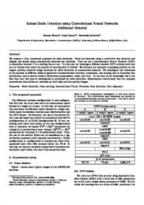
The input plane receive images, each unit in a layer receives input from a set of units located in a small neighborhood in the previous layer. With local receptive fields, neurons can extract elementary visual features such as oriented edges, end points, corners (or other features such as speech spectrograms).These features are then combined by the subsequent layers in order to detect higher-order features. IV. PROPOSED TECHNIQUE Convolutional Neural Networks (Convolutiobal Neural Network) are variants of MLPs which are inspired from biology. From Hubel and Wiesel’s early work on the cat’s visual cortex , we know there exists a complex arrangement of cells within the visual cortex. These cells are sensitive to small sub-regions of the input space, called a receptive field, and are tiled in such a way as to cover the entire visual field. These filters are local in input space and are thus better suited to exploit the strong spatially local correlation present in natural images. Additionally, two basic cell types have been identified: simple cells (S) and complex cells (C). Simple cells (S) respond maximally to specific edge-like stimulus patterns within their receptive field. Complex cells (C) have larger receptive fields and are locally invariant to the exact position of the stimulus. a) Sparse Connectivity: Layer M+1

The dependency on the edge direction  is not very strong; edges with a direction  ± 45° will also activate the edge detector [14]. III. CONVOLUTIONAL NEURAL NETWORKS Typically convolutional layers are interspersed with subsampling layers to reduce computation time and to gradually build up further spatial and configurable invariance. A small sub-sampling factor is desirable however in order to maintain

Layer M Layer M-1

Fig. 4. A Sparse Connectivity template .



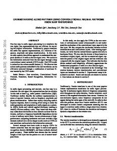
Convolutional Neural Networks exploit spatially local correlation by enforcing a local connectivity pattern between neurons of adjacent layers. The input hidden units in the m-th layer are connected to a local subset of units in the (M -1)-th layer, which have spatially contiguous receptive fields. We can illustrate this graphically as follows: Imagine that layer M-1 is the input retina. In the above, units in layer m have receptive fields of width 3 with respect to the input retina and are thus only connected to 3 adjacent neurons in the layer below (the retina). Units in layer m have a similar connectivity with the layer below. We say that their receptive field with respect to the layer below is also 3, but their receptive field with respect to the input is larger (it is 5). The architecture thus confines the learnt “filters” (corresponding to the input producing the strongest response) to be a spatially local pattern (since each unit is unresponsive to variations outside of its receptive field with respect to the retina). As shown above, stacking many such layers leads to “filters” (not anymore linear) which become increasingly “global” however (i.e. spanning a larger region of pixel space). For example, the unit in hidden layer M +1 can encode a nonlinear feature of width 5 (in terms of pixel space) [17]. b) Shared Weights Neural Network: Hidden units can have shift windows too this approach results in a hidden unit that is translation invariant. But now this layer recognizes only one translation invariant feature, what can make the output layer unable to detect some desired feature. To fix this problem, we can add multiple translation invariant hidden layers: Input

Hidden

Output

Layer

Layer

Layer

A full connected neural network is not a good approach because the number of connections is too big, and it is hard coded to only one image size. At the learning stage, we should present the same image with shifts otherwise the edge detection would happen only in one position (what was useless). Exploring properties of this application we assume: The edge detection should work the same way anywhere the input image is placed. This class of problem is called Translation Invariant Problem. The translation invariant property leads to the question: why to create a full connected neural network? There is no need to have full connections because we always work with finite images .The farther the connection, the less importance to the computation [18]. c) Max Pooling Another important concept of Convolutional Neural Networks is that of max-pooling, which a form of non-linear down-sampling is. Max-pooling partitions the input image into a set of non-overlapping rectangles and, for each such subregion, outputs the maximum value. Max-pooling is useful in vision for two reasons: 1) It reduces the computational complexity for upper layers. 2) It provides a form of translation invariance. To understand the invariance argument, imagine cascading a max-pooling layer with a convolutional layer. There are 8 directions in which one can translate the input image by a single pixel. If max-pooling is done over a 2x2 region, 3 out of these 8 possible configurations will produce exactly the same output at the convolutional layer. For max-pooling over a 3x3 window, this jumps to 5/8. Since it provides additional robustness to position, max-pooling is thus a “smart” way of reducing the dimensionality of intermediate representations [19]. a) graphical depiction of a model: Sparse, Convolutional layers and max-pooling are at the heart of the Convolutional Neural Network models. While the exact details of the model will vary greatly, Figure 6 shows a graphical depiction of a model. Implementing the network shown in Figure 3, the input image is applied recursively to down-sampling layers reduces the computational complexity for upper layers and reduce the dimension of the input, also the network has a 3x3 receptive fields that process the sup sampled input and output the edge detected image, the randomly initialized model acts very much like an edge detector as shown in Figure 7.

Shared

Shared

Weights

Weights

Fig. 5. Shared Weight Neural Network Edit image

The hidden layers activate for partial edge detection, somehow just like real neurons described in Eye, Brain and Vision (EBV) from David Hubel. Probably there is not “shared weights” in brains neurons, but something very near should be achieved with the presentation of patterns shifting along our field of view [20].



Fig. 7. Output of randomly initialized network

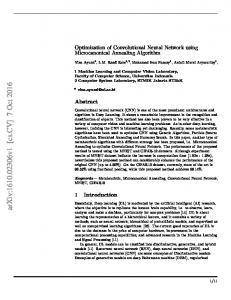
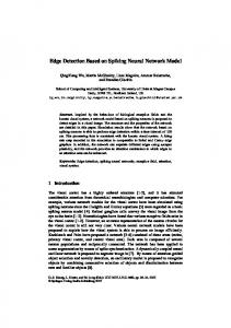
The training of Convolutiobal Neural Networks is very similar to the training of other types of NNs, such as ordinary MLPs. A set of training examples is required, and it is preferable to have a separate validation set in order to perform cross validation and “early stopping” and to avoid overtraining. To improve generalization, small transformations, such as shift and distortion, can be manually applied to the training set. Consequently the set is augmented by examples that are artificial but still form valid representations of the respective object to recognize. In this way, the Convolutiobal Neural Network learns to be invariant to these types of transformations. In terms of the training algorithm, in general, online Error Backpropagation leads to the best performance of the resulting Convolutiobal Neural Network [21]. The training patterns for the neural network are shown in Figure 8. Totally 17 patterns are considered, including 8 patterns for "edge" and 9 patterns for "non-edge". During training, all 17 patterns are randomly selected. For simplicity, all training patterns are binary images.

Fig. 8. Edge and non edge Training Patterns

V.

EXPERIMENT DISCUSSION

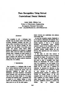
The training process passes many stage according to training epoch's number to reach the weight values that gives the best result, the epoch's number value ranges from 100 epoch to 100000 epoch as a maximum number performed. The PSNR (peak signal-to-noise ratio) is used to evaluate the network output during raising the epoch's number. The following Figure 9 shows the output result and its PSNR value to a test Lena image at different statuses of epoch's number value. Fig. 6. Full Model of Convolutional Neural network

Figure 9 shows the changes of the edge detected output image of the proposed technique, it is obvious that the best



result that gathers more expected edge pixels with least noise, PSNR = +5.33dB is reached when network was trained 100000 times, what approves the validity and efficiency of our proposed technique, the following Figure 10 shows the changes of the noise ratio in the output edge detected Lena image when applied to the proposed system during increasing the training epochs number from 400 to 100000 epoch, a significant changes occurred when we raised the epoch number to its maximum value.

Original Image

epochs =400,

epochs =500,

PSNR=+ 5.71 dB

PSNR=+ 5.72 dB

Fig. 10. PSNR changes during Training

VI.

SIMULATION RESULTS

The Convolutional Neural Network model presented in Figure 1 is implemented using VC++ and trained using sharp edge images several times to increase its ability to automatically detect edges in any test image with a variant resolution, results are compared with classical edge detectors such as (Sobel, Canny, LOG, Prewitt) and technique proposed by [19] that presented a combined of entropy and pulse coupled Neural Network model for edge detection as in Figure 10: epochs =600,

epochs =800,

epochs =1000,

PSNR=+ 5.70dB

PSNR=+ 5.69 dB

PSNR=+ 5.70 dB

Original image epochs =5000,

epochs =10000,

epochs =100000,

PSNR=+ 5.71 dB

PSNR=+ 5.70 dB

PSNR=+ 5.33 dB

Canny, PSNR=+2.5 dB

Fig. 9. output and PSNR values for different network statues

The results show that the best result is obtained when the test image is applied for the maximum epochs trained network either by the output result image intensity or the PSNR value.

Sobel, PSNR=+2.34 dB

dB

Prewitt,

PSNR=+2.44



LOG, PSNR=+2.34 dB

Chen [17] PSNR=+2.65 dB

, Original image

Proposed, PSNR=+2.3 dB Fig. 11. comparison of different techniques Vs proposed technique.

It is obvious to notice from Figure 11 that proposed technique achieves edge detection process efficiently compared with different known methods, where it gathers more expected edge pixels and left a little bit noise than other techniques as shown in Figure 12.

Output result image with a 10000 epochs trained network

Output result image with a 100000 epochs trained network Fig. 13. output result for modern house image

Fig. 12. PSNR values compared.

One of the main advantages of proposed technique it that it performs well when applied to high resolution and live images the following figure 12 shows the result for a modern house image with size 1024x711 pixels. This approach performs well with common standard images, high resolution size and live images.

VII. CONCLUSION The Convolutional Neural Network is used as an edge detection tool. It was trained with different edge and non edge patterns several times so that it is able to automatically detect edges in any test image efficiently. The proposed technique applied for standard images such as Lena, and Cameraman, also live non standard images with different size, resolution, intensity, lighting effects and other conditions. The technique shows a good performance when applied on all test images.


(IJACSA) International Journal of Advanced Computer Science and Applications, Vol. 4, No. 10, 2013 REFERENCES M. Norgaard, N.K. Poulsen, O. Ravn, “Advances in derivative-free state estimation for non-linear systems,” Technical Report IMM-REP-199815 (revised edition), Technical University of Denmark, Denmark, April 2000. [2] L. Canny, “A computational approach to edge detection”, IEEE Trans. on Pattern Analysis and Machine Intelligence, vol. 8 no. 1, pp. 679-698, 1986. [3] D. Marr, E. Hildreth, “Theory of edge detection”, Proc. of Royal Society Landon, B(207): 187-217, 1980. [4] R. Machuca,. “Finding edges in noisy scenes”, IEEE Trans. on Pattern Analysis and Machine Intelligence, 3: 103-111, 1981. [5] F. Rosenblatt, “The Perceptron: A Probabilistic Model for Information Storage and Organization in the Brain”, Cornell Aeronautical Laboratory, Psychological Review, v65, No. 6, pp. 386-408, 1958. [6] A. J. Pinho, L. B. Almeida, “Edge detection filters based on artificial neural networks”, Pro. of ICIAP'95, IEEE Computer Society Press, p.159-164, 1995. [7] Mohamed A. El-Sayed and Mohamed A. Khafagy, “Using Renyi's Entropy For Edge Detection In Level Images”, International Journal of Intelligent Computing and Information Science (IJICIS) Vol. 11, No.2, pp. 1-10, 2011. [8] Mohamed A. El-Sayed , “Study of Edge Detection Based On 2D Entropy”, International Journal of Computer Science Issues (IJCSI) ISSN : 1694-0814 , Vol. 10, Issue 3, No 1, pp. 1-8, 2013. [9] Mohamed A. El-Sayed , S. F.Bahgat , and S. Abdel-Khalek “Novel Approach of Edges Detection for Digital Images Based On Hybrid Types of Entropy”, International Appl. Math. Inf. Sci. 7, No. 5, pp.1809-1817 , 2013. [10] H.L. Wang, X.Q. Ye, W.K. Gu, “Training a NeuralNetwork for Moment Based Image Edge Detection” Journal of Zhejiang University SCIENCE(ISSN 1009-3095, Monthly), Vol.1, No.4, pp. 398-401 CHINA, 2000. [11] Y. Xueli, “Neural Network and Example”, Learning, Press of Railway of China, Beijing, 1996. [1]

[12] P.K. Sahoo, S. Soltani,A.K.C. Wong, Y.C. Chen,"A Survey of the Thresholding Techniques", Computer Vision Graphics Image Process, 1988. [13] Y. LeCun,L.Bottou,Y.Bengio, and P.Haffner.“Gradient-based learning applied to document recognition”, Proceedings of the IEEE, vol. 86, pp. 2278–2324, November 1998. [14] Jake Bouvrie “Notes on Convolutional Neural Networks” Center for Biological and Computational Learning Department of Brain and Cognitive Sciences Massachusetts Institute of Technology Cambridge, MA 02139, 2006. [15] van der Zwaag, B.J. and Slump, C.H. and Spaanenburg , L, ”Analysis of neural networks for edge detection”, In:13th Annual Workshop on Circuits Systems and Signal Processing (ProRISC), 28-29 November 2002. [16] Honglak Lee; "Tutorial on Deep Learning and Applications", NIPS Workshop on Deep Learning and Unsupervised Feature Learni, 2010. [17] Sumedha, Monika Jenna, "Morphological Shared Weight Neural Network: A method to improve fault tolerance in Face"; International Journal of Advanced Research in Computer Engineering & Technology Volume 1, Issue 1, March 2012. [18] Jawad Nagi , Frederick Ducatelle , Gianni A. Di Caro , Dan Cires¸an , Ueli Meier , Alessandro Giusti ,Farrukh Nagi , Jurgen Schmidhuber , Luca Maria Gambardella; "Max-Pooling Convolutional Neural Networks for Vision-based Hand Gesture Recognition" International conference on signal and image processing applications, 2011. [19] ranzato; "Deep learning documentation: Convolutional Neural Networks" Copyright 2008--2010, LISA lab. Last updated on Dec 03, 2012 [20] Stefan Duffner “Face Image Analysis With Convolutional Neural Networks”, 2007. [21] Jiansheng Chen, Jing Ping Heand Guangda Su, “Combining image entropy with the pulse coupled neural network in edge detection” , ICIP 2010.
