Aug 17, 2017 - predictive control for HVAC operations guided by real-time building thermal response simulations (using an ... cameras that use visible or infra-red lights, can signifi- ..... prayers are held (1) at dawn; (2) at midday right after the.
Automatic HVAC Control with Real-time Occupancy Recognition and Simulation-guided Model Predictive Control in Low-cost Embedded System Muhammad Aftab, Chien Chen, Chi-Kin Chau and Talal RahwanI Masdar Institute
arXiv:1708.05208v1 [cs.SY] 17 Aug 2017
Abstract Intelligent building automation systems can reduce the energy consumption of heating, ventilation and air-conditioning (HVAC) units by sensing the comfort requirements automatically and scheduling the HVAC operations dynamically. Traditional building automation systems rely on fairly inaccurate occupancy sensors and basic predictive control using oversimplified building thermal response models, all of which prevent such systems from reaching their full potential. Such limitations can now be avoided due to the recent developments in embedded system technologies, which provide viable low-cost computing platforms with powerful processors and sizeable memory storage in a small footprint. As a result, building automation systems can now efficiently execute highly-sophisticated computational tasks, such as realtime video processing and accurate thermal-response simulations. With this in mind, we designed and implemented an occupancy-predictive HVAC control system in a low-cost yet powerful embedded system (using Raspberry Pi 3) to demonstrate the following key features for building automation: (1) real-time occupancy recognition using videoprocessing and machine-learning techniques, (2) dynamic analysis and prediction of occupancy patterns, and (3) model predictive control for HVAC operations guided by real-time building thermal response simulations (using an on-board EnergyPlus simulator). We deployed and evaluated our system for providing automatic HVAC control in the large public indoor space of a mosque, thereby achieving significant energy savings. Keywords: Automatic HVAC control, embedded system, occupancy recognition, model predictive control
1. Introduction Heating, ventilation, and air-conditioning (HVAC) units, which are a primary target of building automation, make up almost 50% of the energy consumed in both residential and commercial buildings [1]. In general, building automation systems aim to intelligently control building facilities in response to dynamic environmental factors, while maintaining satisfactory performance in energy consumption and comfort. The primary functions of a building automation system include: (1) sensing of the environmental factors by measurements, and (2) optimizing control strategies based on the current and predictive states of building and occupancy. These tasks require an integrated process of sensing, computation, and control. Traditional building automation systems rely on fairly inaccurate occupancy sensors, which hinder the responsiveness of automation systems. For example, passive infrared and ultra-sound occupancy sensors produce poor accuracy, because they are unable to determine the occupancy state adequately when occupants remain stationary for a prolonged period of time. They also have a limited range which hinders their performance, especially in a large area. More accurate sensing technology, such as I Email:
{ckchau, trahwan}@masdar.ac.ae
Appears in Energy and Buildings
cameras that use visible or infra-red lights, can significantly improve the accuracy of occupancy recognition. On the other hand, model predictive control, by which the future thermal response and external environmental factors are anticipated to make control decisions accordingly, has been considered in a number of studies [2, 3, 4, 5, 6, 7] which are shown to be more effective than classical PID and hysteresis controllers that do not consider anticipated events. However, these studies are often based on time-invariant, first-principle linear models (also known as lumped element resistance-capacitance (RC) models [8]), considering only simple building geometry and single-zone in near-future time horizon. Although these linear models are easier for calibration (e.g., using frequency domain decomposition, or subspace system identification methods [8, 9, 10]), the error accumulates considerably when a longer time horizon is considered in model predictive control. While non-linear models are rather complicated and impractical, other alternatives based on physical models of building thermal response can provide a feasible solution. Recently, there have been remarkable advances in embedded system technologies, which provide low-cost platforms with powerful processors and sizeable memory storage in a small footprint. In particular, the emergence of system-on-a-chip technology [11], which integrates all major components of a computer into a single chip, can August 18, 2017
provide versatile computing platforms with low-power consumption and mobile network connectivity in a cost-effective manner for mass production. As a result, smartphones are able to rapidly evolve from single-core to multi-core processors with a low incremental production cost. Notably, the Raspberry Pi project [12], which originally aimed to provide affordable solutions for the teaching of computer science, has rapidly evolved for a wide range of advanced scientific projects. Therefore, there are plenty of opportunities to harness recent embedded system technologies in intelligent building automation systems. Particularly, sophisticated computational tasks can be conducted on these embedded systems efficiently, such as real-time video processing and accurate building thermal response simulation (e.g., [13]).
patterns. Such patterns tend to vary more dynamically in public spaces compared to private ones, posing challenges for effective occupancy sensing and prediction systems. In particular, our system is deployed and evaluated for providing automatic HVAC control in the large public indoor space of a mosque (see Figure 1), which is the worship place for followers of Islam. Typically, mosques have large public spaces, and are open 24-hours a day and 7-days a week. There are nearly 5,000 mosques in the UAE [16], and over 55,000 mosques in Saudi Arabia [17]. Due to the hot climate in this region, HVAC is required on a regular basis. The results obtained from our testbed implementation in Section 7 demonstrate the significant energy savings that can be achieved by using automatic HVAC control systems in public indoor spaces.
With this in mind, we designed and implemented an occupancy-predictive HVAC control system in a low-cost yet powerful embedded system (using Raspberry Pi 3) for building automation. The rest of the paper is organized as follows. In Section 2, we present the background information and literature review. In the remaining sections, we highlight three key features of our system. (Section 3) Real-time Video-based Occupancy Recognition. We apply advanced video-processing techniques to analyze the features of occupants from video cameras, and automatically classify and infer the states of occupancy. Moreover, we consider privacy enhancement using a frosted lens. Our system achieves 80-90% accuracy for occupancy recognition by real-time video processing. Furthermore, we improve the performance of our occupancy recognition by using Machine Learning for considerably crowded settings.
Figure 1: A large public indoor space of a mosque is used as a testbed for our automatic HVAC control system. Fisheye video camera, temperature and humidity sensors, as well as real-time controller for HVAC have been deployed in our testbed.
(Section 4) Dynamic Occupancy Prediction. We employ various linear and non-linear regression models to capture and predict occupancy trends according to different day-of-week, seasonal patterns, etc. We present general as well as domain-specific approaches for occupancy prediction. Our models are able to identify the future occupancy trends considering a variety of dynamic usage patterns.
2. Background and Related Work In this section, we present the background and related work of our system. In particular, this section consists of two subsections. The first provides a brief review of occupancy recognition and prediction. The second subsection compares three main approaches of model predictive HVAC control.
(Sections 5-6) Simulation-guided Model Predictive Control. We employ EnergyPlus simulator [14] for real-time HVAC control. We ported EnergyPlus simulator to the Raspberry Pi embedded system platform for simulation-guided model predictive control. A co-simulation framework is utilized to provide accurate building thermal response simulation under proper calibration. Noteworthily, we also release our Raspberry Pi version of EnergyPlus publicly [15] to enable other researchers to take advantage of our work for future building automation projects.
2.1. Occupancy Recognition and Prediction Any object with a temperature higher than perfect zero emits heat in the form of radiation. The conventional passive infra-red (PIR) sensors can be used to detect a certain wavelength when a person is near the sensor. Previous papers [18, 19, 20] demonstrated the possibility of applying this to control lighting systems. However, the disadvantage of the PIR sensor becomes evident when the occupant remains stationary for a certain period of time. In particular, PIR sensors are designed to detect changes in the movement, and if a person remains stationary in front of the sensor, then as far as the sensor is concerned, there
Our automatic HVAC control system is intended for public indoor spaces, such as corridors, libraries, or communal areas. Unlike private spaces such as homes, these public indoor spaces are not controlled by a particular occupant and can be affected by a diverse set of occupancy 2
will be no change in the movement, leading to an erroneous observation. Video-based occupancy-detection algorithms can provide better accuracy than their PIR counterparts. One such algorithm was proposed in [21], whereby certain features (such as edges, textures, etc.) are extracted from the video and used in a regression model to estimate the number of occupants. Unfortunately, this algorithm is computationally intensive, rendering it unsuitable for implementations on embedded systems such as Raspberry Pi. In contrast, our algorithm can detect occupancy in real-time, even when implemented on an embedded system, as is the case with our testbed. An alternative algorithm was proposed in [22]. Although this algorithm is computationally less intensive than the previous one, it nevertheless relies heavily on identifying the heads of the occupants. This head-detection process is particularly challenging in our testbed, as it is common for a typical occupant to have a head cover indistinguishable from his or her outfit. Since our system does not require head detection, it is insensitive to whether or not the occupant is wearing a head cover. In addition to occupancy recognition, occupancy prediction is required to anticipate building usage and control pre-cooling in advance. A variety of techniques to predict occupancy have been proposed in the literature, including statistical analysis, machine learning, and stochastic modeling. A comprehensive review of occupancy prediction techniques is provided in [23, 24].
anticipated events. For buildings, there are a number of simulators, such as EnergyPlus and TRNSYS, that are much more accurate than LTI models, and also easier to calibrate than general non-linear models. Reviews of different building simulators and their merits are presented in [5, 29]. For the above control approaches to be effective, it is crucial to calibrate the model parameters so that the model response is consistent with the empirical data. Several model calibration methods have been proposed in the literature. These methods can be broadly categorized as manual or automated. In particular, manual approaches require the modeler to intervene repeatedly and make adjustments, whereas automated approaches use mathematical and statistical models to automate the calibration process. A review of model calibration can be found in [30]. Several previous studies used simulation programs to facilitate model predictive control. Specifically, in [5, 7, 31], the authors employed co-simulation for model predictive control (MPC) with EnergyPlus. However, these studies did not implement the MPC models in real-world HVAC systems and were limited to simulations. Other studies [32, 33] tested the MPC models with real-world HVAC systems, but relied on powerful desktop computers running costly numerical computation software such as MATLAB. There are other studies using occupancy prediction for MPC in HVAC systems. For example, [34, 25, 35, 26] used machine learning to predict occupancy patterns based on environmental sensor data. More specifically [34] and [35] used predicted occupancy patterns to simulate HVAC control in EnergyPlus, whereas [25, 26] developed LTI MPC algorithms for HVAC control in real buildings. Furthermore, [36] investigated the potential benefits of occupancy information for HVAC control, but their investigation was only limited to simulations. The differences between our study and the aforementioned studies are: (1) we implemented our MPC algorithm in a real-world testbed using free-software platforms and low-cost embedded systems; (2) we employed EnergyPlus for real-time simulation-guided MPC of HVAC systems; (3) we developed a comprehensive solution that integrates occupancy recognition, occupancy prediction and simulation-guided MPC, thereby demonstrating the viability of automatic HVAC control using low-cost embedded systems.
2.2. Model Predictive Control There are three major approaches to model predictive control in the literature: • LTI Model Predictive Control: This uses a linear time-invariant (LTI) mathematical model, which is a simplified thermal dynamics model considering only a near-future short time horizon. A common approach is to use an RC model to capture the firstorder heat transfer dynamics. It is suitable for simple settings, such as a single zone with simple building geometry. There are usually a small number of parameters in the model. LTI model predictive control is explored in [8, 9, 10, 25, 26]. • Non-linear Model Predictive Control: Many realworld systems exhibit rich non-linearity. There are many general non-linear mathematical models of system dynamics, such as Volterra series, neural networks and NARMAX models. However, most non-linear models require a large parameter space, which is difficult to calibrate from measurements. The use of non-linear models for predictive control is investigated in [27, 28].
3. Occupancy Recognition Occupancy information is crucial for many applications, such as building management and human behavior studies. We develop an occupancy recognition system based on real-time video processing of a video stream to infer the occupancy patterns dynamically. This raises a number of challenges. First, structures differ from one building to another, leading to the possibility of occupants being
• Simulation-guided Model Predictive Control: In this approach, model predictive control is guided by realtime physical model simulators considering future 3
these challenges, we employ the Gaussian mixture-based background/foreground segmentation algorithm proposed in [39, 40], and implemented on OpenCV.
obscured by various obstacles, such as pillars. Hence, we need to track the movements of occupants to determine the occupancy more accurately. Second, our algorithm is executed on an embedded system (e.g., Raspberry Pi), which has limited processing power and memory space compared to a typical desktop computer; this is particularly challenging since the typical video-processing algorithms are computationally demanding. The basic idea of our occupancy-recognition algorithm is to count the number of people crossing a virtual reference line in the video, captured by a fisheye camera. Objects are identified as moving blobs (i.e., a set of connected points whose position is changing during the video stream); every such blob is interpreted as a person. Whenever a moving blob is detected, the algorithm keeps track of its movement to determine whether it passes the virtual reference line, and then updates the number of occupants accordingly. In particular, we position the line near the entrance of the space. Whenever the moving blob passes inward, the total number of occupants is increased by 1, and whenever the moving blob passes outward, the total number of occupants is decreased by 1. Our algorithm consists of the following five steps: (1) background isolation, (2) silhouette detection, (3) object tracking, (4) inward/outward logging, and (5) inconsistency resolution. The flowchart of our algorithm is presented in Figure 2. In our implementation, two opensource projects were used: OpenCV [37] and openFramework [38]. Next, we will explain each step in details. Initialize Algorithm
3.2. Silhouette Detection In our setting, the term “silhouette” is used to refer to the border of a set of continuous points. Silhouette detection is based on the algorithm proposed in [41]. The silhouettes of moving objects are extracted by comparing the current frame with the previous one; see Figure 3 for some examples. Here, only the silhouettes larger than a certain threshold area, A, are considered. The threshold is adjusted depending on the viewpoint and orientation of the camera. Furthermore, we use different values of A for different parts of the space, to reflect the fact that individuals appear smaller as they move farther away from the camera. Importantly, the silhouettes of two or more people may overlap, and may, therefore, be interpreted as only one individual. To overcome this challenge, we use a machine-learning technique which will be explained later on in Section 3.6.
Isolate background by comparing current and previous frames Extract silhouettes in current frame Add each silhouette to a tracking list
Figure 3: Examples of silhouette detection, taken from different buildings in which our system is deployed. Update occupancy yes
If a silhouette passes a reference line
3.3. Object Tracking After obtaining the silhouettes of occupants, their bounding boxes are logged for tracking. To this end, the list Ta of silhouettes from the last frame is maintained. The algorithm then obtains the list Tb of silhouettes from the current frame. For each bounding box Bb in Tb , the algorithm determines whether there exists a box Ba in Ta that is within a certain distance, d, from Bb . If so, then Bb is assumed to be the new location of Ba . Consequently, Ba is updated in Ta , and its location is set to be that of Bb , in preparation for the next iteration of the algorithm. Note that the silhouettes are detected when they are moving. However, in cases where people might stop for a few seconds and then continue to walk, those objects will be removed from Ta when they are missed for a certain number of seconds.
no Reset occupancy if inconsistency detected
Figure 2: Flowchart of our occupancy-recognition algorithm.
3.1. Background Isolation The purpose of background isolation is to identify a background image in the current video frame. Note that the appearance of the background may vary over the course of the video, depending on the time-of-day (e.g., turning on the lights at night may significantly alter the appearance of the background compared to natural light). The shadows of occupants must also be taken into consideration during the background isolation. To overcome 4
3.4. Inward/Outward Logging
each such blob as a separate image to create our training dataset. The number of occupants in each image was manually identified; see Figure 4 for some examples. The images were then transformed to grayscale in order to reduce the computational load. After that, the images were rescaled to the same size, 30×15 pixels, thereby making the size of each image 450 pixels. Second, randomized PCA is used to project the pixels in the original array to a smaller array that preserves the characteristics of the images, as a set of 25 features for each image in this case. The projection aims to further reduce the computational complexity. Moreover, we added the original width, height and the ratio of black pixels to the set of features. After obtaining the features, Gaussian Naive Bayes is used to classify the blobs with respect to the number of occupants.
Given the collection of moving objects and their locations, a virtual reference line is used to count occupants. Specifically, whenever the locations are updated, the algorithm checks every object to determine whether that object has crossed from one side of the line to the other. If so, then the number of occupants is updated according to the direction of the movement. For inward movement, the number of occupants increases by 1, otherwise it decreases by 1. Furthermore, since the silhouettes of any two moving objects may overlap, the width of the bounding box can be used to infer the number of occupants contained in each object. 3.5. Inconsistency Resolution With all the techniques described thus far, the performance of the algorithm may not be satisfactory, due to one major challenge: the silhouettes of different occupants may overlap. In this case, some of the overlapping occupants may go undetected by the algorithm. This problem becomes even more evident when the movement patterns are affected by whether the occupants are entering or leaving the building, e.g., due to the fact that occupants arrive one by one, but leave all at once. For instance, in our application domain, the pace at which people leave is significantly faster than the pace at which they enter. Consequently, when all occupants leave at once, the number of overlapping silhouettes increases, leading to a larger number of people going undetected by the algorithm. As a result, the algorithm on average misses more occupants leaving than entering the building, leading to the erroneous conclusion that there are still occupants in the building when in fact there are none. To resolve such inconsistency, two simple techniques are used. First, if the number of occupants becomes negative, the occupant counter is frozen until another object crosses the reference line inward. Second, if no moving object is detected for a certain period of time, the occupant counter is reset to zero. While these simple techniques reduce the error, they are clearly insufficient. In Section 3.6, we propose a dedicated technique to address this issue.
Figure 4: Sample images from the training dataset used for machine learning and image classification.
3.7. Privacy Enhancement In our system, the videos and images are discarded immediately after processing. Still, privacy invasion is always a concern for video based detection methods. With this in mind, we introduced a number of techniques to preserve the privacy of the occupants. First of all, to prevent any potential hacker from accessing the video feed, we ensured that the camera stream can only be accessed by a single process at a time. Consequently, when our system is running, all the other programs are blocked from accessing the camera. In addition, a hardware-based solution has been tested. Specifically, we created a frosted lens by overlaying a semi-transparent layer in front of the camera, so as to blur the camera feed. In so doing, the faces of occupants are no longer recognizable; see Figure 5 for an illustration.
3.6. Improvement by Machine Learning As mentioned earlier, one of the major challenges that we have encountered while deploying our occupancy-detection algorithm is to resolve the problem of overlapping silhouettes. One solution is based on the width of bounding box; the wider the box, the more occupants it contains. However, we observe that such a solution is insufficient, especially when an occupant happens to be directly in front of another. To resolve this issue, we employ machine-learning and image-classification techniques, coupled with randomized principal component analysis (PCA) [42], which is implemented in [43]. In more detail, we collected 13,000 blobs from video footages spanning a period of one week and segmented
Figure 5: Enhanced privacy by using frosted lens on camera.
5
Table 2: Results of occupancy recognition comparing weekend, weekday, and Friday.
3.8. Evaluation Results In this section, we evaluate the accuracy of our occupancy recognition. To this end, we collected video footages from our testbed, each with a frame size of 800×600 pixels, and a sample rate of 30 frames per second. The true occupancy was obtained by manually counting the number of occupants in each frame. Due to this laborious process, we were only able to obtain the true occupancy in a small number of videos, which are used in the evaluations. We start by defining the accuracy rate as follows: AccuracyRate , 1 −
Missingin + Missingout Totalin + Totalout
Type Weekend Weekday Friday
(1)
Table 3: Results of occupancy recognition comparing normal lens and frosted lens.
40 mins 40 mins 20 mins
Type
Video Length
Normal Lens Frosted Lens
160 mins 160 mins
Total No. of Occupants 322 339
AccuracyRate 87.8% 80.2%
Next, we evaluate the effectiveness of our machinelearning technique from Section 3.6. To this end, we use three performance measures that are widely used in the Machine-Learning literature. The first is Precision, which is defined as the fraction of occupants that were correctly classified out of all those who were classified as either moving inward or as moving outward. The second measure is Recall, defined as the fraction of occupants that were correctly classified out of all those who actually entered the building or exited it. Since it is often possible to have a naive classifier that has a high Precision but a low Recall or vice versa, a better metric called F1-Score has been utilized in [44, 45], which is basically a harmonic mean of Precision and Recall. Based on those three measures, Table 4 shows the results before and after applying our machine-learning technique. The evaluation is carried out using 10-fold cross-validation of our dataset of 13,000 blobs. As can be seen, according to the most important measure, namely F1-Score, our machine-learning technique from Section 3.6 significantly improves the performance of our system. Finally, to better understand how occupancy changes during the daytime in our application, we plotted in Figure 6 the actual occupancy, as well as the occupancy detected by our algorithm, given a typical Friday, and a typical Saturday. As can be seen, the general occupancy trend is clearly captured by the algorithm.
Table 1: Results of occupancy recognition given different durations and different numbers of occupants.
Total No. of Occupants of Occupants 127 154 407
AccuracyRate 88% 86% 81%
frosted lens from Section 3.7. The results of this evaluation are presented in Table 3. As can be seen, the frosted lens only reduces the accuracy slightly, and that is despite the fact that the video footage is considerably blurred, as we have shown earlier in Figure 5.
where Totalin is the number of individuals who entered the building and Missingin is the number of such individuals who were undetected by the algorithm. Conversely, Totalout is the number of individuals who exited the building and Missingout is the number of those who exited without being detected by our algorithm. Table 1 presents the system accuracy given different numbers of occupants over different durations. As can be seen, the algorithm is able to recognize the number of occupants with high accuracy, even when over 400 individuals enter the building in just 20 minutes. Naturally, given a greater rate at which occupants enter the building, the accuracy of the system decreases because there are more cases in which the occupants overlap (in many such cases, it was hard, even for a human, to determine the exact number of occupants, and the video had to be replayed several times before the human was able to determine the true occupancy with certainty).
Video Length
Video Length 1 day 1 day 1 day
AccuracyRate 90% 90% 84%
Next, we evaluate our system over one-day periods during the weekend, weekday and Friday. Note that in our testbed Friday is the busiest day in the week due to the Friday sermon, which takes place only once a week, and typically attracts a large audience. The results are presented in Table 2. As expected, the system accuracy correlates with the occupancy rates. In particular, the system is least accurate on Friday (which is the busiest day in our experiment), and most accurate during the weekend (which is the least busy in our experiment). Importantly, the accuracy seems sufficiently high throughout the week to provide a reasonable approximation of the actual occupancy state in the building, which is arguably sufficient for our purpose of HVAC control. We now turn our attention to quantifying the loss in accuracy that occurs when using our privacy-preserving
Table 4: Results of occupancy recognition comparing with and without machine-learning technique.
Type Without Machine Learning With Machine Learning
6
Precision 0.97 0.69
Recall 0.27 0.78
F1-Score 0.42 0.73
Figure 6: How occupancy changes during a typical day. Each peak represents one of the five daily prayers in Islam. We distinguish between Friday and other days of the week due to the Friday sermon, which precedes the midday prayer and usually attracts many more worshippers compared to any other prayer throughout the week (note that the scale of the y-axis is greater in the left plot than in the right plot).
where yb(t) is the target variable (i.e., the predicted occupancy at time t); βi : i ∈ {0, 1, 2, 3} are the parameters (t) of the model; xpastEvent is the difference in time between t
4. Occupancy Prediction This section describes our methodology for predicting the future occupancy of the building. Such predictions can be very helpful when optimizing the HVAC control, especially in an application like ours, where occupants arrive in large numbers over short periods of time (see Figure 6). For example, being able to predict the arrival of a large number of people allows the system to pre-cool the building in anticipation of their arrival. Likewise, by predicting that all the occupants will shortly be leaving the building (e.g., if a certain social event was coming to an end), the system can turn off the HVAC system before the occupants even start departing. In Section4.1 we propose a general-purpose approach to occupancy prediction. After that, in Section 4.2, we further develop our occupancy prediction to produce a domain-specific approach, tailored to our application. Lastly, in Section 4.3 we evaluate our domain-specific prediction by quantifying the impact that it makes on the overall performance of our system.
(t)
and the timing of the past event; and likewise xnextEvent is the difference between t and the timing of the next event; (t) xspecialCase is a binary variable that takes a value of 1 if t coincides with a special case and takes a value of 0 other(t) wise (an example of such a binary variable is xnewYearEve , which indicates whether t coincides with new year’s eve). Of course, Eq. 2 is only meant as an example of the possible models that one could choose in order to explicitly model the special events that affect the occupancy. One may instead use other features, depending on the application at hand. 4.2. Domain-specific Approach In this section, we tailor our general-purpose approach from Section 4.1 to our testbed, i.e., the mosque. In this particular application, the special events are the five daily prayers in Islam, the timing of which depends on the position of the sun in the sky. More specifically, the daily prayers are held (1) at dawn; (2) at midday right after the sun passes its highest; (3) at the late part of the afternoon; (4) just after sunset; and (5) between sunset and midnight. As such, the prayer times vary over the course of the year, because days tend to be longer in summer and shorter in winter. Importantly, the “Friday prayer ” (which takes place every Friday at midday) is preceded by a sermon, the attendance of which is obligatory for Muslims. As such, the number of occupants increases significantly compared to any other prayer throughout the week. With this in mind, we now modify the general-purpose approach from Section 4.1 by incorporating our domainspecific knowledge of the application at hand. To this end, we consider (i) the difference in minutes between the current time and the past prayer, (ii) the difference in minutes between the current time and the next prayer, (iii) the current day of the week, and (iv) whether or not it is a public holiday. Then, to predict the occupancy at any given time, t¯, we consider historical data for which the timestamp is within a certain threshold from t¯. This threshold varies
4.1. General Approach As a starting point, let us consider a linear regression model, trained using all past occupancy data; let us dec AllData . To take this simple noted such an approach by LR approach one step further, let us extend the linear regression model by incorporating any “special events” that may cause an abrupt change in the occupancy trend. Any such special event may be recurrent, with a slightly flexible timing and duration. For instance, consider a hall that can be booked in advance for social activities; here every such activity can be thought of as a special event. Information about a special event (such as the average timing and duration, for example) may be available a priori or may be inferred from the past occupancy data. The resulting approach, whereby special events are explicitly modeled, c SpEv , where SpEv stands for Special will be denoted by LR Event. We suggest using this approach with the following linear regression model: (t)
(t)
(t)
yb(t) = β0 + β1 xpastEvent + β2 xnextEvent + β3 xspecialCase (2) 7
according to time of the year, to reflect the constantlyshifting prayer times. Based on these features, we propose the following linear regression model: (t)
(t)
yb(t) = β0 + β1 xpastPrayer + β2 xnextPrayer (t)
sermon takes place every Friday; (ii) they are able to recognize public holidays, during which the occupancy typically increases in residential areas and decreases in commercial areas; (iii) they are trained using data from only the past 30 days (as opposed to using all past occupancy data), which is important since the prayer times are constantly shifting throughout the year; this shift is usually negligible over a 30-day period, but can be significant over the course of a year. Perhaps not surprisingly, between c DomSp outperforms the two domain-specific approaches, PR c c DomSp as LRDomSp . Based on this evaluation, we adopt PR our model of choice. With an R-squared value of about 0.87 and an RMSE value of about 0.03, this model appears to capture the overall occupancy trend to a satisfactory degree for the purpose of HVAC control.
(t)
(3)
+ β3 xholiday + β4 xdayOfWeek (t)
where xpastPrayer is the difference between t and the timing (t)
of the past prayer; xnextPrayer is the difference between t (t)
and the timing of the next prayer; xholiday is a binary variable indicating whether or not t coincides with a public (t) holiday; and xdayOfWeek is the day of the week at time c DomSp , t. The resulting approach will be denoted by LR where DomSp stands for Domain Specific. In addition to this linear regression model, we also experimented with a c DomSp , which polynomial regression model, denoted by PR c uses the same features as those used in LRDomSp .
5. Building Thermal Response Simulation Traditional building modeling and control is often based on simplified mathematical building models due to their tractability and ease of use. However, these simplified models (e.g., first-principle linear models) can capture only limited aspects of the dynamic nature of buildings and systems. On the contrary, sophisticated building simulation software can use more realistic physical models, which in turn provide accurate modeling of the thermal behavior of buildings. One prominent example is EnergyPlus, a popular building energy simulation program that can create detailed building envelope and system models. EnergyPlus can perform extensive conductivity analyses, and can even consider local weather conditions, by either incorporating user-supplied information or by using EnergyPlus Weather Files [46]. Furthermore, it provides interfaces with which external tools and programs can inter-operate. This process is known as co-simulation, whereby different subsystems are integrated to carry out the simulation and calibration process simultaneously. With co-simulation, multiple simulators and software tools can be coupled in such a way that the strengths of each tool are exploited while overcoming their individual weaknesses. Currently, EnergyPlus is commonly used for planning and energy auditing. Using EnergyPlus for real-time HVAC control presents both opportunities and challenges. In this section, we utilize a framework of co-simulation in order to adapt EnergyPlus for real-world HVAC control.
4.3. Evaluation Results We use two standard metrics to evaluate the effectiveness of the proposed prediction models: R-squared and RMSE (Root Mean Squared Error). Both of these metrics are always between 0 and 1. Importantly, with R-squared the greater the value the better the model, whereas with RMSE the smaller the value the better the model.
Figure 7: Results of occupancy prediction.
As a baseline model, we use a naive approach, denoted by LastWeek, whereby the current week’s occupancy is assumed to be identical to last week’s occupancy (e.g., the occupancy pattern in, say, the coming Monday is assumed to be identical to that of last Monday). The results are shown in Figure 7, where all models are evaluated with a forecasting horizon of 24-hour ahead. As can be seen, even LastWeek (the most naive approach) outc AllData (the general-purpose linear regression performs LR model trained using all past occupancy data). c SpEv (the linear reIn contrast, the performance of LR gression model whereby the special events are explicitly modeled) appears to be on par with that of LastWeek. As c DomSp and for the domain-specific approaches, namely LR c PRDomSp , they outperform the other alternatives due to three main reasons: (i) they take into account the day of the week, which is particularly important since the weekly
5.1. Basic Building Geometry First, the basic geometry of the building is created for EnergyPlus. In our testbed, we consider the large indoor space of a mosque installed with packaged rooftop HVAC units with ceiling-based cool air distribution. The detailed descriptions of the testbed, including dimensions and HVAC system specifications are provided in Table 5. We employ SketchUp for 3D modeling with the default material properties for walls, windows, and doors. Then, 8
Table 5: Description of the testbed building.
Dimensions Walls Doors Windows Packaged Rooftop HVAC
18m×18m×7m Outer Layer Stucco Middle Layer Concrete Inner Layer Gypsum Wood Stile and Rail Glass with Vinyl Framing Cooling Capacity 175840W Air Flow Rate 7.56m3 /sec
Figure 9: Co-simulation framework using BCVTB.
the 3D model is imported to OpenStudio, where the parameters of the HVAC system are incorporated into the model, based on the vendor’s specifications and datasheet. The SketchUp building model and the corresponding OpenStudio model are visualized in Figure 8. Apart from the basic geometry and properties of the building, many parameters still need to be calibrated according to the available data; this will be the focus on the next subsection.
Now, we will explain how the calibration process is done. To this end, we use a dedicated algorithm, the flowchart of which is depicted in Figure 10. The algorithm is based on the notion of gradient descent, where values of those parameters are updated iteratively until the error between the simulated indoor temperature and the measured temperature is within an acceptable threshold. Next, we explain each step of this algorithm. Begin Given K candidate parameters X = {x1 , . . . , xK } k←1 k←1
(a)
k ←k+1
Select parameter xk
(b)
Figure 8: Basic building models. (a) 3D SketchUp building model, (b) the corresponding OpenStudio model.
co-simulations for � Run (xik , x−k ) : i ∈ {1, . . . , N } measured temperature
5.2. Building Model Calibration To obtain an accurate simulation of the thermal response of the building, we must first calibrate the parameters of the building model so as to minimize the gap between the simulated indoor temperature and the measured one. To this end, we use an inverse calibration approach, whereby the model’s outputs are used to calibrate the parameters of the model. This calibration process is carried out using the co-simulation framework illustrated in Figure 9. In particular, the framework couples the EnergyPlus building model with our calibration algorithm which we implemented using Python; this coupling is done using the BCVTB (Building Controls Virtual Test Bed) software tool [47], which provides a data-exchange interface between EnergyPlus and Python. Moreover, BCVTB allows EnergyPlus to take into consideration the real-world data measured from our testbed, such as observed occupancy and temperature. Out of the numerous parameters that can be calibrated in EnergyPlus, we focus on a particular set of uncertain parameters as our candidates for calibration, because they are either unknown or likely to deviate from the datasheet. Specifically, these parameters are the cooling capacity and air flow rate of the HVAC system, as well as the thickness and conductivity of the roof, the walls, and the windows.
simulated temperatures
Calculate error ε(.) b/w measured and temperature for � simulated (xik , x−k ) : i ∈ {1, . . . , N } yes x∗k ← arg min ε(xik , x−k ) i=1,...,N
k < K
no
xk ← x∗k , ∀ k ∈ {1, . . . , K}
no
ε(x1 , . . . , xK ) < threshold yes Output (x1 , . . . , xK )
End
Figure 10: Flowchart of the model-calibration algorithm.
Let X = {x1 , x2 , . . . , xK } denote the set of parameters to be calibrated. For every xk ∈ X, the algorithm runs a series of N co-simulations, updating the model in every iteration using a different value of xk while keeping the values of the remaining parameters unchanged. Specifically, 9
in the ith iteration of this process (where i ∈ {1, . . . , N }) the error is calculated as the difference between the measured temperature and the simulated model temperature; this error is denoted by:
performs automatic parameter range checking using Input Data Dictionary [49], which specifies the maximum and/or minimum values of parameters. Using a simulation period of 24 hours, we tested the temperature response of our model before and after the calibration process (we used 24 hours since it is adequate for our purpose of HVAC control). Specifically, the calibration process takes around 100 co-simulations on average, each of which uses sub-hourly data with a sampling time period of 10 minutes. A CVRMSE of less than 2.0% was treated as an acceptable calibration threshold. The results are depicted in Figure 11. In particular, Figure 11a plots the actual temperature as well as the simulated temperature, given the default parameter values from SketchUp. In Figure 11b, the default parameter values are replaced by the ones calibrated using our algorithm from Section 5.2. As can be seen, the simulated temperature of the calibrated EnergyPlus model closely matches the measured temperature. Quantifying the performance gains using the aforementioned metrics, we find that the algorithm achieves MBE