For example, Landsat-7 ETM+ (Enhanced The- matic Mapper) has a resolution of 30 meters per pixel, a frequency of revisit of 16 days, and a spectral resolution ...
Computational Sustainability: Papers from the 2015 AAAI Workshop
Automatic Land Use and Land Cover Classification Using RapidEye Imagery in Mexico Raul Sierra-Alcocer and Enrique-Daniel Zenteno-Jimenez and J. M. Barrios Coordination of Eco-informatics, National Commission for Knowledge and Use of Biodiversity. ∗ Liga Perif´erico – Insurgentes Sur, No. 4903. Col. Parques del Pedregal, Tlalpan, 14010, M´exico, D.F.
has higher spatial resolution (5 meters, 5, 000 × 5, 000 pixels), but lower spectral resolution (5 bands: blue, green, red, red edge and near infrared); and for Mexico, also a much lower temporal resolution of usable images (about two images per year per tile, for rainy and dry seasons). The consequence is that current methods used for Landsat data are not applicable to RapidEye images, at least not easily. Perhaps the most popular approach for automatic LUCC is classification based on time series per pixel, in combination with indexes like the Normalized Difference Vegetation Index (NDVI) (Hansen et al. 2013). The problem with this type of method is that it does not really take advantage of high resolution images. We believe that pixel based spectral information is not enough to characterize land use and land cover classes. For this reason, our goal is to design a methodology that models classes as areas of correlated pixels. In this sense, we define our problem as one of texture classification.
Abstract Land use and land cover classification (LUCC) maps from remote sensor data are of great interest since they allow to track issues like deforestation/reforestation, water sources reduction or urban growth. The line of work in this project is to model land cover and land use as random textures in order to take advantage of high resolution satellite imagery.
Introduction Land use and land cover classification (LUCC) maps from remote sensor data are of great interest since they allow to track issues like deforestation/reforestation, water sources reduction, urban growth, or to calculate indicators like a country’s carbon footprint. As new remote sensors become available, we need to adapt our methods to their features to take advantage of their strengths and to compensate their weaknesses. It would be beneficial having automatic systems that are easy to adapt to data with new characteristics. Common challenges to LUCC projects are that land cover and land use are intrinsically dynamic. Also, generating ground truth data for a territory the size of Mexico is too expensive. Even from pure visual examination of the images, it would require thousands of person-hours, which means that it is very unlikely to have the complete coverage of the country. It is then necessary to have a system robust enough to process accurately unseen areas. Defining methods that are not sensor specific is challenging because sensors vary on their spectral, spatial and time resolutions. For example, Landsat-7 ETM+ (Enhanced Thematic Mapper) has a resolution of 30 meters per pixel, a frequency of revisit of 16 days, and a spectral resolution of seven bands. In this project, we are using RapidEye because the requirements ask for higher resolution maps. This sensor
Challenges Modeling classes in LUCC is difficult because they are an oversimplification of the world. Classification schemes have few rigid classes, but the real world is much more complex, having fuzzy transitions from one class to another. Also, classes may be defined according to project requirements without considering if the classes are actually identifiable from satellite images. Even when having an adequate set of classes, there could be noisy labels, because of human error, and labeling methodology. Even worse, classes are subject to phenomenological changes (i.e. seasons), or to other types of changes that are inherent to the class itself (i.e. agricultural cycles). That implies they do not express stable visual patterns. For instance, there is a difference in the color palette of forests from autumn to summer. Another example is agriculture; one day an agricultural parcel may be covered by some type of vegetation and the next is bare land. In addition, Mexico is one of the 17 mega-diverse countries in the world. It is a predominantly mountainous country, and the complexity of mountain landscapes provides a diversity of environments, soils and climates; making consistent classifications very difficult, even for images of the same area at different times. Finally, there is a more fundamental problem from the perspective of machine learning systems. We need to build
∗
The National Commission for Knowledge and Use of Biodiversity (CONABIO) is a permanent interdepartmental commission in Mexico. The mission of CONABIO is to promote, coordinate, support and carry out activities aimed at the conservation of biodiversity and its sustainable use. The Coordination of Ecoinformatics is a newly created area at CONABIO whose goal is to provide computational tools to help CONABIO in its mission. c 2015, Association for the Advancement of Artificial Copyright Intelligence (www.aaai.org). All rights reserved.
107
The classification phase is straight forward. The classifier is trained to infer the class from the density histograms encoded in the feature vector. We have tested both, Random Forests, and Support Vector Machines, with Random Forests consistently performing a little better.
an appropriate input space for the LUCC task. With this, we are not referring to the feature learning/extraction/selection problem. We refer to a previous step; what are our data points? Are they pixels, square patches, or segments?
Data
Preliminary Results
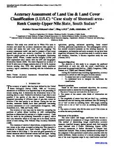
The objective of this work is to build a system that generates thematic maps from RapidEye images. Mexico is divided in around 4000 RapidEye tiles. At the moment, we have images from 2011 to 2014. This adds up to approximately 9TB of data, but the CONABIO will continue receiving images probably until 2020. Labeled data was generated by INEGI (National Institute of Statistics and Geography). The dataset consists of 238 labeled images, each 200 × 200. These tiles are just pieces of complete RapidEye images. These images were labeled manually. First, the images were segmented using Berkeley Image Segmentation algorithm (Berkeley Environmental Technology International LLC 2014). Then, the analysts received the segmented images and labeled every object for which they felt confident of the class. The classification was made according to a hierarchical scheme with three levels, developed by INEGI. The first level consists of 7 classes: Forest, Grassland, Wetland, Agricultural Land, Water, Human Settlements, and Others. ‘Others’ is particular because it contains many subclasses like clouds, roads, no vegetation, among others. The other classification levels contain 14 classes and 31 classes, respectively. Our current attempts are with the coarser level of seven classes.
Our 238 images dataset was divided in training and testing datasets, using a 70/30 ratio, performing 5-fold crossvalidation. We are evaluating the method on the first level of the classification hierarchy. The classes are Forest, Grassland, Wetland, Agricultural Land, Water, Human Settlements, and Others. We report results using a Random Forests method to classify. On our tests, Forests and Human Settlements are getting acceptable precision and recall rates. Grassland classification is performing poorly. In particular, most of the Grassland pixels are predicted as Forest. Our dataset does not have enough Water and Wetland points; so we are not concerned by those results. The confusion matrix is presented in Table 1. The horizontal axis is the predicted label; and the vertical, the true label. F G W AL Wa HS O
F
G
W
AL
Wa
HS
O
991,525 107,768 4 79,080 907 5,776 5,402
68,817 67,642 724 75,114 833 18,357 8,860
628 40 0 58 0 29 121
79,345 61,029 55 412,100 445 11,427 7,459
648 2 0 104 48 248 40
37,468 21,524 1,218 14,467 189 234,726 30,022
2,204 1,524 60 1,164 189 22,640 32,939
Table 1: Confusion matrix for the Random Forests classifier. F=Forest, G=Grassland, W=Wetland, AL=Agricultural Land, Wa=Water, HS=Human Settlements, O=Others.
Methodology
As one can see, we obtain the best performances for Forest, Agricultural Land and Human Settlements classes with precisions of 83.3%, 72.1%, 69.1%; and recalls of 84.0%, 70.8%, 80.0%, respectively.
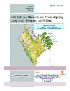
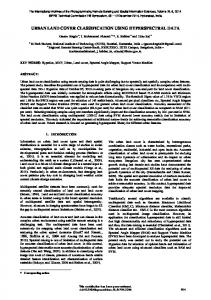
As we mentioned before, our approach is to classify textures. Our hypothesis is that each class can be characterized from the probability density distribution of the spectral bands. The methodology is divided in feature extraction and classification. Currently, we are mostly working on the feature extraction phase. For feature extraction, we segment the image to create homogeneous groups of pixels, which we expect will belong to the same class. To create these segments (or superpixels), we test Simple Linear Iterative Clustering (SLIC) (Achanta et al. 2012), and Berkeley Image Segmentation. SLIC algorithm implementation is faster than Berkeley’s, and the results were very similar for our purposes, even though Berkeley Image Segmentation supports multi-spectral images. Since RapidEye images consist of 5 bands, and the SLIC implementation is designed for grey-level and RGB images only, we applied Principal Component Analysis (PCA) to reduce dimensionality and keep most of the information in the first three components. For each segment, the system computes the density histogram of every band b and the feature vector of the segment is the vector of bins densities. So our feature space lays on X ∈ R5×k , where k is the number of bins. The limits of the histogram are computed by a previous stage where the low percentile, qlb , and the high percentile, qhb , are found. These two are calculated per band.
Work in progress At the moment, our main focus is on feature extraction. We are evaluating the possibilities of our current model and possible extensions to it. If we think of how a person could decide on which class to assign to an area, we can notice that one uses more than just color; shapes and symmetries in the texture patterns are also references to select a class. We believe that modeling those visual queues can help to improve the encoding of the class properties. For instance, a histogram of gradients and their orientations inside a segment can describe other features of the texture, which may be beneficial to distinguish between those objects that are similar chromatically but have different spatial patterns, like agriculture and grassland. Another line of work is feature learning, using techniques like Denoising Autoencoders (Vincent et al. 2008) and Triangle K-means (Coates, Ng, and Lee 2011), which have been successful in many computer vision tasks, but, to the authors knowledge, they have not been applied in LUCC projects. Given that our ground truth data covers a very small fraction of the Mexican territory, we need to find other sources
108
of labeled data, like road maps, forest inventory maps, labels from Landsat data. Each of these sources may have particular challenges. Scaling, for instance, is an important one that will be present in most of these potential ground truth new datasets.
Conclusions Although this work has been focused on RapidEye images, we are looking for a methodology that is not tied to the specifics of this sensor. We are still researching for ways to model in-class pixel dependencies. Finally, this work will be the basis for a land cover and land use change classification system.
References Achanta, R.; Shaji, A.; Smith, K.; Lucchi, A.; Fua, P.; and Susstrunk, S. 2012. SLIC superpixels compared to state-of-theart superpixel methods. IEEE Transactions on Pattern Analysis and Machine Intelligence 34(11):2274–2282. Berkeley Environmental Technology International LLC. 2014. Berkeley Image Segmentation. Available online: http://www.imageseg.com/ (accessed on 2014-10-14). Coates, A.; Ng, A. Y.; and Lee, H. 2011. An analysis of singlelayer networks in unsupervised feature learning. In International Conference on Artificial Intelligence and Statistics, 215– 223. Hansen, M.; Potapov, P.; Moore, R.; Hancher, M.; Turubanova, S.; Tyukavina, A.; Thau, D.; Stehman, S.; Goetz, S.; Loveland, T.; et al. 2013. High-resolution global maps of 21st-century forest cover change. Science 342(6160):850–853. Vincent, P.; Larochelle, H.; Bengio, Y.; and Manzagol, P.-A. 2008. Extracting and composing robust features with denoising autoencoders. In Proceedings of the 25th international conference on Machine learning, 1096–1103. ACM.
109