To be able to explore the utility of laugh- ter segments for speaker recognition, however, we first need to build a robust system to detect laughter, which is the ...
Automatic Laughter Detection Using Neural Networks Mary Tai Knox1,2 , Nikki Mirghafori1 1
2
International Computer Science Institute, Berkeley, California Department of Electrical Engineering, University of California, Berkeley {knoxm,nikki}@icsi.berkeley.edu
Abstract Laughter recognition is an underexplored area of research. Our goal in this work was to develop an accurate and efficient method to recognize laughter segments, ultimately for the purpose of speaker recognition. Previous work has classified presegmented data as to the presence of laughter using SVMs, GMMs, and HMMs. In this work, we have extended the stateof-the-art in laughter recognition by eliminating the need to presegment the data, while attaining high precision, as well as yielding higher resolution for labeling start and end times. In our experiments, we found neural networks to be a particularly good fit for this problem and the score level combination of the MFCC, AC PEAK, and F0 features to be optimal. We achieved an equal error rate (EER) of 7.9% for laughter recognition, thereby establishing the first results for nonpresegmented frame-by-frame laughter recognition on the ICSI Meetings database. Index Terms: laughter recognition, neural networks, speech in meetings.
1. Introduction Audio communication contains a wealth of information in addition to spoken words. Specifically, laughter provides cues regarding the emotional state of the speaker [1], topic changes in the conversation [2], and the speaker’s identity. Accurate laughter detection could be useful in a variety of applications. A laughter detector incorporated with a digital camera could be used to identify an opportune time to take a picture [3]. Laughter could be useful in a video search of humorous clips [4]. In speech recognition, identifying laughter could decrease word error rate by identifying nonspeech sounds [2]. The overall goal of our study is to use laughter for speaker recognition, as our intuition is that many individuals have their own distinct laugh. To be able to explore the utility of laughter segments for speaker recognition, however, we first need to build a robust system to detect laughter, which is the focus of this paper. Previous work has studied the acoustics of laughter [5, 6, 7]. Many agree that laughter has a “breathy” consonant-vowel structure [5, 8]. Some have made generalizations about laughter, such as Provine, who concluded that laughter is usually a series of short syllables repeated approximately every 210 ms [7]. Yet, others have found laughter to be highly variable [8] and thus difficult to stereotype [6]. These conclusions lead us to believe that automatic laughter detection is not a simple task. The most relevant previous work on automatic laughter detection has been that of Kennedy and Ellis [2] and Truong and van Leeuwen [1]. However, the experimental setups and objec-
tives of their work were different from ours and each other, as described below. Kennedy and Ellis [2] studied the detection of overlapped (multiple speaker) laughter in the Meetings domain. They split the data into non-overlapping one second segments, which were then classified based on whether or not multiple speakers laughed. They used support vector machines (SVMs) trained on four features: MFCCs, delta MFCCs, modulation spectrum, and spatial cues. They achieved a true positive rate of 87%. Truong and van Leeuwen [1] classified presegmented ICSI Meetings data as laughter or speech. The segments were determined prior to training and testing their system and had variable time durations. The average duration of laughter and speech segments were 2.21 and 2.02 seconds, respectively. They used Gaussian mixture models trained with perceptual linear prediction (PLP) features, pitch and energy, pitch and voicing, and modulation spectrum. They built models for each of the feature sets. The model trained with PLP features performed the best at 13.4% EER for a data set similar to the one used in our study. The goal of this work is to automatically detect segments of laughter without presegmenting the audio first. We initially experimented with SVMs, similar to the work done by Kennedy and Ellis [2]. To train the SVM, we needed to calculate and store feature statistics (mean and standard deviation) over a segment, and hence, first had to decide on a segment length. We also had to determine how often we calculated these statistics, or the offset. The offset determined the shortest duration that was classified as (non-)laughter and thus defined the precision of the start and end times. Small offsets allowed for more precise detection of laughter; however, more data storage was needed to store the statistical features for smaller offsets. We initially chose an offset of 0.5 seconds. We calculated the statistics of MFCC features over a 1 second segment like Kennedy and Ellis [2]. This approach had good results (9% EER) but did not precisely detect start and end times of laughter segments since the data was rounded to the nearest half of a second. We then decreased the offset to 0.25 seconds. This system performed better than the first with an EER of 8%. However, the time to compute the features and train the SVM increased significantly and the storage space needed to store the features approximately doubled. Furthermore, the resolution of detecting laughter was still poor (only accurate to 0.25 seconds). We also computed the EER for an offset of 0.25 seconds and a segment length of 0.5 seconds to be 13%. This suggests that the duration over which the statistics are calculated influences the accuracy of the system. The shortcomings of the SVM system (namely, the need to parse the data into segments, calculate and store to disk the statistics of the raw features, and poor resolution of start and end times) were resolved by using a neural network, which is the main technique we discuss at length in this paper. A neural
of relying on the transcripts. As a note, unlike Truong and van Leeuwen we included audio that contained non-lexical vocalized sounds other than laughter. Figure 1 shows the histogram of the laughter durations. The average laugh duration was 1.615 seconds with a standard deviation of 1.241 seconds.
3. System description 3.1. Features 3.1.1. Mel Frequency Cepstral Coefficients (MFCCs)
Figure 1: Histogram of laugh duration for the Bmr subset of the ICSI Meeting Recorder Corpus.
network was trained with features from a context window of input frames, thereby obviating the need to compute and store the mean and standard deviations since the raw data for each frame was included as a feature. The neural network was used to evaluate the data on a frame-by-frame basis thus eliminating the need to presegment the data, while at the same time achieving a good resolution to detect laughter. We experimented with MFCC and pitch features, the choice of which was inspired by previous acoustic studies in laughter characterization and automatic laughter detection. The outline for the paper is as follows: in Section 2 we describe the data used in this study, in Section 3 we describe our system set up, in Sections 4 and 5 we provide and discuss our results, and in Section 6 we provide our conclusions and ideas for future work.
2. Data We trained and tested the segmenter on the ICSI Meeting Recorder Corpus [9], a hand transcribed corpus of multi-party meeting recordings, in which each of the speakers was recorded on a close-talking microphone (which is the data used in this study) as well as distant microphones. The full text was transcribed in addition to non-lexical events (including coughs, lip smacks, mic noise, and most importantly, laughter). There were a total of 75 meetings in this corpus. In order to compare our results to the work done by Kennedy and Ellis [2] and Truong and van Leeuwen [1], we used the same training and testing sets, which were from the Bmr subset of the corpus. This subset contains 29 meetings. The first 26 were used for training and the last 3 were used to test the detector. We trained and tested only on data which was hand transcribed to be either laughter or non-laughter. Laughter-colored speech, that is, cases in which the hand transcribed documentation had both speech and laughter listed under a single start and end time were disregarded since we would not specifically know which time interval(s) contained laughter. Also, if the transcription did not include information for a period of time for a channel, that audio was excluded. This exclusion reduced training and testing on cross-talk and allowed us to train and test on channels only when they were in use. Ideally, an automatic silence detector would be employed in this step instead
In this study, MFCCs were used to capture the spectral features of (non-)laughter. The first order regression coefficients of the MFCCs (delta MFCCs) and the second order regression coefficients (delta-delta MFCCs) were also computed and used as features for the neural network. We used the first 12 MFCCs as well as the 0th coefficient, which were computed over a 25 ms window with a 10 ms forward shift, as features for the neural network. MFCC features were extracted using the Hidden Markov Model Toolkit (HTK) [10]. 3.1.2. Pitch and energy Studies in the acoustics of laughter [5, 6] and in automatic laughter detection [1] investigated the pitch and energy of laughter as potentially important features. Similarly, we used the ESPS pitch tracker get f0 [11] to extract the fundamental frequency (F0 ), local root mean squared energy (RMS), and the highest normalized cross correlation value found to determine F0 (AC PEAK) for each frame. The delta and delta-delta coefficients were computed for each of these features as well. 3.2. Neural network We did frame-wise laughter detection. Since the frames were short in duration (10 ms) and each laughter segment was on average 1.615 seconds in this data set, we decided it would be best to use a context window of features as inputs in the neural network. A neural network with one hidden layer was trained using QuickNet [12]. The input to the neural network was a window of feature frames, where the center frame was the target frame. We used the softmax activation function to compute the probability that the frame was laughter. To prevent over-fitting, the data used to train the neural network was split into two groups: training (the first 21 Bmr meetings) and cross validation (the last 5 meetings from the original training set). The neural network weights were updated based on the training data via the back-propagation algorithm and then the cross validation data was scored after every training epoch resulting in the cross validation frame accuracy (CVFA). Training was concluded once the CVFA increased by less than 0.5% for a second time.
4. Experiments and results 4.1. Parameter settings We first needed to determine the context window size and the number of hidden units in the neural network. In Section 1, we showed that the EERs of the SVM systems were dependent on the segment length. Likewise, the neural network results were dependent on the size of the input window size, or context window. Empirically, we found that a window of 75 consecutive frames (0.75 seconds) worked well. To make the classification
t
w
i
n
d
o
w
w
h
7
5
f
r
a
m
e
s
(
7
5
0
m
s
)
i
Table 1: EERs (%) of individual systems. 1
0
1
3
5
3
6
3
7
� �
� 3
3
6
�
3
5
7
.
.
.
.
.
.
t
t
a
r
g
e
t
f
r
a
m
e
(
1
0
m
s
)
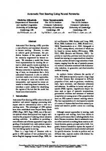
Figure 2: For each frame evaluated, features from a context window of 75 frames were inputted to the neural network.
of laughter based on the middle frame, we set the offset to 37 frames. In other words, the inputs to the neural network were the features from the frame to be classified and the 37 frames before and after this frame. Figure 2 shows our windowing technique. We also had to determine the number of hidden units. MFCCs were the most valuable features for Kennedy and Ellis [2] and we suspected we would observe similar results. Thus, we used the MFCCs as the input features and modified the number of hidden units while keeping all other parameters the same. Based on the accuracy on the cross validation set, we saw that 200 hidden units performed best. Similarly, we varied the number of hidden units using F0 features. The CVFA was approximately the same for a range of hidden units but the system with 200 was marginally better than the rest. 4.2. Systems The neural networks were first separately trained on the four classes of features: MFCCs, F0 , RMS, and AC PEAK. The EERs for each of the classes is shown in Table 1. Each column lists the EER for a neural network trained with the feature itself, the deltas, the delta-deltas, and the feature level combination of the feature, delta, and delta-delta (the “All” System). We combined the “All” systems on the score level to improve our results using another neural network, this time using a smaller window size. Since each of the inputs was the probability of laughter for each frame, we shortened the input window size of the combiner neural network from 75 frames to 9 and kept the number of hidden units at 200. Since the system using MFCC features had the lowest EER, we combined MFCCs with each of the other classes of features. Table 2 shows that after combining, the MFCC+AC PEAK system performed the best. We then combined the MFCC+AC PEAK system with the RMS system and the F0 system. Finally, we combined all of the systems and computed the EER. We also computed score level combinations of the delta MFCC system with the “All” systems of the other classes of features, thereby combining the best system for each class of features. These results were all better than the previous score level combinations as shown in Table 3. Since the score level combinations had at most 4 features (1 per system), we decided to run the combiner with fewer hidden units (2) as well. The results are shown in Table 3.
5. Discussion From Table 1, it is clear that MFCC features outperformed all of the pitch related features. This is consistent with Kennedy and Ellis’ [2] results. For Truong and van Leeuwen [1], PLP features outperformed the other features. PLPs, like MFCCs, have
Feature ∆ ∆∆ All
MFCCs 11.35 9.62 11.23 10.66
F0 23.26 24.42 27.83 22.80
RMS 32.22 26.52 26.62 26.01
AC PEAK 16.75 22.37 27.61 16.72
Table 2: EERs (%) of score level combinations of “All” systems with 200 hidden units. MFCC+F0 MFCC+RMS MFCC+AC PEAK MFCC+AC PEAK+RMS MFCC+AC PEAK+F0 MFCC+AC PEAK+RMS+F0
EER 9.38 8.59 8.15 8.19 8.61 8.80
perceptually scaled frequency content so it is not surprising that they performed well for the task of laughter detection, also. AC PEAK features had the second lowest EERs, which suggests that the largest cross correlation of an audio signal helps in detecting laughter. This seems reasonable since laughter is repetitive [7]. However, Provine found that the repetitions were every 210 ms, which exceeds the time used to compute the cross correlation in this study, since we focused on low level framewise features. In general, the “All” systems scored the best with the exception of the MFCCs. MFCCs scored best using the delta features alone. This could be a result of not increasing the number of hidden units despite increasing the input features by a factor of three for a total of 39 features (as opposed to 13) for each of the 75 frames. We also computed the EERs for the F0 , RMS, and AC PEAK systems using 50 hidden units. We thought that since they had fewer features than the MFCCs, fewer hidden units would be needed to accurately determine the weights for the features. Our results were inconclusive. Three of the twelve systems improved (had a smaller EER) while the other systems performed worse. Comparing the score level combinations, using the delta MFCC system was better than using the “All” MFCC system. This seems reasonable since the delta MFCC system outperformed the “All” MFCC system. Also, decreasing the number of hidden units in the score level combination from 200 to 2 made all of the results marginally worse. We also decreased the hidden units to 2 for the score level combinations of the “All” systems shown in Table 2. In that case, two of the results improved and the other four worsened. Although the EERs changed when the number of hidden units was modified from 200 to 2, they were all within 0.42% of each other. The score level combination of the delta MFCC, “All” AC PEAK, and “All” F0 systems performed the best at 7.91%. The addition of the “All” RMS system caused the EER to slightly increase. The reason may be that the “All” RMS system was worse than the other systems, thereby adding noise to the combination. Also, the RMS feature is similar in content to the 0th MFCC, so it is not surprising that adding a noisy system with redundant information did not improve the results. Directly comparing our results to previous work was a prob-
Table 3: EERs (%) of score level combinations of the delta MFCC system with other “All” systems for 200 and 2 hidden units. Number of hidden units ∆MFCC+F0 ∆MFCC+RMS ∆MFCC+AC PEAK ∆MFCC+AC PEAK+RMS ∆MFCC+AC PEAK+F0 ∆MFCC+AC PEAK+RMS+F0
200 8.17 8.08 7.92 7.92 7.91 8.01
2 8.34 8.26 7.96 8.01 7.99 8.12
lematic task for two reasons: scored data segments were not identical and segment weights were different. Truong and van Leeuwen trained and tested their systems using two datasets from the Bmr subset of the Meetings Corpus. The first dataset was similar to ours, in that the data was labeled as (non)laughter based on the transcriptions. Differences in the first dataset were that non-lexical vocalized sounds other than laughter were not part of their dataset but were part of ours. Their second dataset further differed from ours as transcribed laughter segments that were inaudible or found to include speech were verified through listening and excluded. The second reason for the lack of direct comparison is that Truong and van Leeuwen’s goal was to classify presegmented data so all of the scoring was done on the segment level, where segments varied in duration. Since our goal was to segment laughter, our scoring was performed on the frame level, with equal weights for all frames. Our best system had an EER of 7.91% while previous work performed by Truong and van Leeuwen achieved an EER of 13.4% and 7.1% on the first and second datasets, respectively [1].
6. Conclusion and future work In conclusion, we have extended previous work on laughter detection by eliminating the need for presegmented data. We have found neural networks to be a good match to automatically detect frames containing laughter, as no extra off-line computation and disk storage is needed to compute average statistic features over a segment (as for SVMs), while yielding a higher detection precision of start and end times (up to 10 ms for our study). Using features from a context window, we were able to determine if a single frame contained laughter with an EER of 7.91% for our best system, which was the score level combination of the delta MFCC, “All” AC PEAK, and “All” F0 systems. Although our study was run on the same database as previous work, our results were not directly comparable for reasons cited in Section 5. We hope that our work serves as a baseline for future work on frame-by-frame laughter recognition on the Meetings database, which provides an excellent testbed for laughter research. We plan on computing the feature level combinations and are currently exploring the use of additional features to detect laughter. Trouvain noted the repetition of a consonant-vowel syllable structure [8]. We have run a phoneme recognizer on the audio and are using neural networks to detect patterns of phoneme repetition. Another approach is to compute prosodic features, including pitch and energy, over longer intervals of time. Since laughter repeats every 210 ms (or 4.76 Hz) [7], prosodic features may capture this repetitiveness. By adding more features to our system, we hope to further improve our results in order to more thoroughly investigate the speaker discriminative power of laughter.
7. Acknowledgments The authors would like to thank Khiet Truong and Lyndon Kennedy for generously discussing their work and sharing their data. The material in this paper is based upon work partially supported by the NSF under grant No. 0329258.
8. References [1]
Truong, K.P. and Van Leeuwen, D.A., “Automatic detection of laughter”, In Proceedings of Interspeech, Lisbon, Portugal, 2005.
[2]
Kennedy, L. and Ellis, D., “Laughter detection in meetings”, NIST ICASSP 2004 Meeting Recognition Workshop, Montreal, 2004.
[3]
Carter, A., “Automatic acoustic laughter detection”, Masters Thesis, Keele University, 2000.
[4]
Cai, R., Lu, L., Zhange, H.-J., Cai, L.-H., “Highlight sound effects detection in audio stream”, in Proc. Intern. Confer. on Multimedia and Expo, Baltimore, MD, 2003.
[5]
Bickley, C., Hannicutt, S., “Acoustic analysis of laughter”, In Proc. ICSLP, pp. 927–930, Banff, Canada, 1992.
[6]
Bachorowski, J., Smoski, M., Owren, M., “The acoustic features of human laughter”, Acoustical Society of America, pp. 1581–1597, 2001.
[7]
Provine, R., “Laughter”, American Scientist, January– February 1996.
[8]
Trouvain, J., “Segmenting phonetic units in laughter”, In Proc ICPhS, Barcelona, 2003.
[9]
Janin, A., Baron, D., Edwards, J., Ellis, D., Gelbart, D., Morgan, N., Peskin, B., Pfau, T., Shriberg, E., Stolcke, A., Wooters, C., “The ICSI meeting corpus”, ICASSP, Hong Kong, 2003.
[10] Hidden Markov Model http://htk.eng.cam.ac.uk/.
Toolkit
(HTK):
[11] ESPS version 5.0 programs manual,Washington, DC, 1993. [12] QuickNet: http://www.icsi.berkeley.edu/Speech/qn.html.